| Issue |
A&A
Volume 703, November 2025
|
|
|---|---|---|
| Article Number | A266 | |
| Number of page(s) | 11 | |
| Section | Planets, planetary systems, and small bodies | |
| DOI | https://doi.org/10.1051/0004-6361/202555889 | |
| Published online | 24 November 2025 | |
The resilience of the sailboat stable region
1
LIRA, Observatoire de Paris, Université PSL, Sorbonne Université, Université Paris Cité, CY Cergy Paris Université, CNRS,
92190
Meudon,
France
2
São Paulo State University (UNESP), School of Engineering and Sciences,
Guaratinguetá,
SP
12516-410,
Brazil
3
Eberhard Karls Universität Tübingen,
Auf der Morgenstelle, 10,
72076
Tübingen,
Germany
4
Observatório Nacional (ON)/MCTI,
Rio de Janeiro,
RJ
20921-400,
Brazil
★ Corresponding author: This email address is being protected from spambots. You need JavaScript enabled to view it.
Received:
10
June
2025
Accepted:
2
October
2025
Abstract
Context. Binary systems host complex orbital dynamics where test particles can occupy stable regions, despite strong gravitational perturbations. The sailboat region, discovered in the Pluto–Charon system, hosts highly eccentric S-type orbits at intermediate distances between the two massive bodies. This region challenges traditional stability concepts by supporting eccentricities up to 0.9 in a zone typically dominated by chaotic motion.
Aims. We investigate the sailboat region’s existence and extent across different binary system configurations. We examine how variations in mass ratio, secondary body eccentricity, particle inclination, and argument of pericenter affect this stable region.
Methods. We performed 1.2 million numerical simulations of the elliptic three-body problem to generate four datasets exploring different parameter spaces. We trained XGBoost machine learning models to classify stability across approximately 109 initial conditions. We validated our results using Poincaré surface of section and Lyapunov exponent analysis to confirm the dynamical mechanisms underlying the stability.
Results. The sailboat region exists only for binary mass ratios of μ = [0.05, 0.22]. Secondary body eccentricity severely constrains the region, following an exponential decay of es,max ≈ 0.016 + 0.614exp(−25.6μ). The region tolerates particle inclinations up to 90° and persists in retrograde configurations for μ ≤ 0.16. Stability requires a specific argument of pericenter within ±10° to ±30° of ω = 0° and 180°. Our machine learning models have achieved over 97% accuracy in predicting stability.
Conclusions. The sailboat region shows strong sensitivity to system parameters, particularly secondary body eccentricity. Among Solar System dwarf planet binaries, we find that Pluto–Charon, Orcus–Vanth and Varda–Ilmarë systems could harbor such regions. The combination of numerical simulations and machine learning provides an efficient approach for mapping stability in complex gravitational systems.
Key words: methods: numerical / celestial mechanics / minor planets, asteroids: general
© The Authors 2025
 Open Access article, published by EDP Sciences, under the terms of the Creative Commons Attribution License (https://creativecommons.org/licenses/by/4.0), which permits unrestricted use, distribution, and reproduction in any medium, provided the original work is properly cited.
This article is published in open access under the Subscribe to Open model. This email address is being protected from spambots. You need JavaScript enabled to view it. to support open access publication.
1 Introduction
Binary systems, where two massive bodies orbit their common center of mass, represent fundamental configurations in celestial mechanics. Understanding the dynamics of test particles within these systems has direct applications for planetary formation, spacecraft mission design, satellite detection, and the study of natural debris distributions.
Among the various orbital configurations possible in binary systems the S-type orbits, where particles orbit one of the massive bodies, exhibit complex stability patterns. These patterns depend on multiple parameters including mass ratio, eccentricity, and orbital inclination.
The Pluto–Charon system provides an exceptional natural laboratory for studying binary dynamics. With a mass ratio of μ ~ 0.12 and a separation distance of d = 19 595 km (Brozović & Jacobson 2024), this system challenges traditional models due to Charon’s significant mass relative to Pluto. The system also hosts four small satellites (Styx, Nix, Kerberos, and Hydra) in P-type orbits around the system’s barycenter, demonstrating the richness of its dynamical environment.
Previous investigations of the Pluto–Charon system revealed unexpected stable regions for test particles. Winter et al. (2010); Giuliatti Winter et al. (2013, 2014) made extensive numerical simulations to map S-type orbital stability around both Pluto and Charon. Their works identified three distinct stable regions for prograde particles: the first around Charon extending to 0.2d with eccentricities below 0.6, the second region lies close to Pluto and extends to 0.5d, while the third region, named the “sailboat region” due to its distinctive shape in the (a, e) parameter space, occupies the mid-distance between Pluto and Charon with high eccentricities ranging from 0.2 to 0.9.
Unlike typical stable regions that favor near-circular orbits or occupy mean-motion resonances, this region allows for highly eccentric orbits at intermediate distances. Giuliatti Winter et al. (2014) demonstrated through Poincaré surfaces of section that the sailboat region corresponds to a family of periodic orbits (family “BD”) derived from the circular restricted three-body problem (Broucke 1968). Further analysis showed that the region persists for inclinations up to 90° and exists within specific intervals of the argument of pericenter, namely: ω = [−10°, 10°] and [160°, 200°], reaching maximum extent at ω = 0° and 180°.
This work investigates the resilience of the sailboat region by exploring how it responds to variations in key system parameters. We examine the effects of changing the binary mass ratio, secondary body eccentricity, particle inclination, and argument of pericenter on the existence and extent of this stable region. To map the vast parameter space efficiently, we combine direct numerical simulations with machine learning algorithms; thus, our work is focused on numerically mapping the sailboat region’s extent across multiple parameter spaces rather than pursuing analytical solutions, which remain challenging for such complex multi-parameter dynamical systems. A similar study was applied by Pinheiro et al. (2025), who performed machine learning techniques to map the stability of a star-planet-particle test system, achieving an accuracy of 98.48%. We first generate training datasets through targeted three-body simulations, then applied a supervised learning to predict stability across billions of initial conditions that would be computationally prohibitive to simulate directly.
The paper is organized as follows. Section 2 examines different types of binary systems and their characteristics. Section 3 describes our numerical simulation methods and machine learning approach. Section 4 analyzes how the sailboat region varies with binary mass ratio. Section 5 investigates the effects of secondary body eccentricity, particle inclination, and argument of pericenter. Section 6 validates our results using stability verification methods, including a Poincaré surface of section and Lyapunov exponent analysis. The last section presents our concluding remarks.
2 Binary systems
To understand the broader context of sailboat regions beyond the Pluto–Charon system, we chose to examine binary configurations across different astrophysical environments. This analysis helps identify which types of binary systems could potentially harbor sailboat regions and provides observational targets for future studies. Since the sailboat region requires specific mass ratio ranges and orbital configurations, understanding the distribution of binary system properties is important for predicting where such regions might exist.
Binary star systems can be classified into three distinct types based on the separation distance between the components and their physical sizes. Detached systems have both stars well within their Roche lobes, maintaining stable orbital configurations without mass exchange. Semi-detached systems have one star that has filled its Roche lobe, enabling mass transfer to its companion and creating dynamically active environments. Contact systems have both stars filling their Roche lobes, resulting in continuous mass exchange between the components (Kopal 1955).
Figure 1 presents the distribution of semimajor axis (as) in units of the primary star radius (rstar) versus binary mass ratio (μ) for 489 eclipsing binary systems from observational surveys. The sample has 100 contact systems, 232 semidetached systems, and 157 detached systems, compiled from three catalogs: the catalog of DMS-type eclipsing binaries (Svechnikov & Perevozkina 2004), catalog of early-type contact binaries (Bondarenko & Perevozkina 2004), and semidetached eclipsing binaries (Surkova & Svechnikov 2004).
The majority of binary systems with mass ratios comparable to that of Pluto–Charon (indicated in black) are semidetached configurations, as shown in Figure 1. The ongoing mass transfer processes in these systems create unstable dynamical environments in the circumbinary region. However, four detached systems exhibit μ < 0.25 with separation distances ranging from 2 to 8 rstar. These detached configurations provide stable dynamical environments that can harbor sailboat regions, consistent with the findings of Giuliatti Winter et al. (2014). Similar stability considerations apply to smaller binary systems within our Solar System, particularly among trans-Neptunian dwarf planet binaries.
The term “dwarf planet” was introduced during the XXVIth General Assembly of the IAU. Unlike planets, this new category of objects has not cleared the surrounding region of their orbits. Table 1 shows the ten largest confirmed or candidate dwarf planets that host at least one satellite. This table includes the mass ratio of the system, orbital semimajor axis (as), and eccentricity (es) of each satellite.
All these bodies are trans-Neptunian objects (TNOs). Among the confirmed dwarf planets, only Ceres and Sedna have no discovered satellites, while Pluto hosts five satellites, and Haumea hosts two: Hi’iaka and Namaka.
Moreover, Quaoar and Haumea have ring systems that orbit close to the 1:3 spin–orbit resonance with their primary body. In the case of Quaoar, its two rings are located outside its Roche limit (Pereira et al. 2023; Morgado et al. 2023; Ortiz et al. 2017).
The Pluto–Charon system is the only trans-Neptunian dwarf planet that has been visited by a spacecraft. Two systems, Orcus–Vanth and Varda–Ilmarë, have μ values close to that of Pluto–Charon, with μ = 0.16 and 0.083, respectively. This suggests that both binaries likely exhibit a sailboat region similar to the Pluto system. Investigating stability regions around these bodies can be helpful for future space missions and observation campaigns to identify the most probable locations for discovering new objects or ring systems.
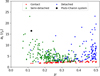 |
Fig. 1 Diagram of a binary star system (d × μ), where d represents the separation distance between the stars and μ is the binary mass ratio. The diagram categorizes the binary types as follows: blue for detached, green for semidetached, and red for contact. The black point corresponds to the Pluto–Charon system. |
Binary systems of dwarf planet and their satellites in our Solar System.
3 Methods
Having identified potential binary systems that have the capacity to harbor sailboat regions, we go on to examine the computational methods used to map their stability. To investigate the stability of the sailboat region across different binary system configurations and orbital parameters, we implemented two complementary approaches. First, we performed direct numerical simulations of the three-body problem, as described in Sect. 3.1. These simulations generated both stability maps and training data for our machine learning models. Then, we applied supervised learning algorithms to classify stability across a broader parameter space, as detailed in Sect. 3.2. This combined methodology allowed us to efficiently explore stability conditions that would be computationally prohibitive through direct simulations alone.
3.1 Numerical method
To characterize the sailboat region across different parameter spaces, we performed extensive numerical simulations of the elliptic three-body problem. We modeled a dimensionless binary system with test particles in S-type orbits around the primary body, subject to gravitational perturbations from the secondary body.
In our simulations, we defined the primary body as a point mass with Mp = 1 − μ, where μ represents the binary mass ratio. The secondary body has a mass of ms = μ, a semimajor axis of as = 1, and collision radius (rs) defined as
![Mathematical equation: $\[r_s=0.1\left[\left(1-e_{\mathrm{s}}\right) \sqrt[3]{\frac{\mu}{3}}\right],\]$](/articles/aa/full_html/2025/11/aa55889-25/aa55889-25-eq1.png) (1)
(1)
where es is the secondary body’s eccentricity, initially set to zero but varied in later simulations as described in Sect. 5.1. This collision radius formulation accounts for the Hill sphere of the secondary body, scaled by a factor of 0.1 to represent the effective collision cross-section. The (1 − es) term adjusts for orbital eccentricity, ensuring that the collision radius remains appropriate for eccentric secondary orbits. The ![Mathematical equation: $\[\sqrt[3]{\mu / 3}\]$](/articles/aa/full_html/2025/11/aa55889-25/aa55889-25-eq2.png) factor represents the Hill radius normalization in the three-body problem. This formulation ensures that particles approaching within the secondary’s gravitational sphere of influence are considered collided, preventing artificial close encounters.
factor represents the Hill radius normalization in the three-body problem. This formulation ensures that particles approaching within the secondary’s gravitational sphere of influence are considered collided, preventing artificial close encounters.
We initially simulated 300 000 binary systems, randomly selecting the mass ratio μ from a uniform distribution in the range [0.01–0.3]. For test particles in these systems, we also randomly selected orbital parameters from uniform distributions: semimajor axis a = [0.45–0.7] and eccentricity e = [0–0.99]. All other orbital elements of both the secondary body and test particles were set to zero. Using the REBOUND package with the IAS15 integrator (Rein & Spiegel 2015), we integrated each system for 104 × 2π time units, following Winter & Vieira Neto (2001), who demonstrated this duration is sufficient to establish orbital stability.
Simulations terminated when particles either collided with the secondary body or were ejected from the system (defined as e ≥ 1 or a > 1). For each initial condition, we recorded the outcome (stable or unstable) and the termination cause (when applicable). This complete dataset, containing both stable and unstable particles with their respective parameters, comprised the training data for our machine learning algorithms.
To explore additional parameter dependencies, we generated three more datasets of 300 000 simulations each, systematically varying the secondary body eccentricity (es), particle inclination (i), and argument of pericenter (ω). Table 2 summarizes these datasets and their objectives.
For each dataset, we optimized the machine learning models through cross-validation, class imbalance correction, and parameter tuning. The resulting models allowed us to predict stability for more than 3.6 billion initial conditions, far beyond what would be computationally feasible through direct simulation.
Description of dataset parameters.
3.2 Machine learning approach
We employed the eXtreme Gradient Boosting (XGBoost) algorithm to classify the orbital stability. This supervised learning method performs binary classification, categorizing particles as either stable or unstable based on their orbital parameters. The effectiveness of this algorithm in classifying stable orbits has been demonstrated in previous studies, such as Tamayo et al. (2016) and Pinheiro et al. (2025).
XGBoost builds an ensemble of decision trees through sequential training, where each new tree corrects errors from previous iterations (Géron 2022). The algorithm computes residuals for the predictions and refines the model through successive iterations (Wade & Glynn 2020), making it particularly effective for our classification task.
We divided our data set into training and validation (80% of the data) and test (20%) sets. The training data established predictive patterns, the validation data optimized the model parameters, and the test data provided an unbiased performance evaluation (Shalev-Shwartz & Ben-David 2014). We implemented k-fold cross-validation by partitioning the training data into subsets, using each subset iteratively for validation while training on the remaining data. This technique prevents overfitting and improves generalization (Hastie et al. 2009).
Model optimization involved tuning both hyperparameters and classification thresholds. We selected optimal hyperparameters through grid search (Weerts et al. 2020). For classification thresholds, we adjusted the default 0.5 probability cut-off to address class imbalance in our datasets, as the stability cases were significantly outnumbered by instability cases in certain parameter regimes.
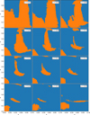 |
Fig. 2 Stability maps in the (a, e) plane for binary systems with mass ratios μ = [0.01–0.23]. Stable initial conditions are shown in orange, unstable in blue. All particles are in coplanar orbits around the primary body with ω = Ω = f = 0°. |
4 Analysis of the sailboat region for different binary mass ratios
The first dataset consisted of three freedom parameters: μ, a, and e. This stage was aimed at verifying how the sailboat region changes with varying mass ratios of the binary system.
This dataset contained 300 000 samples with the following distribution: 77.98% resulted in collisions, 0.75% in particle ejection, and 21.27% remained stable throughout the simulations. To address this imbalanced class distribution, we implemented a random oversampling technique, selecting samples from the minority class and adding them to the training dataset.
Our best model achieved 98.53% accuracy, measuring the ratio of correctly predicted outcomes. For imbalanced classification problems, we evaluated additional performance metrics: recall and precision. Recall measures the ratio of correctly identified samples within each class, reaching 97% for stable and 99% for unstable classes. Precision measures the ratio of correct classifications within each predicted class, achieving 97% for stable and 99% for unstable classes. This accuracy significantly exceeds the ~90% threshold typically considered acceptable for astronomical classification tasks.
Figure 2 presents stability maps derived from machine learning predictions for binary systems with mass ratios in the range μ = [0.01–0.23]. Each diagram represents 247 500 different initial conditions, with particle semimajor axis a = [0.45–0.7] and eccentricity e = [0–0.99] using step sizes of Δa = Δe = 0.001. Our complete analysis covered the range μ = [0.01–0.30], revealing that the sailboat region disappears entirely for μ ≥ 0.24, placing an upper limit on the mass ratio for the existence of this region.
As shown in Figure 2, binary systems with μ ≤ 0.04 have a contiguous stable region around the primary body extending up to ~0.7. In the interval a = [0.55–0.68], stable particles can reach high eccentricities, though they remain below e = 1 due to the stability criterion.
For μ = 0.05, the stability map reveals two distinct regions: (i) one confined to a < 0.52 and e ≤ 0.4 and (ii) the sailboat region located at a = [0.52–0.7]. This represents the smallest mass ratio where we can identify two separated stable regions, marking where the sailboat region gets detached from the inner stability region. As μ increases, the sailboat region progressively diminishes in size until it completely vanishes at μ = 0.22.
The minimum particle eccentricity of the sailboat region increases with higher μ values. For a binary system with μ = 0.07, sailboat particles have eccentricity e > 0.1, while for μ = 0.09 the eccentricities increase to e > 0.18. When μ = 0.10, the sailboat splits into two regions: the larger one at a = [0.52–0.67] and e = [0.2–0.8], while the smaller region contains particles with highly eccentric orbits (e > 0.85).
Some eccentric stable orbits (e > 0.85) in the sailboat region can become unstable depending on the size of the primary body. Figure 3 shows the sailboat region for a binary with μ = 0.12 (similar to the Pluto–Charon system). The red dashed line indicates when the pericenter of the particle has the same distance as Pluto’s radius. As shown in Figure 3, all particles with e > 0.9 (above the red dashed line) will collide with Pluto, which matches the results of Giuliatti Winter et al. (2014).
For binary systems with μ = 0.15, the main region in the sailboat is constrained to a range of a = [0.52–0.63] and e = [0.22–0.7], becoming less eccentric and losing its sailboat-like shape. When μ = 0.16 the maximum eccentricity for this region is ~0.6, and for μ = 0.18, it is situated at a = [0.5–0.6] with e < 0.5, showing a gradual shift towards the primary body and a decrease in the maximum eccentricity. For μ = 0.22, a new stable region emerges at a > 0.65 and e ~ 0.4. This region expands in size and merges with the remaining sailboat at μ = 0.23.
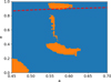 |
Fig. 3 Sailboat region for a binary system with μ = 0.12 (the closest case with Pluto–Charon system, where Charon has eccentricity). The red dashed line represents the pericenter of the particle in the same distance of Pluto’s radius. There is other stable regions in the range a = [0.45–0.7], not showed in the plot. |
5 Different initial conditions
5.1 Eccentric secondary body case
Next, we investigated how the secondary body’s eccentricity affects the sailboat region stability. This dataset contains four parameters: binary mass ratio (μ = [0.01–0.23]), particle semimajor axis (a = [0.45–0.7]), particle eccentricity (e = [0–0.99]), and secondary body eccentricity (es = [0–0.99]).
The overall outcome from 300 000 simulated samples shows that 1.77% of the particles remain stable, while 98.23% become unstable. Among the unstable particles, 95.39% are ejected and 2.84% collide with the secondary body. Our best machine learning model utilizes the adaptive synthetic (ADASYN) oversampling technique to handle this significant class imbalance, where the ratio between minority and majority classes is approximately 1:50.
The ADASYN method generates synthetic samples for the minority class in the training dataset based on the distribution of samples belonging to that class in the feature space (He et al. 2008). Our best machine learning model achieves an accuracy of 99.55%. Specifically, for the stable class, we obtain a recall and precision of 87%, and almost 100% for the unstable class. From 60 000 samples in the test dataset, the model correctly classifies 913 as stable and 58 817 as unstable, misclassifying only 270 particles (135 from the stable class classified as unstable and 135 from the unstable class classified as stable).
We employed our machine learning model to predict stability maps (a × e) for each μ ≤ 0.22 and determine the maximum secondary body eccentricity value where the sailboat region completely vanishes, using a step size of Δes = 0.001. Figure 4 shows the maximum eccentricity of the secondary body where the sailboat region exists (blue dots) for different mass ratios. The red curve represents a fit obtained through the least squares method. Each green square represents a binary system of dwarf planets and their satellites shown in Table 1, while the black square indicates the Pluto–Charon system.
Small changes in the secondary body eccentricity are sufficient to substantially decrease the extension of the sailboat region. An empirical expression for the maximum eccentricity value (es,max) as a function of μ can be expressed as
![Mathematical equation: $\[e_{s, \max } \approx(0.016 \pm 0.006)+(0.614 \pm 0.023) e^{(-25.626 \pm 1.636) \mu} .\]$](/articles/aa/full_html/2025/11/aa55889-25/aa55889-25-eq3.png) (2)
(2)
This equation indicates a strong exponential decay between es,max and the μ parameter. Figure 4 shows that all dwarf planets present in Table 1 may exhibit a sailboat region, indicating potential regions for hosting satellites or ring systems. It is even possible to design missions with spacecraft studying the system from an orbit within this region due to its stability.
Figure 5 shows the evolution of the sailboat region as the secondary body eccentricity changes for binary systems with mass ratios of μ = 0.05, 0.12, and 0.22.
Particles with lower eccentricity within the sailboat region become unstable as the eccentricity of the secondary body increases. In Figure 5, for μ = 0.05 and es = 0.2, only particles with e ~ 0.8 survive. When μ = 0.12 with es = 0.03 and μ = 0.22 with es = 0.007, only particles with e approaching unity survive, however they will probably collide with the primary body.
When disregarding particles with e > 0.9 to prevent collisions with the primary body, the maximum limit of secondary body eccentricity shows significant changes for μ ≥ 0.12 compared with the results shown in Figure 4. For μ values ranging from 0.12 to 0.16, the maximum eccentricity is 0.04. However, for μ = 0.17, es,max decreases to 0.036, a difference of 0.004 when considering that stable particles exceeding eccentricity 0.9 become unstable. For μ = 0.18 and 0.19, the value of es,max = 0.033, while for μ = 0.20 and 0.21, es,max reaches 0.018. These results demonstrate that secondary body eccentricity imposes the strongest constraint on sailboat region existence, with tolerance decreasing exponentially as μ increases.
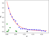 |
Fig. 4 Maximum eccentricity of secondary body (blue dots) versus mass ratio of the system. The red curve represents a fitted model obtained using the least squares method. Green squares denote binary systems of dwarf planets and their satellites, while the black square represents the Pluto–Charon system. |
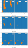 |
Fig. 5 Stability maps (a × e) showing the evolution of the sailboat region with changing secondary body eccentricity for binary systems with mass ratios of μ = 0.05, 0.12, and 0.22. |
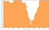 |
Fig. 6 Stability regions for different particle orbital inclinations. Orange areas indicate inclination values where stable regions exist within a = [0.4–0.7] for various μ. The gaps in coverage indicate parameter combinations where the sailboat region becomes unstable. |
5.2 Inclined particle case
To analyze how particle inclination affects the sailboat region, we generated a third dataset of 300 000 samples with four parameters: binary mass ratio (μ = [0.01–0.23]), particle semimajor axis (a = [0.45–0.7]), particle eccentricity (e = [0–0.99]), and orbital inclination (i = [0°−180°]).
This dataset shows a different class distribution compared to the eccentric secondary body case, with 20.11% stable particles and 79.89% unstable particles. Among the unstable cases, 79.75% result in ejection and only 0.14% in record collisions. The higher proportion of stable particles compared to the previous dataset reduces the class imbalance problem, although oversampling techniques remain necessary for optimal model performance.
Our best machine learning model employs a Synthetic Minority Oversampling Technique (SMOTE) approach to handle the remaining class imbalance. SMOTE creates synthetic samples within the training data by generating new instances for the minority class based on the euclidean distance between nearest neighbors, using a multiplicative factor between 0 and 1 (Chawla et al. 2002). This approach differs from ADASYN by focusing on the feature space structure rather than the local density distribution.
The optimized model achieves an accuracy of 97.15%, with precision and recall of 93% for the stable class and 98% for the unstable class. Using this model, we predict stability diagrams in the (a × e) space from i = 0° to 180°, with each step incrementing by Δi = 1°. This analysis covers each μ ≤ 0.22 with step size Δμ = 0.01. Figure 6 shows where stable regions exist within the range a = [0.45–0.7] for different values of μ and particle orbital inclination.
For the highest mass ratio, μ = 0.22, even a 2° inclination eliminates stability within a = [0.45–0.70]. At μ = 0.21, the region persists up to i ≈ 20°, disappears, then reappears at i ≈ 35° and extends to i ≈ 70°. The gap at i < 35° may indicate limited model generalization due to sparse stable particles in this parameter space. Retrograde regions appear at i ≈ 140° and reach maximum extent at i = 180°, albeit only for μ < 0.17.
For mass ratios between 0.17 and 0.20, the sailboat region survives up to i = [85°−95°]. When μ ≤ 0.16, the region remains stable for i = [90°−100°], consistent with the findings from Giuliatti Winter et al. (2013) for the Pluto–Charon system. For μ = [0.07–0.10], stability extends to i ~ 105°, with retrograde regions appearing at progressively lower inclinations as μ decreases.
For the smallest mass ratios, μ = 0.05 and 0.06, the sailboat region shows continuous existence across all inclinations, reaching minimum size at i = 110° before expanding again toward retrograde inclinations. Figure 7 illustrates the sailboat evolution for μ = 0.05 and 0.12 at representative inclinations. These results show that the strong resilience of the sailboat to inclination changes.
5.3 Varying the argument of pericenter
Our final dataset explores how the argument of pericenter affects sailboat region stability. We simulated 300 000 systems with four parameters: binary mass ratio (μ = [0.01–0.23]), particle semimajor axis (a = [0.45–0.7]), particle eccentricity (e = [0–0.99]), and argument of pericenter (ω = [0°−360°]).
The simulation outcomes show 11.5% of particles remaining stable throughout the integration period, while 87.3% experienced ejection and 1.2% collided with the secondary body. This class distribution presents a moderate imbalance compared to the eccentric secondary body case.
Our optimized machine learning model employed random oversampling to address class imbalance, achieving 98.5% accuracy. The stable class achieved 94% recall and 93% precision, while the unstable class reached 99% for both metrics, demonstrating reliable classification performance across parameter space.
Giuliatti Winter et al. (2014) found that the sailboat region in the Pluto–Charon system exists only in two intervals: Δω = ±10° around ω = 0° and Δω = ±20° around ω = 180°. Our results confirm these intervals exist across all mass ratios, but with varying widths.
Figure 8 displays the angular extent of these intervals for each mass ratio, with the left panel showing the range around ω = 0° and the right panel around ω = 180°. The intervals exhibit asymmetric behavior, differing from the symmetric patterns found in the Pluto–Charon system. This asymmetry likely results from our machine learning model’s generalization across the broader parameter space, where the number of stable particles becomes very small at the interval boundaries.
The interval widths vary systematically with mass ratio. For μ < 0.08, stability exists within Δω = ±20° to ±30° of ω = 0°. This interval narrows to ±10° for μ = [0.09–0.14], matching the Pluto–Charon findings of Giuliatti Winter et al. (2014). For μ ≥ 0.15, the interval widens again to approximately ±20°.
The behavior around ω = 180° differs significantly from that around ω = 0°. For μ ≤ 0.09, the interval ranges from Δω = ±25° to ±45°, while for μ ≥ 0.09, these intervals narrow to Δω ≈ ±15° to ±20°.
Figure 9 illustrates the sailboat region evolution for μ = 0.05 across six representative values of ω. The maximum stable regions occur at ω = 0° and 180°, where the sailboat exhibits its characteristic shape. At intermediate values (ω = 25°, 148°, 212°, and 335°), the sailboat region either shrinks considerably or disappears entirely, confirming the narrow angular windows required for stability.
The geometric constraint underlying this behavior relates to the orientation of particle orbits relative to the binary axis. Maximum stability occurs when the particle’s pericenter aligns with or opposes the primary-secondary line, corresponding to ω = 0° and 180°. Deviations from these orientations disrupt the periodic orbit family that sustains the sailboat region, leading to instability for most particles in this parameter range.
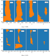 |
Fig. 7 Stability maps (a × e) showing the evolution of the sailboat region for varying particle inclinations in binary systems with mass ratios μ = 0.05 and 0.12. |
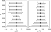 |
Fig. 8 Interval of the particle argument of pericenter where the sailboat region exists with maximum extension at ω = 0° (left plot) and ω = 180° (right plot). |
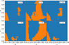 |
Fig. 9 Stability maps (a × e) for a binary system with μ = 0.05 showing the sailboat region evolution across different values of argument of pericenter. Stable initial conditions are shown in orange, unstable in blue. |
6 Stability verification
To validate our machine learning predictions and provide an independent confirmation of the stability patterns identified in this work, we employed two complementary verification methods.
The stability of the sailboat region was demonstrated by Giuliatti Winter et al. (2014), who studied the sailboat region in the Pluto–Charon system and identified its stability through the family BD of periodic orbits described by Broucke (1968). They employed Poincaré surfaces of section (PSS) to confirm the region’s stability. The PSS method is a powerful tool for demonstrating stability by revealing the periodic and quasi-periodic trajectories within a system. However, its effectiveness is limited by its dependence on the Jacobi Constant to reduce the system’s degrees of freedom, a constant that only exists in the circular restricted three-body problem (CRTBP). Additionally, the PSS method’s representation is constrained to the x and vx phase space of a barycentric synodic coordinate system, which can limit the scope of analysis.
To confirm the stability of the regions obtained by the machine learning we present a combination of techniques, including Poincaré surfaces of section (PSS), and the Lyapunov exponent as a chaos indicator. The Lyapunov exponent is a fundamental tool for diagnosing chaos in dynamical systems, as it quantifies the rate at which nearby trajectories diverge, providing a rigorous measure of a system’s sensitivity to initial conditions. This approach has proven particularly effective for studying chaotic behavior in celestial mechanics (Popova & Shevchenko 2013). A positive Lyapunov exponent indicates the exponential divergence of initially close trajectories, which signifies chaos. Conversely, a negative exponent suggests that trajectories converge, indicating stability, while a zero value implies neutral stability. The greater the positive exponent, the more unpredictable the system becomes over time.
In analyzing stochastic regions, it’s crucial to estimate the time-scale for the onset of chaos in orbital motion, which is defined as the Lyapunov time. This is the inverse of the largest Lyapunov characteristic number (LCN). Obtaining an accurate LCN typically requires a long integration time, on the order of 105 to 106 orbital periods. However, this study uses REBOUND with IAS15 (Rein & Spiegel 2015), which employs the Mean Exponential Growth factor of Nearby Orbits (MEGNO) method (Cincotta & Simó 2000). MEGNO provides a measure of chaos that is proportional to the LCN, allowing for its accurate determination in significantly shorter, more realistic physical times of approximately 103 periods (Cincotta & Simó 2000). This approach offers a more efficient way to quantify the chaotic nature of these regions.
Rather than a comprehensive stability study, we focused on validating our machine learning predictions through targeted analysis of specific cases. We selected several representative systems for detailed examination using PSS and LCN. From Figure 2, which depicts a system where the eccentricity of the binary is zero and particles lie in plane x, y, we chose cases with μ = 0.15 and μ = 0.23 for analysis using both PSS and LCN. For the cases presented in Figure 4 (μ = 0.12 and es = 0.023) and Figure 6 (μ = 0.12 and i = 75°), we used only the LCN due to the inherent limitations of PSS in analyzing those specific systems. It is important to note that these calculations have far greater time and computational requirements compared with the machine learning method.
In Figure 10, we present PSS for trajectories located at the boundaries of the sailboat region, as depicted in Figure 2, for a mass ratio of μ = 0.13. We chose three test particles for projection onto the (x, vx) plane, each having distinct Jacobi constants and positions within the sailboat region: one at the far left edge, one at the far right edge, and one in the center. The resulting trajectories correspond to quasi-periodic orbits, and their stability is confirmed by the regular, predictable patterns observed in the surfaces of section. We also illustrate the same region from Figure 2 using the LCN, represented by a color gradient. The logarithmic value of the LCN is plotted, where more negative values indicate less chaotic trajectories. The similarity between the regions of low chaos derived from the LCN and the stability map generated by the machine learning method is remarkable, highlighting the efficiency of the latter, even when accounting for the initial training time.
Figure 11 shows an extreme case where μ = 0.23. Using PSS, we encountered difficulties in finding quasi-periodic orbits, with only one trajectory within the main sailboat region proving stable. Despite this challenge with PSS, the LCN method indicates almost the same region as more stable compared to our machine learning predictions, with the negative logarithm of the LCN being below −4. This implies an LCN below 10−4. This agreement is remarkable given that we trained the machine learning method with trajectories that remained stable for 104 orbital periods (see Section 3.1) and not with LCN values.
When we account for the eccentricity of the binary, we diverge from the CRTBP and the stability of the sailboat regions deteriorates. Our machine learning method demonstrates this effect in Figure 4. The bottom panel of Figure 11 shows the LCN for the same parameter space (μ = 0.12 and es = 0.023). Comparing these results proves more challenging because the LCN regions with more negative values are dispersed. However, the stable region remains predominantly located in the middle of both figures, indicating correspondence between the two methods.
The right panel of Figure 12 shows the region corresponding to Figure 7, with μ = 0.12 and i = 75°. Giuliatti Winter et al. (2013) demonstrated that the stability of the sailboat region extends out of the plane, even up to high inclinations. Our machine learning method also identified this stability and the LCN method shows a region with less chaoticity that is almost compatible. Although this comparison shows the most divergence of the four cases presented, with our machine learning predictions being more symmetric than the LCN results, both methods still reveal similar underlying structures. This indicates that our approach can effectively identify possible regions of stability, even with certain limitations. These discrepancies reveal that while our machine learning approach efficiently maps general stability regions with minimal computational cost, some boundary points might be misclassified.
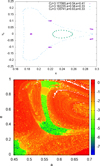 |
Fig. 10 Upper panel: Poincaré surfaces of section in the (x, vx) plane for selected trajectories at the boundaries of the sailboat region with μ = 0.13. Three trajectories correspond to different positions within the sailboat: leftmost edge, center, and rightmost edge. Quasi-periodic orbits appear as closed curves, confirming stability. Bottom panel: map of LCN in the same region for case μ = 0.13. The most negative regions indicate less chaotic trajectories. |
7 Final remarks
The sailboat region is a stable zone for S-type orbits in binary systems. This region lies approximately midway between the two massive bodies and supports particles with highly eccentric orbits reaching e = 0.9. Through stability verification methods including Poincaré surfaces of section and Lyapunov exponent analysis, we confirmed that this stability originates from a family of periodic orbits that persist despite the strong gravitational perturbations typical of binary environments.
In this paper, we studied how the sailboat region responds to changes in binary system parameters. We studied four key parameters: binary mass ratio, secondary body eccentricity, particle orbital inclination, and argument of pericenter. We combined direct numerical integration of 1.2 million three-body systems with machine learning algorithms. This approach allowed us to predict stability for about 109 initial conditions with an accuracy exceeding 97%.
Our analysis reveals that the sailboat region exists exclusively within a limited mass ratio range, μ = [0.05, 0.22]. Below μ = 0.05, the region connects with the inner stable zone around the primary body. For μ > 0.22, gravitational perturbations eliminate all stability in this parameter space. Within this range, higher μ values make the sailboat region smaller and closer to the primary body, while requiring higher minimum eccentricities.
The secondary body’s eccentricity severely constrains sailboat region existence, in a way that even small increases from circular orbits rapidly destabilize the region, following an exponential decay relationship. For μ = 0.05, the maximum secondary eccentricity is about 0.23, but drops to only 0.007 for μ = 0.22. This strong dependence means that most binary systems with eccentric components cannot support stable sailboat regions.
Particle inclination shows good tolerance, with the sailboat region surviving inclinations from 0° to 90° for most mass ratios. Retrograde configurations can still support sailboat stability when μ ≤ 0.16, although with a reduced spatial extent. This inclination tolerance increases the number of possible systems where such regions might exist.
The argument of pericenter creates strong limits on sailboat region existence. Stability occurs only within narrow angular ranges: Δω ≈ ±10° to ±30° centered at ω = 0° and ω = 180°. This selectivity comes from the periodic orbit family needing specific orientations relative to the binary axis. Nevertheless, the method provides a valuable tool for initial stability surveys, significantly reducing computational requirements for comprehensive dynamical studies. Once trained, our machine learning model can reduce computation time up to a factor of 105 compared to numerical simulations. For instance, it takes about a couple of months using a single core with typical specifications to build the training dataset, whereas the model training and ML prediction take an order of several seconds to run. This performance allows us to explore orbital stability across large parameter spaces, although detailed investigations remain necessary to confirm the real stability of identified regions.
These results can be applied to several real systems. Among the dwarf planet binaries in our Solar System, such as the Pluto–Charon, Orcus–Vanth, and Varda-Ilmarë systems, have mass ratios and eccentricities that could support sailboat regions. These systems are good targets for searching for ring structures or small satellites in such regions. Our results also help with spacecraft mission planning in binary environments by identifying stable parking orbits and regions that require trajectory changes.
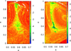 |
Fig. 12 Lyapunov exponents for regions explored by the ML. Left: region of Figure 5 (μ = 0.12 and es = 0.023). Right: region of Figure 7 (μ = 0.12 and i = 75°). |
Acknowledgements
We thank the reviewer for their insightful comments and valuable suggestions. R.S. acknowledge support by the DFG German Research Foundation (project 446102036) and CNPq (307400/2025-5). E.V.N thans CNPq (309105/2022-6). R.S. and G. R. are grateful to the São Paulo Research Foundation (FAPESP, grant 2024/20150-1). T.F.L.L.P. acknowledge support from the Conselho Nacional de Desenvolvimento Científico e Tecnológico (CNPq) – Proc.313994/2025-0. The authors thank the Improvement Coordination Higher Education Personnel – Brazil (CAPES) – Financing Code 001.
References
- Bondarenko, I., & Perevozkina, E. 2004, VizieR Online Data Catalog: V/120 [Google Scholar]
- Broucke, R. A. 1968, Periodic orbits in the restricted three-body problem with earth-moon masses [Google Scholar]
- Brown, M. E., & Butler, B. J. 2023, Planet. Sci. J., 4, 193 [Google Scholar]
- Brozović, M., & Jacobson, R. A. 2024, AJ, 167, 256 [Google Scholar]
- Chawla, N. V., Bowyer, K. W., Hall, L. O., & Kegelmeyer, W. P. 2002, J. Artif. Intell. Res., 16, 321 [CrossRef] [Google Scholar]
- Cincotta, P. M., & Simó, C. 2000, A&AS, 147, 205 [NASA ADS] [CrossRef] [EDP Sciences] [Google Scholar]
- Géron, A. 2022, Hands-on Machine Learning with Scikit-Learn, Keras, and TensorFlow (O’Reilly Media, Inc.) [Google Scholar]
- Giuliatti Winter, S., Winter, O., Vieira Neto, E., & Sfair, R. 2013, MNRAS, 430, 1892 [NASA ADS] [CrossRef] [Google Scholar]
- Giuliatti Winter, S. M., Winter, O., Vieira Neto, E., & Sfair, R. 2014, MNRAS, 439, 3300 [Google Scholar]
- Grundy, W. M., Porter, S. B., Benecchi, S. D., et al. 2015, Icarus, 257, 130 [NASA ADS] [CrossRef] [Google Scholar]
- Grundy, W., Noll, K., Roe, H., et al. 2019, Icarus, 334, 62 [CrossRef] [Google Scholar]
- Hastie, T., Tibshirani, R., Friedman, J. H., & Friedman, J. H. 2009, The Elements of Statistical Learning: Data Mining, Inference, and Prediction, 2 (Springer) [Google Scholar]
- He, H., Bai, Y., Garcia, E. A., & Li, S. 2008, in 2008 IEEE International Joint Conference on Neural Networks (IEEE World Congress on Computational Intelligence) (IEEE), 1322 [Google Scholar]
- Holler, B., Grundy, W., Buie, M., & Noll, K. 2021, Icarus, 355, 114130 [NASA ADS] [CrossRef] [Google Scholar]
- Kiss, C., Marton, G., Parker, A. H., et al. 2019, Icarus, 334, 3 [NASA ADS] [CrossRef] [Google Scholar]
- Kopal, Z. 1955, Ann. Astrophys., 18, 379 [Google Scholar]
- Morgado, B., Sicardy, B., Braga-Ribas, F., et al. 2023, Nature, 614, 239 [NASA ADS] [CrossRef] [Google Scholar]
- Ortiz, J. L., Santos-Sanz, P., Sicardy, B., et al. 2017, Nature, 550, 219 [NASA ADS] [CrossRef] [Google Scholar]
- Pereira, C., Sicardy, B., Morgado, B., et al. 2023, A&A, 673, L4 [NASA ADS] [CrossRef] [EDP Sciences] [Google Scholar]
- Pinheiro, T. F., Sfair, R., & Ramon, G. 2025, A&A, 693, A246 [NASA ADS] [CrossRef] [EDP Sciences] [Google Scholar]
- Popova, E. A., & Shevchenko, I. I. 2013, ApJ, 769, 152 [NASA ADS] [CrossRef] [Google Scholar]
- Ragozzine, D., & Brown, M. E. 2009, AJ, 137, 4766 [NASA ADS] [CrossRef] [Google Scholar]
- Rein, H., & Spiegel, D. S. 2015, MNRAS, 446, 1424 [Google Scholar]
- Shalev-Shwartz, S., & Ben-David, S. 2014, Understanding Machine Learning: From Theory to Algorithms (Cambridge University Press) [Google Scholar]
- Sheppard, S. S., Fernandez, Y. R., & Moullet, A. 2018, AJ, 156, 270 [Google Scholar]
- Surkova, L., & Svechnikov, M. 2004, VizieR Online Data Catalog: V/115 [Google Scholar]
- Svechnikov, M., & Perevozkina, E. 2004, VizieR Online Data Catalog: V/124 [Google Scholar]
- Tamayo, D., Silburt, A., Valencia, D., et al. 2016, ApJ, 832, L22 [NASA ADS] [CrossRef] [Google Scholar]
- Wade, C., & Glynn, K. 2020, Hands-On Gradient Boosting with XGBoost and scikit-learn: Perform accessible machine learning and extreme gradient boosting with Python (Packt Publishing Ltd) [Google Scholar]
- Weerts, H. J., Mueller, A. C., & Vanschoren, J. 2020, arXiv preprint [arXiv:2007.07588] [Google Scholar]
- Winter, O., & Vieira Neto, E. 2001, A&A, 377, 1119 [NASA ADS] [CrossRef] [EDP Sciences] [Google Scholar]
- Winter, S. G., Winter, O., Guimarães, A. F., & Silva, M. 2010, MNRAS, 404, 442 [Google Scholar]
All Tables
All Figures
|
Fig. 1 Diagram of a binary star system (d × μ), where d represents the separation distance between the stars and μ is the binary mass ratio. The diagram categorizes the binary types as follows: blue for detached, green for semidetached, and red for contact. The black point corresponds to the Pluto–Charon system. |
| In the text | |
|
Fig. 2 Stability maps in the (a, e) plane for binary systems with mass ratios μ = [0.01–0.23]. Stable initial conditions are shown in orange, unstable in blue. All particles are in coplanar orbits around the primary body with ω = Ω = f = 0°. |
| In the text | |
|
Fig. 3 Sailboat region for a binary system with μ = 0.12 (the closest case with Pluto–Charon system, where Charon has eccentricity). The red dashed line represents the pericenter of the particle in the same distance of Pluto’s radius. There is other stable regions in the range a = [0.45–0.7], not showed in the plot. |
| In the text | |
|
Fig. 4 Maximum eccentricity of secondary body (blue dots) versus mass ratio of the system. The red curve represents a fitted model obtained using the least squares method. Green squares denote binary systems of dwarf planets and their satellites, while the black square represents the Pluto–Charon system. |
| In the text | |
|
Fig. 5 Stability maps (a × e) showing the evolution of the sailboat region with changing secondary body eccentricity for binary systems with mass ratios of μ = 0.05, 0.12, and 0.22. |
| In the text | |
|
Fig. 6 Stability regions for different particle orbital inclinations. Orange areas indicate inclination values where stable regions exist within a = [0.4–0.7] for various μ. The gaps in coverage indicate parameter combinations where the sailboat region becomes unstable. |
| In the text | |
|
Fig. 7 Stability maps (a × e) showing the evolution of the sailboat region for varying particle inclinations in binary systems with mass ratios μ = 0.05 and 0.12. |
| In the text | |
|
Fig. 8 Interval of the particle argument of pericenter where the sailboat region exists with maximum extension at ω = 0° (left plot) and ω = 180° (right plot). |
| In the text | |
|
Fig. 9 Stability maps (a × e) for a binary system with μ = 0.05 showing the sailboat region evolution across different values of argument of pericenter. Stable initial conditions are shown in orange, unstable in blue. |
| In the text | |
|
Fig. 10 Upper panel: Poincaré surfaces of section in the (x, vx) plane for selected trajectories at the boundaries of the sailboat region with μ = 0.13. Three trajectories correspond to different positions within the sailboat: leftmost edge, center, and rightmost edge. Quasi-periodic orbits appear as closed curves, confirming stability. Bottom panel: map of LCN in the same region for case μ = 0.13. The most negative regions indicate less chaotic trajectories. |
| In the text | |
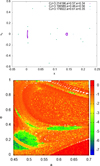 |
Fig. 11 Same as Figure 10 for μ = 0.23. |
| In the text | |
|
Fig. 12 Lyapunov exponents for regions explored by the ML. Left: region of Figure 5 (μ = 0.12 and es = 0.023). Right: region of Figure 7 (μ = 0.12 and i = 75°). |
| In the text | |
Current usage metrics show cumulative count of Article Views (full-text article views including HTML views, PDF and ePub downloads, according to the available data) and Abstracts Views on Vision4Press platform.
Data correspond to usage on the plateform after 2015. The current usage metrics is available 48-96 hours after online publication and is updated daily on week days.
Initial download of the metrics may take a while.