| Issue |
A&A
Volume 703, November 2025
|
|
|---|---|---|
| Article Number | A225 | |
| Number of page(s) | 13 | |
| Section | Interstellar and circumstellar matter | |
| DOI | https://doi.org/10.1051/0004-6361/202555944 | |
| Published online | 18 November 2025 | |
High-resolution models of the vertical shear instability
1
Univ. Grenoble Alpes, CNRS,
IPAG,
38000
Grenoble,
France
2
Department of Applied Mathematics and Theoretical Physics, Centre for Mathematical Sciences, University of Cambridge,
Wilberforce Road, Cambridge CB3 0WA,
UK
★ Corresponding author: This email address is being protected from spambots. You need JavaScript enabled to view it.
Received:
13
June
2025
Accepted:
8
August
2025
Abstract
Context. The vertical shear instability (VSI) is a promising mechanism for generating turbulence and transporting angular momentum in magnetically decoupled regions of protoplanetary discs. While most recent work has focused on adding more complex physics, the saturation properties of the instability in radially extended discs, and its convergence as a function of resolution, are still largely unknown.
Aims. We address the question of VSI saturation and associated turbulence using radially extended, fully 3D global disc models with very high resolution in the locally isothermal approximation, to capture both the largest VSI scales and the small-scale turbulent cascade.
Methods. We used the GPU-accelerated code Idefix to achieve resolutions of up to 200 points per scale height in the three spatial directions. We chose numerical techniques that minimise numerical diffusion as much as possible: third-order reconstruction schemes, orbital advection, and a third-order time integrator. We modelled the VSI in disc domains extending up to Rout/Rin = 7 in the highest resolution case and Rout/Rin = 25 in our intermediate model (100 points per scale height), with a full 2 π azimuthal extent and a disc aspect ratio H/R = 0.1.
Results. We demonstrate that large-scale transport properties converge with 100 points per scale height, leading to a Shakura-Sunyaev α=1.3 × 10⁻³ in the bulk of the computational domain. Inner boundary condition artefacts propagate deep inside the computational domain (typically over Δ R/R ∼ 2−3), leading to a reduced α in these regions. The large-scale corrugation wave zones identified in 2D models persist in 3D, albeit with less coherence. Our models show no signs of long-lived zonal flows, pressure bumps, or vortices, in contrast to lower-resolution simulations. Finally, we show that the turbulent cascade resulting from VSI saturation can be interpreted within the framework of critically balanced rotating turbulence. We propose that the small non-axisymmetric scales could be modelled with an effective anisotropic viscosity in 2D simulations, significantly reducing the computational cost of these models while still capturing the important physics.
Conclusions. The VSI leads to vigorous turbulence in protoplanetary discs, associated with outward angular momentum transport, but without any significant long-lived features that could enhance planet formation. The innermost regions of VSI simulations are consistently polluted by boundary-condition artefacts influencing the first VSI wave train. Radially extended domains should therefore be used in a more systematic manner, and more realistic inner boundaries should be explored to mimic the radial structure of real protoplanetary discs.
Key words: hydrodynamics / turbulence / protoplanetary disks
© The Authors 2025
 Open Access article, published by EDP Sciences, under the terms of the Creative Commons Attribution License (https://creativecommons.org/licenses/by/4.0), which permits unrestricted use, distribution, and reproduction in any medium, provided the original work is properly cited.
This article is published in open access under the Subscribe to Open model. This email address is being protected from spambots. You need JavaScript enabled to view it. to support open access publication.
1 Introduction
The vertical shear instability (VSI) has emerged as a prominent hydrodynamic mechanism capable of generating turbulence in regions of protoplanetary discs where magnetic activity is weak or absent, a region usually referred to as the dead zone. First identified in the early work of Urpin & Brandenburg (1998), the VSI gained substantial attention following the seminal study by Nelson et al. (2013), which demonstrated its robust development in locally isothermal discs. The instability is now recognised as a manifestation of the Goldreich-Schubert-Fricke (GSF) instability, originally formulated in the context of stellar interiors (Goldreich & Schubert 1967; Fricke 1968), and is driven by vertical shear in the angular velocity profile under conditions of efficient cooling.
Since then, linear analyses have clarified the conditions under which the VSI can grow, with key contributions from Barker & Latter (2015) and Lin & Youdin (2015). The nonlinear saturation of the VSI has been explicitly addressed through 2D (Flores-Rivera et al. 2020) and 3D (Manger et al. 2020; Shariff & Umurhan 2024) simulations and is believed to result either from delayed Kelvin–Helmholtz instabilities (Latter & Papaloizou 2018) or from parametric instabilities (Cui & Latter 2022).
Most recent work on VSI has focused on adding new physics. For example, studies have examined the interaction of VSI with magnetohydrodynamics (MHD) and with the magneto-rotational instability (Latter & Papaloizou 2018; Cui & Bai 2020; Latter & Kunz 2022; Cui & Bai 2022); thermodynamic improvements, such as the inclusion of radiative transfer with M1 closure schemes (Melon Fuksman et al. 2024a), and more realistic vertical disc structures (Zhang et al. 2024); and finally, the impact of VSI on dust grain dynamics (Flock et al. 2017; Dullemond et al. 2022; Pfeil et al. 2023), together with the feedback of the grains’ inertia on the VSI (Huang & Bai 2025b).
Despite this additional complexity, many basic questions remain regarding the long-term saturation and energy cascade of the VSI. Notably, one of the defining features of the VSI is its ability to excite a type of large-scale inertial wave, known as ‘corrugation modes’, which can dominate the vertical and radial dynamics of the disc (Nelson et al. 2013; Stoll & Kley 2014). These corrugation modes form wave trains that develop into well-defined radial wave zones in 2D simulations (Svanberg et al. 2022). However, capturing several of these wave trains is notoriously difficult, as this requires radially extended simulation domains. The only studies that clearly exhibit several wave trains are axisymmetric (Stoll & Kley 2014; Svanberg et al. 2022), with rout/rin>10, while all 3D simulations published to date have rout/rin<5 (cf. Table 1).
This question of radial extent is important because VSI is an instability of inertial waves travelling radially outwards (Ogilvie et al. 2025). Consequently, the innermost travelling wave packet is necessarily affected by the inner boundary condition of the domain, a problem that has been largely overlooked in the community. However, there are hints that some boundary artefacts are present: Shariff & Umurhan (2024) show that the turbulent transport parameter α increases linearly with radius in a box with rout/rin = 2, a rather unexpected result if the VSI and its saturation were truly a radially local process. Thus, how the VSI saturates in a truly radially extended domain remains an open question.
Other questions of interest include whether the saturation mechanism involves the formation of long-lived structures such as zonal flows and vortices, which might trap dust grains and trigger planet formation (Richard et al. 2016; Manger & Klahr 2018; Pfeil & Klahr 2021). Finally, the nature of the turbulent cascade is also debated, as various studies report different phenomenologies (Manger & Klahr 2018; Shariff & Umurhan 2024; Melon Fuksman et al. 2024a), ranging from direct Kolmogorov cascades to quasi-2D inverse cascades.
The goal of this work is to address the problem of VSI saturation in a sufficiently large domain to capture several corrugation wave zones, while at the same time ensuring sufficient resolution to adequately describe the small-scale turbulent cascade, thus providing a complete picture of VSI saturation. The models also need to be 3D to capture the possible breakup of zonal flows into vortices. The requirement for several wave zones translates into rout/rin ∼ 20, while adequately capturing VSI saturation requires about 100 points per disc pressure scale height in 2D models (Flores-Rivera et al. 2020), a constraint that we will assume to be valid in 3D. Combining these constraints implies simulations with 1010−1011 cells (i.e. about 400 times more cells than the most recent 3D models of Shariff & Umurhan 2024), making optimised numerical techniques and GPU acceleration mandatory.
In the following sections, we first present the numerical techniques and setup used. We then present the main results of our models and finally discuss its implications.
Previous studies and their models’ key properties, including the number of dimensions D, radial aspect ratio, number of grid points n per disc scale height H and azimuthal extent Δ φ.
2 Methods
2.1 Physical setup
The setup consists of a locally isothermal disc with density ρ ∝ R−3/2, or equivalently surface density Σ ∝ R−1/2, and an aspect ratio H/R = 0.1 such that the sound speed is cs = 0.1 vK, where vK is the Keplerian velocity. To capture radially extended structures, we considered simulations with radially extended domains. We constructed two simulations with rout/rin = 25 at resolutions of 40 and 80 points per scale height (runs LX and HX), and a higher-resolution simulation with a reduced radial extension Rout/Rin = 7, but an extreme resolution of 200 points per scale height (run EX). All of the simulations extended vertically over ± 4 pressure scale heights (θ−π/2 in[−0.4,+0.4]) and over 2 π in the azimuthal direction. We used a logarithmic spacing for the radial grid, while keeping a constant spacing in θ and φ, which ensured that the cell size per H remained homogeneous throughout the domain.
We designed the radial boundary conditions to avoid wave reflection and to limit boundary artefacts as much as possible. At the boundary itself, we enforced an outflow condition, where the tangential velocity is copied into the ghost cells, while the normal velocity is either copied (when directed outside of the computational domain) or set to zero. The density and pressure are extrapolated from the last active zone assuming hydrostatic equilibrium power laws (see below). We supplemented the radial boundary condition with a radial wave-killing zone in which the density, pressure, and velocity are relaxed towards the equilibrium values on a characteristic timescale equal to the local orbital timescale. These wave-killing zones extend radially over two local pressure scale heights on both sides of the domain.
The meridional boundary conditions are stress-free: the flow is not allowed to escape the domain, and the tangential velocity components are copied from the last active cell in the ghost cells. The density and pressure are extrapolated from the last active cell, assuming hydrostatic equilibrium. Finally, the flow is assumed to be periodic in the azimuthal direction.
We started simulation LX from a hydrostatic equilibrium (Nelson et al. 2013) on top of which we added a low-level random noise δ v/VK = 10−4. We restarted the higher-resolution simulations HX and EX from a snapshot taken at t = 1000 orbits after the beginning of run LX, interpolating the field values onto the higher-resolution grid. This procedure allowed us to minimise the long transient preceding VSI saturation observed in run LX for the first 250 orbits. The run properties are summarised in Table 2.
2.2 Numerical technique
The overarching goal of our numerical setup is to limit numerical dissipation, in order to resolve the VSI’s secondary instabilities and the resulting turbulent cascade as accurately as possible. We performed all simulations presented here using the Idefix code (Lesur et al. 2023) with a compact third-order reconstruction scheme (Čada & Torrilhon 2009, LiMO3) and the Harten-Lax-van Leer-Contact (HLLC) Riemann solver. To limit numerical dissipation due to advection by Keplerian rotation, we used the orbital advection scheme (also known as ‘Fargo’) implemented in Idefix in a fully conservative manner (Mignone et al. 2012), using a piecewise parabolic (PPM) method to reconstruct fractional advection. The system of equations is evolved using a third-order TVD Runge–Kutta scheme.
Main properties of simulations presented in the paper.
We ran the code on the LUMI-G pre-exascale supercomputer in Finland, using 4096 AMD Mi250X GPUs simultaneously for the two highest-resolution models.
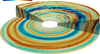 |
Fig. 1 Three-dimensional rendering of the meridional velocity sonic Mach number vθ/cs in simulation EX (200 points per H) at t = 800 orbits after restart. The front part shows the flow in the midplane, while the back part shows the flow at 3 H above the midplane, with numerical boundaries at 4 H. The domain has been truncated at Rout = 5.6 to remove the outer wave-killing zone. |
2.3 Units and diagnostics
For all models, we use the inner radius as the length unit, while the Keplerian velocity at the inner radius serves as the velocity unit. The azimuthal average of a 3D quantity Q is denoted 〈Q〉, the time average of a quantity is given by 〈Q〉t (taken over the entire simulation time unless otherwise specified), and the azimuthal and vertical average over three scale heights H is denoted by Q̄, defined through the meridional angle  :
:
 (1)
(1)
The azimuthal average defines the non-axisymmetric deviation for each field as v′=v−〈v〉. Finally, the Keplerian velocity profile is assumed to be constant on cylinders, i.e. vK(r, θ)= (r sin θ)−1/2. This is used to define the deviation from Keplerian rotation, δ v(r, θ, φ)=v−vK eφ.
3 Results
3.1 Overview
The main features of our simulations can be identified in the instantaneous snapshot shown in Fig. 1, which shows the 3D latitudinal velocity vθ of the highest-resolution model EX taken after 800 inner orbits. The flow exhibits large-scale, quasi-axisymmetric upward and downward motion visible as ‘bands’. In addition, the surface exhibits numerous fine-scale structures on top of these bands. We focus on each of these features in turn and demonstrate how they are connected.
3.2 Time history and bulk transport properties
The temporal evolution of the angular momentum transport coefficient α and turbulent poloidal energy ek is first considered; these are defined as
 (2)
(2)
 (3)
(3)
These quantities, measured at R = 4 in simulations LX, HX, and EX, are shown in Fig. 2. The LX simulation exhibits transient growth from 0 to saturation for the first 300 orbits. This initial transient corresponds to the linear growth and saturation of the VSI. It is absent in the HX simulation because this run is initialised from the saturated state of LX. All simulations converge to the same steady state with 〈α〉t = 1.3 × 10⁻³ and 〈eK〉t = 1.9 × 10⁻² when averaged over the 1000 orbits, indicating that the bulk transport properties converge with resolution in these simulations. The instantaneous α oscillates widely between ± 10−2, and only after applying a 20-orbit running mean is the long-time average recovered.
Fig. 3 shows the radial dependence of the transport properties. We excised the radial buffer zones used to damp wave reflections to ensure that this figure accurately reflects the ‘active domain’ of the simulations. The transport properties increase gradually between R = 1.2 and R = 4 where they reach a plateau. This feature is present in all of the models with the same amplitude, indicating convergence with spatial resolution. However, this behaviour is incompatible with the self-similar disc assumption, for which constant dimensionless values would be expected. This observation therefore likely indicates the influence of the inner boundary condition, which propagates deep (Δ R ∼ 20 H) inside the active domain. For R>4, all models appear perfectly self-similar and show values similar to the time averages in Fig. 2.
The average value of 〈α〉t at R = 4 (Fig. 2) is about twice the value reported in the 3D models of Shariff & Umurhan (2024) and approximately 30% larger than that reported by Manger & Klahr (2018). This discrepancy is probably due to the more extended radial domain used in our simulations. At R = 1.5, 〈α〉t ∼ 5 × 10⁻⁴, a value compatible with that reported by Manger & Klahr (2018), but still significantly larger than Shariff & Umurhan (2024).
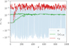 |
Fig. 2 Radial angular momentum coefficient (α) and poloidal kinetic energy (ek) measured at R = 4 in run HX (solid line) and run LX (dashed line). For clarity, we show the instantaneous α and the time-averaged α over a window of 20 local orbits, 〈α〉t, 20. Run HX was initialized from the saturated state of LX, which explains the absence of an initial transient in HX. |
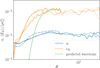 |
Fig. 3 Angular momentum transport and poloidal kinetic energy (ek) averaged over the last 400 orbits of the simulations EX (solid line), HX (dashed line), and LX (dotted line). The predicted amplification and saturation radius for a single linear wave train with frequency ω=0.075 Ω0 and n = 1 from Ogilvie et al. (2025) is shown as a dashed green line (Eq. (5)). |
3.3 Flow structure
The instantaneous flow shape appears in an R−z cut at a fixed azimuth (Fig. 4). Large corrugation n = 1 modes (Ogilvie et al. 2025) are recovered, characterised by a column moving vertically up or down uniformly, alongside horizontal oscillations antisymmetric with respect to the disc midplane. In addition to these structures, we observe fine-scale structures and shocks, the latter being particularly evident in vR and ρ. The velocity magnitude is clearly sonic at three scale heights, which explains the presence of moderately strong (δ ρ/ρ ∼ 1) density jumps in the flow, especially visible in the disc atmosphere (|z| ≳ 0.2 R = 2 H).
The R−φ cuts (Fig. 5) reveal large-scale vz motions that remain remarkably axisymmetric in the disc midplane. In the disc atmosphere, at 3 H, large-scale vertical motion becomes stronger, but non-axisymmetric structures are also much more pronounced. Small-scale eddies, which resemble radial mixing of vz, and oblique shocks, are distinguishable. These shocks become apparent in the density at z = 3 H (Fig. 5 bottom), where trailing non-axisymmetric shocks appear throughout the simulation domain.
3.4 Zonal flows
The appearance of long-lived zonal flows in the context of VSI turbulence has been proposed in several studies (e.g. Richard et al. 2016; Manger & Klahr 2018). Such zonal flows could prevent the inward migration of centimetre-sized dust grains, a problem historically known as the metre barrier (Weidenschilling 1977). For these zonal flows to act as efficient dust traps, they must generate pressure bumps; that is, the flow should become locally super-Keplerian.
Fig. 6 presents the relative deviation from the Keplerian velocity in the disc midplane for run HX, where two strong zonal flows appear close to the inner (R ≃ 1.2) and outer (R ≃ 21) radial boundaries. These features are clearly boundary condition artefacts and should be disregarded. In the bulk of the disc, weak deviations from Keplerian rotation are present but never exceed 1%, and the flow remains on average Keplerian.
This absence of strong zonal flows may be related to the flow symmetry with respect to the disc midplane (Fig. 4). In particular, we find that δ vφ is always antisymmetric with respect to z = 0. This antisymmetry of δ vφ, together with the symmetry of vz, is characteristic of the n = 1 corrugation mode (Ogilvie et al. 2025), and we confirm this mode selection in Section 3.5. These observations indicate that deviations from Keplerian rotation in the disc midplane are weak and insufficient to feed long-lived pressure bumps or dust traps.
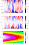 |
Fig. 4 Instantaneous (R, z) cut of the HX model at t = 900 orbits. Large-scale n = 1 corrugation modes are evident in vz, reaching sonic velocities (top panel), along with shock fronts propagating radially in the density field (bottom panel). |
3.5 Large-scale wave propagation
As discussed above, we recover the large-scale n = 1 corrugation modes identified in 2D simulations (Stoll & Kley 2014; Svanberg et al. 2022). These are clearly visible in the space-time diagram of the mean vertical mass flux  (Fig. 7). The diagram reveals several wave zones with temporal and spatial frequencies.
To better diagnose these properties, we first measured the radial wavelength of the corrugation pattern between two nulls of  at each time in the HX simulation. This provided us with a distribution of radial wavelengths at each radius (Fig. 8). The figure reveals four wave regions, each following the linear dispersion relation of an n = 1 inertial mode with a fixed frequency ω:
 (4)
where Ω is the local Keplerian frequency, cs is the local isothermal sound speed, and k = 2 π/λ is the radial wavenumber (Lubow & Pringle 1993; Ogilvie et al. 2025). We fit the wave regions in Fig. 8, using the frequencies ω/Ω0 = 0.075, 0.025, 0.0094, and 0.0041 (where Ω0 ≡ Ω(R = 1)), representing a best fit ‘by eye’ to the data. These inertial waves appear when ω<Ω and possess a Lindblad resonance at R = RL, which satisfies ω=Ω(RL); beyond this point, they become (stable) acoustic waves. In our simulations, the wave trains tend to vanish as they approach their respective resonances and are replaced by lower-frequency wave trains. A very steep band of short waves near the inner boundary provides further evidence of inner boundary artefacts.
(4)
where Ω is the local Keplerian frequency, cs is the local isothermal sound speed, and k = 2 π/λ is the radial wavenumber (Lubow & Pringle 1993; Ogilvie et al. 2025). We fit the wave regions in Fig. 8, using the frequencies ω/Ω0 = 0.075, 0.025, 0.0094, and 0.0041 (where Ω0 ≡ Ω(R = 1)), representing a best fit ‘by eye’ to the data. These inertial waves appear when ω<Ω and possess a Lindblad resonance at R = RL, which satisfies ω=Ω(RL); beyond this point, they become (stable) acoustic waves. In our simulations, the wave trains tend to vanish as they approach their respective resonances and are replaced by lower-frequency wave trains. A very steep band of short waves near the inner boundary provides further evidence of inner boundary artefacts.
Fig. 9. shows the directly measured temporal spectrum of the corrugation waves. The spectrum displays horizontal bands grouped into broader structures. Each horizontal band corresponds to a particular wave frequency excited over a range of radii. The dotted line corresponds to the best-fit frequencies mentioned above and approximately fits the large bumps in the structures. However, the temporal spectrum is much broader in frequency than in 2D (Svanberg et al. 2022). This is possibly due to small-scale turbulence, which excites additional modes of flow. Surprisingly, we recover the same wave frequencies (within 10%) as those found in 2D simulations, indicating that the VSI somehow selects those particular frequencies.
It is tempting to associate the increase in kinetic energy and transport (Fig. 3) observed over 1<R<4 with the amplification of the first wave train. Using a linear analysis, Ogilvie et al. (2025) proposed that the amplitude of a single wave train increases with R according to
 (5)
Fig. 3 shows this prediction for the frequency of our first wave train and reveals that linear theory largely overestimates the radial growth of the wave train. This mismatch may originate from (1) the wave train having already saturated non-linearly and thus is subject to a non-linear viscous damping due to non-axisymmetric structures (cf. Section 3.8), which is absent from the linear analysis of Ogilvie et al. (2025); or (2) the inner wave train is not strictly monochromatic (see Fig. 9), and we are witnessing a combination of radial growth from a spread of wave trains. The radius at which ek saturates matches the plateau of the linear theory. Whether this match constitutes a coincidence or a success of the linear theory remains unclear; a more systematic exploration of the parameter space is necessary to confirm this conjecture.
(5)
Fig. 3 shows this prediction for the frequency of our first wave train and reveals that linear theory largely overestimates the radial growth of the wave train. This mismatch may originate from (1) the wave train having already saturated non-linearly and thus is subject to a non-linear viscous damping due to non-axisymmetric structures (cf. Section 3.8), which is absent from the linear analysis of Ogilvie et al. (2025); or (2) the inner wave train is not strictly monochromatic (see Fig. 9), and we are witnessing a combination of radial growth from a spread of wave trains. The radius at which ek saturates matches the plateau of the linear theory. Whether this match constitutes a coincidence or a success of the linear theory remains unclear; a more systematic exploration of the parameter space is necessary to confirm this conjecture.
3.6 Large-scale vortices
As discussed in Sect. 3.3, the large-scale corrugation motions are accompanied by small-scale structures, which are particularly visible at 3 H (Fig. 5 middle), but are also present in the disc mid-plane. A key question for planet formation theories is the nature of these small-scale structures and the potential emergence of large-scale vortices, which may aid in the assembly of planetary embryos. Such vortices have been found in the 3D simulations of Richard et al. (2016) and were attributed to a local manifestation of the Rossby wave instability (RWI; Lovelace et al. 1999).
We therefore searched for large-scale vortices in the disc midplane. The midplane appears remarkably quiet in terms of vertical velocity (Fig. 5, top), with most chaotic motions occurring in the disc atmosphere. A standard tracer for vortices is the deviation in vertical vorticity δ ωz = r−1[∂r(r δ vφ)−∂φ δ vr], where the background vorticity of the mean Keplerian shear was subtracted. The vertical vorticity is shown in Fig. 10 and reveals numerous small-scale fluctuations that are much smaller than the disc scale height. These fluctuations are highly dynamical (i.e. they evolve on timescales shorter than the local orbital timescale) and do not exhibit any preferential direction with respect to the disc rotation axis. These results stand in sharp contrast to those of Richard et al. (2016) and Manger & Klahr (2018) (hereafter MK18), who both observed the formation of long-lived anticyclonic vortices (i.e., δ ωz Ω<0) at scales ∼ H.
The reason for the absence of long-lived vortices in the high-resolution models is not entirely clear, but several hypotheses can be proposed. First, the resolution is much higher than in Richard et al. (2016) (50 points/H, depending on the direction) and in MK18 (20 points /H). In addition, we used a high-order reconstruction scheme (LimO3) and orbital advection with parabolic reconstruction to minimise numerical dissipation. As a result, our models are able to capture thinner structures that could disrupt large-scale vortices, such as elliptical instabilities (Lesur & Papaloizou 2009). A similar absence of vortices is observed in the high-resolution models (80 points / H) of Shariff & Umurhan (2024), whereas Huang & Bai (2025b) report vortices at lower resolution (30 points / H), supporting the idea of a resolution effect. A second point of difference lies in the cooling timescale, which is infinitely small, as we employed the locally isothermal approximation. Richard et al. (2016) observed that the vortex aspect ratio and lifetime both increase with increasing cooling time. We might therefore be witnessing the breakup of the strongest vortices found by Richard et al. (2016), while weaker vortices at longer cooling timescales (not explored here) might still be present at high resolution.
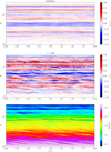 |
Fig. 5 Instantaneous (R, φ) cuts of vertical velocity (vz) and density (ρ) in the HX model at t = 900 orbits. Top: midplane cut of vz. Middle: z = 0.3 R (corresponding to 3 pressure scale heights) cut of vz. Bottom: z = 0.3 R cut of the gas density ρ. |
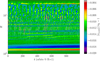 |
Fig. 6 Spatio-temporal evolution of the azimuthally averaged midplane δ vφ/vK in run HX. Weak zonal flows are observed, with deviations from Kepler of the order of 1%. The flow remains sub-Keplerian in the mid-plane throughout the run. |
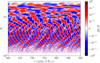 |
Fig. 7 Spatio-temporal evolution of the mean vertical mass flux averaged over φ and θ in simulation HX. Characteristic wave patterns of large-scale corrugation modes, first identified in 2D simulations, are recovered. |
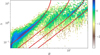 |
Fig. 8 Radial wavelength probability distribution of the large-scale vertical corrugation motion versus R in run HX, computed over the entire simulation duration. Over-plotted in red are the expected frequency of n = 1 inertial modes for frequencies ω/Ω0 = 0.075, 0.025, 0.0094, and 0.0041. |
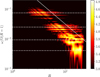 |
Fig. 9 Temporal spectrum of the large-scale vertical corrugation motion versus R in run HX. The dotted lines show the frequencies of the inertial modes plotted in Fig. 8 (ω/Ω0 = 0.075, 0.025, 0.0094., and 0.0041), and the solid line indicates the Keplerian frequency ω=ΩK. |
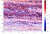 |
Fig. 10 Snapshot of the vertical vorticity perturbation in simulation EX at t = 800 orbits in the disc midplane, zooming in of the region around R = 4.5. The image illustrates the complex turbulent flow and the absence of any large-scale coherent vortical structures. |
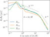 |
Fig. 11 Power spectrum of kinetic energy obtained by integrating the 3D spectrum over spherical shells for each velocity field component at the middle of the computational domain in run EX (see text). |
3.7 Spectra of the small-scale turbulence
The fine-scale structures, being 3D and transient, can be interpreted as manifestations of small-scale (<H) turbulence. To explore this idea, we assessed whether this turbulence can be described within a ‘standard’ fluid-turbulence framework. To this end, we computed the 3D shell-integrated spectrum of run EX, shown in Fig. 11. This spectrum was obtained by extracting a cubic box from run EX centred on R0 = 4 spanning r ∈[3.0, 5.0]; θ−π/2 ∈[−0.2,+0.2]; φ ∈[0, 0.6], running a 3D Fast Fourier transform using a Hanning window, and computing the total kinetic energy in each spherical shell of the resulting spectrum. This procedure allowed us to capture the spectrum over three decades in wavelength, at locations sufficiently far from the radial and vertical boundaries, within a box approximately ± 2 H in size centred around R0 = 4 on the disc midplane. The turbulence spectrum essentially follows a k−5/3 power law between k = 1 (i.e., the disc scale height) and k ∼ 15, beyond which the spectrum steepens, with an approximate k−6 dependence. Additionally, a strong peak is observed in Eθ at the local scale height wavenumber k ∼ 1, which is a signature of the large-scale corrugation modes, acting as the injection scale for the system.
Beyond 1D shell-integrated spectra, we examined turbulence isotropy. We characterised this property using 2D spectra, i.e., slices through the 3D spectrum of the domain. Figure 12 shows a cut through the (kr, kθ) plane at kφ = 0. This spectrum can therefore be interpreted as an ‘axisymmetric’ spectrum. A striking feature is the presence of two ‘hot spots’ localised at kθ ≃ 0 and kr ∼ 2 π/H (the scale height being identified as a dotted white line). These are a clear signature of the large-scale n = 1 corrugation wave, with this hot spot being dominated by energy in vertical motions (see Fig. A.1). In addition, we observe a long tail of energy in the kr direction, which makes the spectrum strongly anisotropic. This tail is associated either with the non-linear radial steepening of the corrugation wave, which essentially creates smaller radial scales, or simply with rotation, which is known to produce anisotropic turbulence with structures elongated along the rotation axis. This steepening eventually feeds the cascade in the θ and φ directions, likely through secondary shear instability. Fig. 13 clearly shows this effect in the (kθ, kφ) plane, where the spectrum is now essentially isotropic.
The interpretation of the turbulent energy spectrum in our simulations can be approached through several theoretical frameworks: the classical Kolmogorov cascade (Kolmogorov 1941), wave turbulence theory (e.g. Nazarenko 2011), and the framework of critically balanced turbulence, originally developed for magnetohydrodynamic (MHD) turbulence (Goldreich & Sridhar 1995) and later extended to rotating flows (Nazarenko & Schekochihin 2011). The Kolmogorov cascade assumes homogeneous and isotropic turbulence and predicts an energy spectrum scaling as E(k) ∝ k−5/3. Although the spectral slope observed in our data (Fig. 11) is broadly consistent with this prediction, the pronounced anisotropy in the flow (Fig. 12) clearly violates the Kolmogorov assumptions. In contrast, the spectrum expected for wave turbulence follows a steeper scaling of E(k) ∝ k−5/2, which is incompatible with our results and can therefore be confidently excluded. This leaves critical balance as the most appropriate interpretive framework. In this scenario, the turbulent cascade is governed by a balance between the linear wave propagation timescale and the nonlinear interaction timescale. This regime naturally gives rise to spectral anisotropy, characterised by different slopes along directions parallel and perpendicular to the rotation axis:  and
and  , respectively, with non-linear interactions occurring primarily in the perpendicular direction (Nazarenko & Schekochihin 2011; Nazarenko 2011). To test this critical balance hypothesis in the context of the VSI, we computed 1D energy spectra along k⊥ ≡ kr and
  (Fig. 14). The resulting anisotropic spectra support the interpretation of VSI turbulence as critically balanced rotating turbulence: the spectrum follows approximately
  , while it is shal-lower with approximately
  , until the two match at ki ∼ 20 and the spectrum becomes isotropic and much steeper. This result is not necessarily surprising, since the VSI is primarily an instability of inertial waves, while critically balanced rotating turbulence describes a cascade of strongly interacting inertial waves. It is, however, not an exact match, since the shear prevents the usual k⊥ non-linear cascade from developing along kφ. Hence, in our case, k⊥ lies only along kr, while k|also retains the shearwise φ direction, implying that the shearing of non-axisymmetric structures is a component of the linear wave propagation in the critical balance framework. Critical balance is expected to break down when the Rossby number δ ωz/Ω ≃ 1. We find that this is approximately the case around k ∼ 10, as the vorticity ‘patches’ in Fig. 10 have a size of approximately H/10 with δ ωz/Ω = O(1). We also note that despite the great care taken to limit numerical dissipation, we are still unable to see a proper isotropic Kolmogorov cascade, which would be expected for k>20, but instead find the much steeper k−6 spectrum. It is unclear whether this steep spectrum is a genuine physical result or if we are witnessing the effect of numerical diffusion.
We note that a similar broken spectrum was obtained by MK18, with a break from k−5/3 to k−5 that they associate with a 2D inverse cascade. A similar phenomenon was observed in 2D high-resolution models by Melon Fuksman et al. (2024b), with a break to k−7 that they propose could also be due to numerical diffusion. While it is tempting to think we are witnessing the same phenomenology as MK18, it is worth stressing that our break is at k ≃ 15, while the break of MK 18 is at k ≃ 0.7 (our choice of units for k being equivalent to their m = 20 π k = 40). Hence, our break occurs on a scale about 20 times smaller than that of MK18. Interestingly, MK18 used a resolution of 12 points per H, i.e., about 20 times less than our EX simulation. This suggests that the break length scale follows the resolution and hence that the k−6 part of the spectrum is probably due to numerical diffusion.
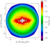 |
Fig. 12 Two-dimensional cut in the (kr, kθ) plane at kφ = 0 through the 3D spectrum of the total kinetic energy in run EX. The dotted white line denotes the disc scale height. |
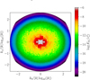 |
Fig. 13 Two-dimensional cut in the (kθ, kφ) plane at kr = 0 through the 3D spectrum of the total kinetic energy in run EX. The dotted white line denotes the disc scale height. This cut is representative of the isotropy observed for kr ≠ 0 and is not a peculiarity of the kr = 0 plane. |
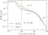 |
Fig. 14 Power spectrum of kinetic energy along k|and k⊥ and power laws expected for critically balanced rotating turbulence, assuming k⊥ = kr and |

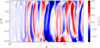 |
Fig. 15 Snapshot of φ-averaged vertical velocity (vz) in run HX at t = 900 orbits. |
3.8 Impact of small-scale turbulence on the large scales
A key question regarding the VSI concerns how the instability saturates. Previous studies propose that parametric instabilities could play a role (Cui & Latter 2022), while Rossby Wave instabilities (Richard et al. 2016) or Kelvin-Helmholtz instabilities (Latter & Papaloizou 2018) could also contribute. An useful element in this discussion is the comparison of vz structures between the cut in the (R, z) plane (Fig. 4, second panel) and the φ-averaged flow taken at the same time (Fig. 15). The φ-averaged flow recovers the large-scale corrugation modes but is much smoother than the φ=0 cut; the small-scale fluctuations visible in Fig. 4 disappear, and therefore must have developed some degree of non-axisymmetry. This suggests that the φ-averaged flow could be treated as a ‘viscous’ 2D version of the full 3D model.
Following this idea, we tested the hypothesis that the nonaxisymmetric flow acts as an effective viscosity on the VSIunstable axisymmetric flow. Hence, we looked for correlations between the azimuthally averaged shear rate ∂〈vi〉/∂ xj and the azimuthally averaged stress tensor due to non-axisymmetric fluctuations  , where 〈·〉 denotes a φ-average and
  . To support this hypothesis, Fig. 16 compares the φ−θ shear and stress components, revealing that the largest turbulent stresses occur where the large-scale shear is strongest. This motivated us to look for general correlations of the form
 (6)
where v is a fourth-order tensor describing the ‘turbulent viscosity’ induced by the small scales on the large axisymmetric scales. By construction, vi j k l is symmetric with respect to i and j.
(6)
where v is a fourth-order tensor describing the ‘turbulent viscosity’ induced by the small scales on the large axisymmetric scales. By construction, vi j k l is symmetric with respect to i and j.
To quantify the relation, Fig. 17 (top panel) presents the probability density function (PDF) of the turbulent θ−φ stress versus the mean vertical shear ∂θ vφ computed from six 3D snapshots of run HX at t = 400, 500, 600, 700, 800, and 900 orbits to produce a temporal average of the stress-shear correlation. This PDF recovers the correlation previously observed in Fig. 16. However, a large dispersion is clearly present. A tentative linear fit (dashed line) to the PDF yields an effective viscosity vθ φ θ φ = 8.1 × 10⁻³ cs H. The stress expectation (solid line) suggests a non-linear relation, showing a slightly stronger turbulent stress response for stronger absolute shear, indicative of a larger turbulent viscosity for larger shears, which steepens as the shear increases. A similar stress response is clearly observed in the correlation between the θ−φ stress versus the mean vertical shear ∂r vθ (Fig. 17, bottom panel), where the fluctuation response increases non-linearly with shear.
Employing such a non-linear turbulent viscosity (i.e., one that depends on the shear) could mimic the effect of 3D small-scale turbulence in 2D large-eddy simulations of the VSI. We also note that the correlation between the θ−φ turbulent stress and the ∂r vθ shear is unexpected in the context of ‘standard’ turbulent viscosity, which typically assumes the viscous tensor to be only non-zero for the components vi j i j. This ‘odd viscosity’ produces peculiar behaviours in complex flows (e.g. Fruchart et al. 2023) that are yet to be understood in the context of turbulent protoplanetary discs. Our findings demonstrate that the turbulent stress response is not only non-linear, but also anisotropic and non-diagonal, confirmed by examination of all possible stress-shear correlations (Appendix B). Developing a turbulent closure scheme is beyond the scope of this work, but our results indicate how to design a turbulent-viscosity model for VSI saturation.
These results suggest that VSI saturation occurs mainly in regions of strong mean axisymmetric shear, where the turbulent response is the largest. Since the strongest shear layers are found at 2-3 scale heights (Fig. 16, top), this indicates that saturation (and therefore energy deposition) probably occurs in the disc atmosphere, rather than in the disc midplane, as a naive α-disc model would suggest.
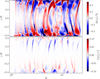 |
Fig. 16 Illustration of the correlation observed between the axisymmetric shear, ∂〈vφ〉/∂ θ (top), and the non-axisymmetric stress tensor, 〈δ vθ δ vφ〉 (bottom), motivating a turbulent viscosity approach. |
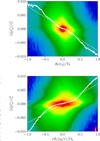 |
Fig. 17 Probability density function (PDF) of the θ−φ (top) and r−θ (bottom) components of shear versus the θ−φ component of the turbulent stress tensor. The turbulent stress expectation for a given shear rate is over-plotted as a solid white line, and the dashed line shows the linear regression of the PDF with turbulent viscosities vθ φ θ φ = 8.1 × 10⁻³ cs H (top) and vθ d r θ = −7.1 × 10⁻³ cs H (bottom). |
4 Conclusions
In this study, we present a detailed numerical investigation of the vertical shear instability (VSI) in locally isothermal protoplanetary discs, focusing on its nonlinear saturation, wave dynamics, and turbulence in 3D. We designed the simulations to capture several large-scale wave zones and a significant portion of the turbulent cascade below the disc scale height (H). Our key findings are summarised below.
First, we find that bulk properties, such as angular momentum flux and kinetic energy density, converge with increasing resolution, with as few as 50 grid points per H sufficient to capture the essential VSI-driven transport. This provides a useful benchmark for future large-scale simulations that aim to include VSI physics at moderate computational cost.
Second, we observe a systematic radial increase in VSI-induced turbulence and transport efficiencies within an extended inner disc region spanning over 20 H, beyond which a true self-similar regime is reached. This trend appears to be artificial, likely stemming from the imposed inner radial boundary conditions, and is consistent with boundary-driven wave-excitation mechanisms discussed in Ogilvie et al. (2025). Caution is therefore warranted when interpreting radial profiles near domain boundaries or in simulations that are not sufficiently radially extended; a minimum of rout/rin ≳ 5 appears necessary to reach an asymptotic regime.
Unlike some previous studies, we do not detect long-lived zonal flows or coherent vortices in our models. This absence may be attributable to our use of a strictly locally isothermal equation of state, which tends to make the VSI more vigorous, or, alternatively, due to our higher resolutions, which might better describe the parametric instabilities that destroy vortices. Finite cooling timescales may be necessary to sustain coherent vortex structures, and further exploration of thermodynamic modelling is needed.
The corrugation-wave phenomenology described by Svanberg et al. (2022) persists in our 3D simulations: the dominant inertial wave frequencies are consistent with those observed in 2D, low-resolution models. However, the 3D wave fields are significantly noisier and the mechanism responsible for this frequency selection remains unclear, warranting further theoretical investigation.
The resulting turbulence exhibits strong anisotropy at large scales, consistent with the phenomenology of critically balanced rotating turbulence. At small scales, the turbulent power spectrum exhibits a distinct break with a very steep power law, echoing the findings ofManger & Klahr (2018), and reflecting numerical viscosity.
Finally, we find that small-scale, non-axisymmetric VSI structures act as an anisotropic effective viscosity on the axisymmetric component of the flow. This emergent behaviour suggests the possibility of developing axisymmetric effective models in which full 3D turbulence is incorporated via a closure scheme, potentially reducing computational costs while retaining key physical effects.
Together, these findings contribute to a growing understanding of VSI dynamics and lay the groundwork for more physically comprehensive and computationally efficient models of protoplanetary disc evolution.
Acknowledgements
We thank Mario Flock, Wladimir Lyra, Orkan Umurhan and Oliver Gressel for useful feedback on the manuscript. The authors acknowledge the EuroHPC Joint Undertaking for awarding this project access to the EuroHPC supercomputer LUMI, hosted by CSC (Finland) and the LUMI consortium through a EuroHPC Extreme Scale Access call. G.L. acknowledges support from the European Research Council (ERC) under the European Union Horizon 2020 research and innovation program (Grant agreement No. 815559 (MHDiscs)). H.L. and G.I.O. are supported by the Science and Technology Facilities Council (STFC) through grant ST/X001113/1.
References
- Barker, A. J., & Latter, H. N., 2015, MNRAS, 450, 21 [NASA ADS] [CrossRef] [Google Scholar]
- Čada, M., & Torrilhon, M., 2009, J. Comput. Phys., 228, 4118 [Google Scholar]
- Cui, C., & Bai, X.-N., 2020, ApJ, 891, 30 [NASA ADS] [CrossRef] [Google Scholar]
- Cui, C., & Bai, X.-N., 2022, MNRAS, 516, 4660 [NASA ADS] [CrossRef] [Google Scholar]
- Cui, C., & Latter, H. N., 2022, MNRAS, 512, 1639 [NASA ADS] [CrossRef] [Google Scholar]
- Dullemond, C. P., Ziampras, A., Ostertag, D., & Dominik, C., 2022, A&A, 668, A105 [NASA ADS] [CrossRef] [EDP Sciences] [Google Scholar]
- Flock, M., Nelson, R. P., Turner, N. J., et al. 2017, ApJ, 850, 131 [Google Scholar]
- Flores-Rivera, L., Flock, M., & Nakatani, R., 2020, A&A, 644, A50 [NASA ADS] [CrossRef] [EDP Sciences] [Google Scholar]
- Fricke, K., 1968, Z. Astrophys., 68, 317 [NASA ADS] [Google Scholar]
- Fruchart, M., Scheibner, C., & Vitelli, V., 2023, Ann. Rev. Condensed Matter Physics, 14, 471 [Google Scholar]
- Goldreich, P., & Schubert, G., 1967, ApJ, 150, 571 [Google Scholar]
- Goldreich, P., & Sridhar, S., 1995, ApJ, 438, 763 [Google Scholar]
- Huang, P., & Bai, X.-N., 2025a, arXiv e-print [arXiv:2503.11076] [Google Scholar]
- Huang, P., & Bai, X.-N. 2025b, ApJ, 986, 1 [Google Scholar]
- Kolmogorov, A., 1941, Doklady Akademiia Nauk SSSR, 30, 301 [Google Scholar]
- Latter, H. N., & Kunz, M. W., 2022, MNRAS, 511, 1182 [CrossRef] [Google Scholar]
- Latter, H. N., & Papaloizou, J., 2018, MNRAS, 474, 3110 [NASA ADS] [CrossRef] [Google Scholar]
- Lesur, G., & Papaloizou, J. C. B., 2009, A&A, 498, 1 [NASA ADS] [CrossRef] [EDP Sciences] [Google Scholar]
- Lesur, G. R. J., Baghdadi, S., Wafflard-Fernandez, G., et al. 2023, A&A, 677, A9 [NASA ADS] [CrossRef] [EDP Sciences] [Google Scholar]
- Lin, M.-K., & Youdin, A. N., 2015, ApJ, 811, 17 [NASA ADS] [CrossRef] [Google Scholar]
- Lovelace, R. V. E., Li, L. H., Colgate, S. A., & Nelson, A. F., 1999, ApJ, 513, 805 [NASA ADS] [CrossRef] [Google Scholar]
- Lubow, S. H., & Pringle, J. E., 1993, ApJ, 409, 360 [Google Scholar]
- Manger, N., & Klahr, H., 2018, MNRAS, 480, 2125 [NASA ADS] [CrossRef] [Google Scholar]
- Manger, N., Klahr, H., Kley, W., & Flock, M., 2020, MNRAS, 499, 1841 [NASA ADS] [CrossRef] [Google Scholar]
- Melon Fuksman, J. D., Flock, M., & Klahr, H. 2024a, A&A, 682, A139 [NASA ADS] [CrossRef] [EDP Sciences] [Google Scholar]
- Melon Fuksman, J. D., Flock, M., & Klahr, H. 2024b, A&A, 682, A140 [NASA ADS] [CrossRef] [EDP Sciences] [Google Scholar]
- Mignone, A., Flock, M., Stute, M., Kolb, S. M., & Muscianisi, G., 2012, A&A, 545, 152 [Google Scholar]
- Nazarenko, S., 2011, Wave Turbulence by Sergey Nazarenko (Berlin: Springer), 825 [Google Scholar]
- Nazarenko, S. V., & Schekochihin, A. A., 2011, J. Fluid Mech., 677, 134 [Google Scholar]
- Nelson, R. P., Gressel, O., & Umurhan, O. M., 2013, MNRAS, 435, 2610 [Google Scholar]
- Ogilvie, G. I., Latter, H. N., & Lesur, G., 2025, MNRAS, 537, 3349 [Google Scholar]
- Pfeil, T., & Klahr, H., 2021, ApJ, 915, 130 [NASA ADS] [CrossRef] [Google Scholar]
- Pfeil, T., Birnstiel, T., & Klahr, H., 2023, ApJ, 959, 121 [NASA ADS] [CrossRef] [Google Scholar]
- Richard, S., Nelson, R. P., & Umurhan, O. M., 2016, MNRAS, 456, 3571 [NASA ADS] [CrossRef] [Google Scholar]
- Shariff, K., & Umurhan, O. M., 2024, ApJ, 977, 26 [Google Scholar]
- Stoll, M. H. R., & Kley, W., 2014, A&A, 572, A77 [NASA ADS] [CrossRef] [EDP Sciences] [Google Scholar]
- Svanberg, E., Cui, C., & Latter, H. N., 2022, MNRAS, 514, 4581 [NASA ADS] [CrossRef] [Google Scholar]
- Urpin, V., & Brandenburg, A., 1998, MNRAS, 294, 399 [Google Scholar]
- Weidenschilling, S. J., 1977, MNRAS, 180, 57 [Google Scholar]
- Zhang, S., Zhu, Z., & Jiang, Y.-F., 2024, ApJ, 968, 29 [Google Scholar]
Appendix A Full 2D kinetic energy spectra
We show in Fig. A.1 the full information on the 2D spectra for each component of the velocity field.
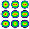 |
Fig. A.1 2D cuts of the kinetic energy spectrum in run EX for each velocity component. The white dotted line delimits the wavenumbers |k|=2 π/H. |
Appendix B Additional shear-stress correlations
We present here additional correlations between the large-scale shear and the turbulent stress from a snapshot from run EX in Fig. B.1. We again find a correlation “by eye” between the large-scale shear and the turbulent stress. We next move to a PDF of all of the possible combinations of stress and shear in Fig. B.2. We observe several correlations that points toward a possible non-diagonal viscous tress tensor. Note however that the large-scale stresses from the axisymmetric corrugation wave are also correlated, so we can’t assert for sure that the viscous stress tensor is non-diagonal from our diagnostics.
Note in addition that for PDFs looking at turbulent stresses versus S = r ∂r〈δ vφ/r〉/ΩK (last line of Fig. B.2), the system never explores the regime S<−0.5. The line S = −0.5 corresponds to marginal Rayleigh stability. We therefore confirm that axisymmetric flows never cross the Rayleigh line.
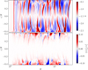 |
Fig. B.1 Illustration of the correlation observed between the axisymmetric shear q (top) and the non-axisymmetric stress tensor 〈δ vr δ vφ〉 (bottom). Note that our large-scale shear includes the mean Keplerian shear which has q = −1.5. |
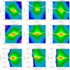 |
Fig. B.2 Probability density function (PDF) of the average shear components versus the turbulent stress tensor components. Overplotted in the solid white line is the turbulent stress expectation for a given shear rate, and in dashed line the linear regression of the PDF that yields the corresponding turbulent viscosity (given in the title of each panel). |
All Tables
Previous studies and their models’ key properties, including the number of dimensions D, radial aspect ratio, number of grid points n per disc scale height H and azimuthal extent Δ φ.
All Figures
|
Fig. 1 Three-dimensional rendering of the meridional velocity sonic Mach number vθ/cs in simulation EX (200 points per H) at t = 800 orbits after restart. The front part shows the flow in the midplane, while the back part shows the flow at 3 H above the midplane, with numerical boundaries at 4 H. The domain has been truncated at Rout = 5.6 to remove the outer wave-killing zone. |
| In the text | |
|
Fig. 2 Radial angular momentum coefficient (α) and poloidal kinetic energy (ek) measured at R = 4 in run HX (solid line) and run LX (dashed line). For clarity, we show the instantaneous α and the time-averaged α over a window of 20 local orbits, 〈α〉t, 20. Run HX was initialized from the saturated state of LX, which explains the absence of an initial transient in HX. |
| In the text | |
|
Fig. 3 Angular momentum transport and poloidal kinetic energy (ek) averaged over the last 400 orbits of the simulations EX (solid line), HX (dashed line), and LX (dotted line). The predicted amplification and saturation radius for a single linear wave train with frequency ω=0.075 Ω0 and n = 1 from Ogilvie et al. (2025) is shown as a dashed green line (Eq. (5)). |
| In the text | |
|
Fig. 4 Instantaneous (R, z) cut of the HX model at t = 900 orbits. Large-scale n = 1 corrugation modes are evident in vz, reaching sonic velocities (top panel), along with shock fronts propagating radially in the density field (bottom panel). |
| In the text | |
|
Fig. 5 Instantaneous (R, φ) cuts of vertical velocity (vz) and density (ρ) in the HX model at t = 900 orbits. Top: midplane cut of vz. Middle: z = 0.3 R (corresponding to 3 pressure scale heights) cut of vz. Bottom: z = 0.3 R cut of the gas density ρ. |
| In the text | |
|
Fig. 6 Spatio-temporal evolution of the azimuthally averaged midplane δ vφ/vK in run HX. Weak zonal flows are observed, with deviations from Kepler of the order of 1%. The flow remains sub-Keplerian in the mid-plane throughout the run. |
| In the text | |
|
Fig. 7 Spatio-temporal evolution of the mean vertical mass flux averaged over φ and θ in simulation HX. Characteristic wave patterns of large-scale corrugation modes, first identified in 2D simulations, are recovered. |
| In the text | |
|
Fig. 8 Radial wavelength probability distribution of the large-scale vertical corrugation motion versus R in run HX, computed over the entire simulation duration. Over-plotted in red are the expected frequency of n = 1 inertial modes for frequencies ω/Ω0 = 0.075, 0.025, 0.0094, and 0.0041. |
| In the text | |
|
Fig. 9 Temporal spectrum of the large-scale vertical corrugation motion versus R in run HX. The dotted lines show the frequencies of the inertial modes plotted in Fig. 8 (ω/Ω0 = 0.075, 0.025, 0.0094., and 0.0041), and the solid line indicates the Keplerian frequency ω=ΩK. |
| In the text | |
|
Fig. 10 Snapshot of the vertical vorticity perturbation in simulation EX at t = 800 orbits in the disc midplane, zooming in of the region around R = 4.5. The image illustrates the complex turbulent flow and the absence of any large-scale coherent vortical structures. |
| In the text | |
|
Fig. 11 Power spectrum of kinetic energy obtained by integrating the 3D spectrum over spherical shells for each velocity field component at the middle of the computational domain in run EX (see text). |
| In the text | |
|
Fig. 12 Two-dimensional cut in the (kr, kθ) plane at kφ = 0 through the 3D spectrum of the total kinetic energy in run EX. The dotted white line denotes the disc scale height. |
| In the text | |
|
Fig. 13 Two-dimensional cut in the (kθ, kφ) plane at kr = 0 through the 3D spectrum of the total kinetic energy in run EX. The dotted white line denotes the disc scale height. This cut is representative of the isotropy observed for kr ≠ 0 and is not a peculiarity of the kr = 0 plane. |
| In the text | |
|
Fig. 14 Power spectrum of kinetic energy along k|and k⊥ and power laws expected for critically balanced rotating turbulence, assuming k⊥ = kr and |
| In the text | |
|
Fig. 15 Snapshot of φ-averaged vertical velocity (vz) in run HX at t = 900 orbits. |
| In the text | |
|
Fig. 16 Illustration of the correlation observed between the axisymmetric shear, ∂〈vφ〉/∂ θ (top), and the non-axisymmetric stress tensor, 〈δ vθ δ vφ〉 (bottom), motivating a turbulent viscosity approach. |
| In the text | |
|
Fig. 17 Probability density function (PDF) of the θ−φ (top) and r−θ (bottom) components of shear versus the θ−φ component of the turbulent stress tensor. The turbulent stress expectation for a given shear rate is over-plotted as a solid white line, and the dashed line shows the linear regression of the PDF with turbulent viscosities vθ φ θ φ = 8.1 × 10⁻³ cs H (top) and vθ d r θ = −7.1 × 10⁻³ cs H (bottom). |
| In the text | |
|
Fig. A.1 2D cuts of the kinetic energy spectrum in run EX for each velocity component. The white dotted line delimits the wavenumbers |k|=2 π/H. |
| In the text | |
|
Fig. B.1 Illustration of the correlation observed between the axisymmetric shear q (top) and the non-axisymmetric stress tensor 〈δ vr δ vφ〉 (bottom). Note that our large-scale shear includes the mean Keplerian shear which has q = −1.5. |
| In the text | |
|
Fig. B.2 Probability density function (PDF) of the average shear components versus the turbulent stress tensor components. Overplotted in the solid white line is the turbulent stress expectation for a given shear rate, and in dashed line the linear regression of the PDF that yields the corresponding turbulent viscosity (given in the title of each panel). |
| In the text | |
Current usage metrics show cumulative count of Article Views (full-text article views including HTML views, PDF and ePub downloads, according to the available data) and Abstracts Views on Vision4Press platform.
Data correspond to usage on the plateform after 2015. The current usage metrics is available 48-96 hours after online publication and is updated daily on week days.
Initial download of the metrics may take a while.