| Issue |
A&A
Volume 703, November 2025
|
|
|---|---|---|
| Article Number | A278 | |
| Number of page(s) | 10 | |
| Section | Galactic structure, stellar clusters and populations | |
| DOI | https://doi.org/10.1051/0004-6361/202556084 | |
| Published online | 24 November 2025 | |
CAPOS: The bulge Cluster APOgee Survey
IX. Spectroscopic analysis of the bulge globular cluster Terzan 2
1
Departamento de Astronomía, Casilla 160-C, Universidad de Concepción,
Concepción,
Chile
2
Universidad Andres Bello, Facultad de Ciencias Exactas, Departamento de Física y Astronomía - Instituto de Astrofísica,
Autopista Concepción-Talcahuano 7100,
Talcahuano,
Chile
3
Departamento de Astronomía, Facultad de Ciencias, Universidad de La Serena,
Av. Juan Cisternas 1200,
La Serena,
Chile
4
Universidad Católica del Norte, Núcleo UCN en Arqueología Galáctica – Inst. de Astronomía,
Av. Angamos 0610,
Antofagasta,
Chile
★ Corresponding author: This email address is being protected from spambots. You need JavaScript enabled to view it.
Received:
24
June
2025
Accepted:
28
August
2025
Abstract
We present the first detailed spectroscopic analysis of the heavily extincted bulge globular cluster Terzan 2 (Ter 2) based on high-resolution near-infrared spectra obtained as part of the CAPOS (bulge Cluster APOgee Survey) project. CAPOS focuses on surveying clusters within the Galactic bulge, using the APOGEE-2S spectrograph, part of the SDSS-IV survey, a component of the second-generation Apache Point Observatory Galactic Evolution Experiment (APOGEE-2). For the spectral analysis, we used the Brussels Automatic Code for Characterizing High accUracy Spectra (BACCHUS) code, which provides line-by-line elemental abundances. We derived abundances for the Fe-peak (Fe, Ni), α (O, Mg, Si, Ca, Ti), light (C, N), odd-Z (Al), and s-process element (Ce) for four members of the cluster. Our analysis yields a mean metallicity of [Fe/H] = −0.84 ± 0.04, with no evidence of intrinsic variation. We detect significant abundance variation only in C and N, indicating the presence of multiple populations. Ter 2 exhibits typical α enrichment, which follows the trend of Galactic globular clusters. Additionally, our dynamical analysis reveals that Terzan 2 is a bulge globular cluster with a chaotic orbit that is influenced by the Galactic bar but not trapped by it, displaying both prograde and retrograde motions within the inner bulge region. Overall, the chemical patterns observed in Terzan 2 are in good agreement with those of other CAPOS bulge clusters of a similar metallicity.
Key words: surveys / stars: abundances / Galaxy: bulge / globular clusters: general / globular clusters: individual: Terzan 2
© The Authors 2025
 Open Access article, published by EDP Sciences, under the terms of the Creative Commons Attribution License (https://creativecommons.org/licenses/by/4.0), which permits unrestricted use, distribution, and reproduction in any medium, provided the original work is properly cited.
This article is published in open access under the Subscribe to Open model. This email address is being protected from spambots. You need JavaScript enabled to view it. to support open access publication.
1 Introduction
Globular clusters (GCs) located in the bulge of the Milky Way are thought to be relics of the early epoch of formation and evolution of the oldest structure in the Galaxy (Bica et al. 2016; Barbuy et al. 2018; Pérez-Villegas et al. 2020). Despite this, bulge GCs (BGCs) have been poorly studied so far (Recio-Blanco et al. 2017; Fernández-Trincado et al. 2019). This is due to the large amount of dust in the Galactic plane and toward the bulge, which generates a high and often variable extinction, making optical observations of these objects difficult (Nataf et al. 2019). In addition, all major components of the Galaxy – the bulge, thin and thick disks, and the halo – reach their highest densities in the inner Galaxy, making both crowding as well as contamination serious problems in areas where extinction is less of an issue.
On the other hand, our understanding of the formation and evolution of GCs has changed dramatically since observations have found the presence of multiple populations (MPs) in them, via the identification of star-to-star variations in the light (C,N), odd-Z (Na, Al), α (O, Mg), and s elements (Fernández-Trincado et al. 2021a). These internal variations demonstrate the complex enrichment in which GCs must have formed. This also provides clues into the conditions of the early Universe in which these systems formed (Renzini et al. 2015). The presence of MPs implies an initial population of stars formed from gas enriched by Type II supernovae, and thus with an overabundance of alpha elements, and a second population of stars presumably formed subsequently from the remaining gas polluted by massive stars of the first population, as is reflected in the C−N, Na−O, and Mg−Al anticorrelations (Smith 1987; Mészáros et al. 2015; Carretta et al. 2009). However, the nature of the first-population polluters (e.g., fast-rotating massive stars, massive binaries, supermassive stars, and/or intermediate-mass AGB stars) and the exact mechanism of the formation of the second population remain unknown (Bastian & Lardo 2018). Further observations are demanded to help constrain various scenarios.
The problem of high extinction is largely minimized with the use of near-infrared (NIR) photometry and high-resolution spectroscopy, which make it possible to penetrate the obscuring dust. In this way, detailed mapping of the chemical and kinematic properties of heavily optically extincted GCs has been possible. In this context, the Apache Point Observatory Galactic Evolution Experiment (APOGEE, Majewski et al. 2017) of the Sloan Digital Sky Survey-IV provided the first high-resolution (R~22 500) near-IR (H-band) multiobject spectrograph in the south. An obvious target is the large sample of BGCs. However, the SDSS-IV APOGEE survey did not prioritize such objects, despite the rather large sample of fields covered in the bulge. Recognizing this opportunity, CAPOS (the bulge Cluster APOgee Survey) was undertaken as a contributing program to SDSS-IV Geisler et al. (2021). A major goal was to obtain high-resolution spectra for a number of members in each of a number of BGCs in order to study their basic chemistry via mean abundances. In addition, CAPOS opened up the study of metal-rich GCs in order to expand the parameter space to explore MPs, since the most metal-rich GCs are only found in the bulge or disk (Bica et al. 2024, Geisler et al. 2025). CAPOS also benefits from the high-precision astrometric and photometric data from the latest release of the ESA Gaia mission (Gaia DR3, Gaia Collaboration 2023), combined with the photometric depth of the Two-Micron All Sky Survey (Skrutskie et al. 2006) and the infrared VISTA Variables in the Vía Láctea (VVV, Minniti et al. 2010; Saito et al. 2012) survey. In the end, CAPOS observed a total of 18 GCs located toward the bulge. An overview of CAPOS and initial results for a subsample are presented in Geisler et al. (2021), based on the APOGEE Stellar Parameters and Chemical Abundance Pipeline (ASPCAP, (García Pérez et al. 2016)) incorporated in SDSS-IV. A second study, focused on FSR 1758, was published by Romero-Colmenares et al. (2021). The third work corresponds to the first high-resolution spectroscopic analysis of Ton 2 (Fernández-Trincado et al. 2022b). Subsequent studies include ones on NGC 6558 (González-Díaz et al. 2023), HP 1 (Henao et al. 2025), NGC 6569 (Barrera et al. 2025) NGC 6316 Frelijj et al. (2025), and the chemical composition of Dorj 2 (Pino et al. 2025). All of these latter studies focus on a single cluster and employ the BACCHUS package (Brussels Automatic Code for Characterizing accUracy Spectra; Masseron et al. (2016). Most recently, Geisler et al. (2025) present final results based on ASPCAP for all CAPOS GCs. This paper is the tenth in the CAPOS series.
The object of this study, which we can see in Figure 1, was first cataloged as Terzan 2. It is a GC located toward the bulge, with l= 356.3 and b=2.30. It has a very high reddening, estimated by Harris (2010) as E(B-V)=1.87. It has been the subject of multiple studies aimed at constraining its fundamental parameters, particularly its metallicity. Early measurements based on integrated infrared photometry estimated [Fe/H] ≈ −0.47 (Malkan & Sargent 1982), while a later study suggested a slightly higher metallicity of [Fe/H] ≈ −0.25 from integrated spectroscopy and infrared color-magnitude diagrams (Kuchinski & Frogel 1995). Terzan 2 is a globular cluster located in the bulge of the Milky Way. It is characterized by an intermediate metallicity for a BGC, with a recently reported value of [Fe/H] = −0.85 (Geisler et al. 2021; Harris 2010) gave −0.69.
According to Baumgardt & Vasiliev (2021) the cluster has a mass of 8.05 ± 2.31 ⋅ 104 M⊙, a distance from the Sun of 7.75 ± 0.33 kpc, a galactocentric distance of 0.74 ± 0.16 kpc, and a tidal radius of 12.45 pc. This BGC is an important object for studying the chemical and dynamical evolution of the inner regions of our galaxy, offering insights into the complex formation history of the bulge and its stellar populations.
CAPOS data provide a spectroscopic metallicity more robust than any current available for Terzan 2, as well as detailed abundances for many elements with a wide variety of nucleosynthetic origins, including the α (0, Mg, Si, Ca, Ti), Fe-peak (Fe, Ni), light (C, N), odd-Z (Al), and s-process (Ce) elements. The chemical abundances of Terzan 2 were derived using the BACCHUS package (Brussels Automatic Code for Characterizing accUracy Spectra; Masseron et al. 2016). A rigorous line-by-line inspection was performed across spectra encompassing a range of abundance variations, allowing for the determination of optimal fit values for each element with maximal reliability.
This paper is organized as follows. Section 2 describes the spectroscopic data used. In Section 3, we review the target selection. Section 4 shows the parameter selection. In Section 5, we present the abundance determinations. The results are described in Section 6. A dynamical analysis of the cluster is present in Section 7. Finally, we present our summary and concluding remarks in Section 8.
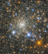 |
Fig. 1 Bulge globular cluster Terzan 2 captured by the Hubble Space Telescope. Credit: NASA, ESA, ESA/Hubble, Roger Cohen (RU). |
2 Spectroscopic data
The analysis was carried out on high-resolution (R≈22 500) NIR spectra obtained by the Apache Point Observatory Galactic Evolution Experiment II survey (APOGEE-2; Majewski et al. (2017)), an internal program of SDSS-IV (Blanton et al. 2017), with the aim of delivering accurate radial velocities and detailed chemical abundances for a large sample of giant stars covering all components of the Milky Way and nearby dwarf companions.
The APOGEE-2 survey uses two spectrographs (Wilson et al. 2019): one from the northern hemisphere on the 2.5 m telescope at Apache Point Observatory (APO, APOGEE-2N; Gunn et al. (2006)) and another from the southern hemisphere on the Irénée du Pont 2.5 m telescope (Bowen & Vaughan 1973) at Las Campanas Observatory (LCO, APOGEE-2S). Each instrument records most of the H band (1.5–1.69 µm) on three detectors, with coverage gaps between ~ 1.58–1.59 µm and ~ 1.64–1.65 µm, and with each fiber subtending 2″ in diameter on the sky in the northern instrument and 1.3″ in the southern.
The final release of APOGEE-2, Data Release 17 (DR17), from SDSS-III/SDSS-IV, includes all data collected at APO through November 2020 and at LCO through January 2021, with the two APOGEE-2 instruments having observed over 650 000 stars across the Milky Way. Target selection is detailed in Zasowski et al. (2017), Beaton et al. (2021), and Santana et al. (2021). Spectra were reduced as described in Nidever et al. (2015), and analyzed using the APOGEE Stellar Parameters and Chemical Abundance Pipeline (ASPCAP; García Pérez et al. (2016)), and the libraries of synthetic spectra described in Zamora et al. (2015). The customized H-band line lists are fully described in Shetrone et al. (2015), Hasselquist et al. (2016) (neodymium lines (Nd II)), Cunha et al. (2017) (cerium lines (Ce II)), and Smith et al. (2021). CAPOS was a Contributed APOGEE program (Geisler PI) allocated by the CNTAC designed to study as large a sample of BGCs. Most recently, Geisler et al. (2025) have presented final ASPCAP-based abundances for the entire 18 cluster CAPOS sample. Terzan 2 was observed as part of the contributing CAPOS survey (Geisler et al. 2021).
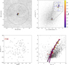 |
Fig. 2 Membership selection of Terzan 2 targets. Top panels (left): spatial position. Star symbols correspond to the selected targets and are color-coded by the S/N of the APOGEE spectra (as is labeled in the color bar in the top right panel; all panels share the same color scale). Other APOGEE targets in the field are gray dots. A circle with the tidal radius 9.49′ (Harris 2010) is overplotted. (right) Proper motion density distribution of stars located within the tidal radius from the cluster center, color- and size-coded as in the top left panel. The inner plot on the top right shows a zoom-in of the cluster in 0.7 × 0.7 mas yr−1 and enclosed in a PM radius of 0.5 mas yr−1 shown in a blue circle. Dashed blue lines are centered on the cluster center PM values (Baumgardt & Vasiliev 2021). Bottom panels (left): radial velocity from ASPCAP vs. metallicity of our members compared to field stars. The [Fe/H] of our targets have been determined with BACCHUS (see Sect. 4), while the [Fe/H] of field stars (gray dots) are taken from the ASPCAP pipeline. The astrometric, photometric, and kinematic parameters used are listed in Table 1. The red box encloses the cluster members within 0.1 dex and 10 km/s from the nominal mean [Fe/H]=−0.84 and RV=10.2 km s−1 of Terzan 2, as determined in this work. (right) CMD corrected by differential reddening and extinction-corrected in the Gaia Bp band and 2MASS K band of our sample and using stars within 9.49′. Our targets all lie along the RGB. The best isochrone fit (purple circles), corresponding to [M/H]= −0.80 is overplotted on Terzan 2 stars (red dots) located within 9.49 arcminutes of the cluster center and has been shifted using E(B−V)=2.081, Aυ=5.16, and Rυ=2.48. |
3 Target selection
The APOGEE-2S plug-plate containing Ter 2 (toward αJ2000 = 17h27m33.1s and δJ2000 = −30d48m08.4s) was centered on (l, b) ~ (356.3°, 2.30°) inside a radius of ≤15′ from the cluster center. The Gaia database was not available at the time of the observations, so we based our selection on existing CMDs and selecting targets within the tidal radius of the cluster (Harris 2010, 9.49′) to find the most likely members, as is shown in Figure 2 (Top panels (left)) and described in Geisler et al. (2021).
After observations were obtained, we began our search to maximize membership. The procedure is described in detail in Geisler et al. (2025). Basically, we first limited our sample to observed stars within the tidal radius of the cluster Baumgardt & Vasiliev (2021). We later matched this initial spatially selected sample with the released Gaia DR2 (Gaia Collaboration 2018) catalog and required proper motions (PMs) within a radius of 0.5 mas yr−1 around the mean PM of Ter 2: µα cos(δ) = −2.13 and µδ = −6.34 (Baumgardt & Vasiliev 2021). We initially used these values to estimate candidate members from the PMs and to reduce the potential field star contamination in the optical and NIR color-magnitude diagrams (CMDs). We later reexamined PM from the original sample using the data from the Gaia DR3 data release (Gaia Collaboration 2023). Figure 2 (Top panels (right)) shows the PMs using Gaia DR3 (Gaia Collaboration 2023).
Figure 2 (Bottom panels (left)) also shows the BACCHUS [Fe/H] abundance ratios (see Section 6) versus the radial velocity of our four cluster members compared to field stars with ASPCAP/APOGEE-2 [Fe/H] determinations, which were shifted by +0.11 dex in order to minimize the systematic differences between ASPCAP/APOGEE-2 and BACCHUS, as is highlighted in Appendix D of Fernández-Trincado et al. (2020a). We note that all of our targets have very similar velocities that are extreme compared to the field star distribution. This again supports the cluster membership for all of our targets.
We find a mean RV from four APOGEE-2 stars of 133.4±1.46 km s−1, which is in very good agreement with the value listed in Baumgardt’s web service1, RV= 133.46 ± 0.69 km s−1. The red box highlighted in this plot encloses the cluster members within a box centered on the mean [Fe/H]=−0.84 and RV=133.4 km/s of Ter 2. After this, we were left with four very high-probability members. We checked that all of them are positioned along the red giant branch (RGB) of the cluster, as is shown in the differential reddening-corrected CMD (see Figure 2 (Bottom panels (right))).
All selected stars had 2MASS K-band magnitudes brighter than 13. This was required in order to achieve a minimum signal-to-noise ratio (S/N) of >60 pixel−1 in one plug-plate visit (~1 hour). The four stars observed have S/N > 100 pixel−1, since more than one visit was obtained. Table 1 lists the APOGEE-2S designations of the stars, the APOGEE-2S coordinates, S/N, Gaia DR3 and 2MASS magnitudes, RV, and PMs.
APOGEE and Gaia DR3 data for Terzan 2 candidate stars.
4 Atmospheric parameters
The CMD presented in Figure 2 (Bottom panels (right)) was differential-reddening-corrected using the same methodology as was employed in Romero-Colmenares et al. (2021) and Fernández-Trincado et al. (2022b). For this purpose, we selected all RGB stars within a radius of 3.5 arcmin from the cluster center and that have PMs compatible with that of Ter 2. First, we drew a ridge line along the RGB, and for each of the selected RGB stars we calculated its distance from this line along the reddening vector. The vertical projection of this distance gives the differential interstellar absorption, AK, at the position of the star, while the horizontal position gives the differential optical+NIR reddening E(BP−K) at the position of the star. After this first step, for each star we selected the three nearest RGB members, calculated the mean differential interstellar absorption, AK, and the mean differential reddening, E(BP−K), and finally subtracted these mean values from its BP−K color and K magnitude. We underline the fact that the number of reference stars used for the reddening correction is a compromise between having a correction affected as little as possible by random photometric errors and the highest possible spatial resolution.
In order to estimate the parameters of the cluster, we performed isochrone fitting of the RGB using the PARSEC database (Bressan et al. 2012). The extinction law of Cardelli et al. (1989) and O’Donnell (1994) was used. The free parameters for this fitting are the true distance modulus, (m − M)0 (or the equivalent distance in parsecs), the interstellar absorption in the V band, AV, and the reddening-law coefficient, RV. These three parameters were estimated simultaneously using the BP−K versus K, BP−RP versus G, and J−K versus K CMDs, assuming an age of 12 Gyr and initially a global metallicity of [M/H]=−0.8 that considers the α enhancement of the cluster according to the relation by Salaris et al. (1993). [Fe/H] was obtained from Harris (2010) and [α/Fe] assumed to be +0.4. [M/H] was then adjusted during the fitting procedure in order to match the shape of the upper RGB.
The coefficient of the extinction law, RV, is usually assumed to be 3.1 but can vary significantly from the canonical value, especially in the direction of the Galactic bulge (Nataf et al. 2016), where it can easily take lower values. In fact, we find an extinction law coefficient RV = 2.48 ± 0.1. Moreover, we achieve a fit for the distance of d⊙ = 9.8 kpc, i.e., (m − M)0=14.95 ± 0.05, higher than previous estimations such as 7.75±0.33 kpc from Baumgardt & Vasiliev (2021) or 7.5 kpc from Harris (2010), and an interstellar absorption of AV = 5.16 ± 0.05. Finally, the interstellar absorption and the extinction-law coefficient we found can be translated into E(B-V)= 2.08, which is somewhat higher than the foreground interstellar reddening given by Harris (2010), i.e., E(B-V)=1.87. This discrepancy is very likely due to the higher RV used in previous studies.
The method applied to obtain Teff and log 𝑔 from photometry was the same as the one described in Fernández-Trincado et al. (2022b). We used the differentially corrected BP−K versus K CMD of Figure 2 (Bottom panels (right)) and projected horizontally the position of each target until it intersected the RGB of the best fitting isochrone. We then assumed the Teff and log 𝑔 of each target to be the temperature and gravity of the point of the isochrone that has the same Ks magnitude as the star, interpolating if necessary. We underline the fact that, for highly reddened objects such as Terzan 2, the interstellar absorption correction depends on the spectral energy distribution of the star; that is, on its temperature. For this reason, we applied a temperature-dependent absorption correction to the isochrone. Without this procedure, it is not possible to obtain a proper fit of the RGB, especially of the brighter and cooler part. Finally, with Teƒƒ and log 𝑔 fixed, we employed the relation from Mott et al. (2020) for FGK stars to determine the microturbulence parameter, ξt. The obtained stellar parameters are listed in Table 2.
5 Abundance determination
The method of deriving stellar abundances is the same as that described in Fernández-Trincado et al. (2022b). For this purpose, we made use of the Brussels Automatic Code for Characterizing High accUracy Spectra (BACCHUS) Masseron et al. (2016) to derive chemical abundances for the entire sample, making a careful line selection as well as providing abundances based on a simple line-by-line approach. The BACCHUS module consists of a shell script that computes on the fly synthetic spectra for a range of abundances and compares these spectra to the observational data on a line-by-line basis, deriving abundances from different methods (e.g., using the equivalent width, the line depth, or the χ2). For the synthetic spectra, BACCHUS relies on the radiative transfer code Turbospectrum (Alvarez & Plez 1998; Plez 2012) and the MARCS model atmosphere grid (Gustafsson et al. 2008).
The APOGEE-2 spectra provide access to 26 chemical species, on which we were able to provide reliable abundance determinations for 11 selected chemical species, belonging to the iron-peak (Fe, Ni), odd-Z (Al), light (C,N), α (O, Mg, Si, Ca and Ti), and s-process (Ce) elements. This is due to the fact that most of the atomic and molecular lines are very weak and heavily blended, in some cases too much to produce reliable abundances in cool, relatively metal-poor BGC stars.
As is described in Fernández-Trincado et al. (2022b), we did not include sodium in our analysis, a typical species used to separate GC MPs, as it relies on two atomic lines (Na I: 1.6373 µm and 1.6388 µm) in the H band of the APOGEE-2 spectra, which are generally very weak and heavily blended by telluric features and therefore cannot produce reliable [Na/Fe] abundance determinations in GC with the Teƒƒ and metallicities typical of Ter 2. This is why we focus on the elemental abundances of Al, Mg, C, N, and O, which are the chemical signatures that allow us to distinguish stars with different chemical compositions in the MP phenomenon.
From these synthetic spectra, the BACCHUS code then identified the continuum points for normalizing the observed spectra and the relevant pixels (i.e., a mask or window) to use for the abundance determination of each line in each spectrum. The normalization was performed by selecting continuum regions in the synthetic spectra within 30 Å around the line of interest, and fitting a linear relation to these regions in the observed spectrum. Then the observed spectrum was divided by this fit.
The spectral window for each line was defined by identifying the regions where variations in elemental abundance cause noticeable changes in the synthetic spectra. This was done by analyzing the second derivative of the observed flux to locate the local maxima on either side of the target line.
For each element and spectral line, the abundance determination follows the procedure described in Hawkins et al. (2016), Fernández-Trincado et al. (2021a), Cunha et al. (2017), and Romero-Colmenares et al. (2021); thus, we only provide a brief summary here. The abundance of each chemical species was derived through the following steps: (a) a spectral synthesis was performed using the complete atomic and molecular line list from Shetrone et al. (2015), Hasselquist et al. (2016), and Smith et al. (2021), internally labeled as linelist.20170418 (reflecting the creation date in YYYYMMDD format), which was also used to determine the local continuum level via a linear fit; (b) cosmic ray and telluric contamination were identified and removed; (c) the local S/N was estimated; (d) flux points contributing to each absorption line were automatically selected; and (e) the observed spectrum was compared with a grid of convolved synthetic spectra spanning a range of abundances to determine the best fit. Finally, four different methods were applied to derive the abundances:
Line-profile fitting (the χ2 method), which determines the abundance by minimizing the squared differences between the synthetic and observed spectra. This approach fits the entire line profile, providing a comprehensive evaluation of the spectral match.
Core line-intensity comparison (the int method), which focuses on matching the intensity at the core of the line between the synthetic and observed spectra. This method is particularly effective for analyzing the central features of spectral lines, where the abundance signature is most pronounced.
Global goodness-of-fit estimation (the syn method), which derives the abundance by minimizing the overall discrepancy between the synthetic and observed spectra, assessing the global quality of the fit rather than focusing on specific line features.
Equivalent-width comparison (the eqw method), which estimates the abundance required to reproduce the observed equivalent width of a spectral line. This widely used technique reduces the spectral information to a single value, the area under the line profile, simplifying the comparison process.
Each diagnostic yields validation flags. Based on these flags, a decision tree then rejects or accepts each estimate, keeping the best-fit abundance. We adopted the χ2 diagnostic as the final abundance because it is the most robust (Hawkins et al. 2016). However, we stored the information from the other diagnostics, including the standard deviation among all four methods.
12C, 14N, and 16O elemental abundances were derived through a combination of vibration-rotation lines of 12C16O and 16OH, along with electronic transitions of 12C14N. The procedure for CNO analysis began by setting the C abundance using 12C16O lines. With this carbon abundance, the O abundance was determined using 16OH lines. If this O abundance differed from the initial value, which was scaled from the solar value by the stellar [Fe/H] ratio, the 12C16O lines were reanalyzed with the updated O abundance, until consistent C and O abundances were obtained from both 12C16O and 16OH. When consistent values for C and O were obtained, the12 C14N lines were used to derive the N abundance, which had little to no effect on the 12C16O and 16OH lines, but the final abundances of C, N, and O provided self-consistent results from 12C16O, 16OH, and 12C14N Smith et al. (2013). The molecular dependencies of CNO were extracted from this process.
In order to provide a consistent chemical analysis, we rede-termined the chemical abundances assuming as inputs the effective temperature (Teƒƒ), surface gravity (log 𝑔), and metallicity ([Fe/H]) derived by the ASCAP pipeline (García Pérez et al. 2016). However, we also applied a simple approach of fixing Teƒƒ and log 𝑔 to values determined independently of spectroscopy, in order to check for any significant deviation in chemical abundances and to minimize a number of ca-feats present in ASCAP/APOGEE-2 abundances for GCs (see e.g., Masseron et al. 2019; Mészáros et al. 2020; Romero-Colmenares et al. 2021), as it is affected by a systematic effect that most likely overestimates the Teƒƒ values of 2P stars (Geisler et al. 2021).
The final values of each elemental abundance are summarized in Table 2, where we compare them with the mean values estimated by ASPCAP. We have also compared our results with other BGCs of a similar metallicity, such as M107 from Mészáros et al. (2020) and NGC 6569 from Barrera et al. (2025), as is shown in Figure 3.
The total uncertainty, σtot, was calculated as the square root of the sum of the squares of the individual uncertainties obtained from the errors in each atmospheric parameter and S/N treated independently, according to the following equation:
 (1)
(1)
where each deviation, σ, represents the change in our initial central abundance estimation after running BACCHUS with atmospheric parameters varied by Teƒƒ ± 100 K, log 𝑔 ± 0.3 cgs, and ξt ± 0.05 km/s. These values were chosen as they represent the typical conservative uncertainties in the atmospheric parameters for our sample. This implies running BACCHUS for each of the different atmospheric parameters and statistically measuring the variations. The results of this analysis are reported in Table 3 for the star with the highest S/N in our sample, which consequently exhibits the smallest uncertainties. These uncertainties are comparable to those of the other stars in our sample.
Elemental abundances of Terzan 2 members.
6 Results
6.1 Iron-peak elements (Fe and Ni)
Our analysis yields a mean metallicity of [Fe/H]=−0.84±0.04, with a dispersion of 0.06 dex, which is mainly produced by the relatively high metallicity (−0.74) of the star 2M172731853048156. However, comparing the observed dispersion with the total iron error in Table 2, we find that there is no significant metallicity spread, which confirms that Ter 2 is consistent with other GCs with similar metallicity, as is seen in Figure 3.
It is important to note that our mean metallicity is in very good agreement with ASPCAP DR17, as is shown in Table 2. The value of Harris (2010) [Fe/H] for this cluster is −0.69, based on integrated low-resolution Ca triplet (CaT) spectroscopy (Armandroff & Zinn 1988) and near-IR low-resolution spectra of seven stars (Stephens & Frogel 2004). On the other hand, Geisler et al. (2021) gives an even closer value, [Fe/H]=−0.85±0.04, from their initial ASPCAP analysis. Geisler et al. (2025) find a value of [Fe/H]=−0.88±0.02 from basically the same data but using ASPCAP (but note that ASPCAP abundances are not available for the star 2M17273364-3047243). However, Geisler et al. (2023) derived a significantly higher value of [Fe/H]=−0.54±0.10 from Ca triplet data for eight members.
The metallicity that we find for Terzan 2 places it near the high-metallicity tail of the dominant, metal-poor peak of the BGC metallicity distribution (Geisler et al. 2025). Bulge GCs of comparable metallicities have been poorly studied within a radius of ~4 kpc of the Galactic center. There is little detailed chemical information for some of these (such as Pal 6, Pal 12, and E3). For this reason, in Fig. 3 we compare our chemical abundances obtained for Ter 2 with M107, a BGC taken from Mészáros et al. (2020), and NGC 6569 from Barrera et al. (2025), a BGC from CAPOS that has a similar metallicity to the one of our cluster. In this figure, we do not plot Ti and Ni, both belonging to the iron-peak group, since Mészáros et al. (2020) do not report their abundances.
Nevertheless, nickel (Ni) is included in our analysis and shows an average abundance of 〈[Ni/Fe]=+0.01〉±0.02, with a dispersion of 0.03 dex. This abundance is slightly lower (≲0.04 dex) than the abundance ratios measured by ASPCAP DR17. The abundance ratio [Ni/Fe] in Ter 2 is similar to that observed in objects of a similar metallicity, as is seen in Figure 3.
Typical abundance uncertainties for Terzan 2 target star.
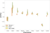 |
Fig. 3 [X/Fe] and [Fe/H] distributions of Terzan 2. [X/Fe] and [Fe/H] abundance density estimation (violin representation) of Terzan 2 (orange), compared to elemental abundances of M107 (green) from Mészáros et al. (2020) and NGC 6569 (yellow) from Barrera et al. (2025). |
6.2 The light elements C and N
We find that Ter 2 exhibits a high enrichment in nitrogen, with a mean abundance of [N/Fe]=+0.81±0.31, with a large dispersion of 0.35 dex, and an average carbon deficiency of [C/Fe]=−0.21±0.15 with a dispersion of 0.16 dex, which is lower than the value [C/Fe]=−0.08 calculated by ASPCAP DR17, while our [N/Fe] value is higher.
Figure 4 shows a clear anticorrelation in C−N as well as N−O. However, there is no sign of a N-Al correlation. The behavior of C and N is comparable to that observed in M107 and NGC 6569. The lack of a N-Al correlation in Ter 2 could be due to our limited sample of targets and future observations are required to verify this finding. Also, measurements indicate that Ter 2 is populated by a fraction of stars with enhanced [N/Fe] abundances well above typical galactic values ([N/Fe]≳+0.5). This is a common behavior for GCs, and a clear indication of multiple stellar populations (see e.g., Schiavon et al. 2017; Fernández-Trincado et al. 2020b; Geisler et al. 2021). Interestingly, one of the analyzed stars, 2M17273540–3047308, shows a rather low [N/Fe] abundance, more consistent with a first stellar population. This contrast further reinforces the presence of a chemical spread in nitrogen and is compatible with the existence of MPs in Terzan 2.
6.3 The α elements: O, Mg, Si, Ca, and Ti
Figure 3 and Table 2 show that Ter 2 exhibits a considerable α-element enhancement, with mean values of: [O/Fe] =+0.28±0.04, [Mg/Fe] = + 0.40±0.04, [Si/Fe] = +0.33±0.06, [Ca/Fe] = +0.28±0.04, and [Ti/Fe] = +0.20±0.06, with no evidence of an intrinsic spread in any of these elements. These values are in good agreement with GCs of a similar metallicity. The α elements in Ter 2 are overabundant compared to the Sun, which is a common behavior in Galactic GCs and field stars at a similar metallicity, such as M107 and NGC 6569. The agreement with ASPCAP DR17 is generally very good, with a difference of 0.02 dex in the worst case (that is, for [Si/Fe]).
Geisler et al. (2025) find the same mean [Si/Fe] from ASP-CAP. They also point out a systematic difference in [Si/Fe] for the CAPOS clusters in general between the BACCHUS and ASP-CAP abundances, with BACCHUS on average 0.17±0.07 dex higher.
6.4 The odd-Z element Al and the s-process element Ce
Ter 2 exhibits a mean aluminum enrichment of [Al/Fe]=+0.24±0.08, with a dispersion of 0.09 dex. We did not find a variation in [Al/Fe] beyond the typical errors. However, if we compare [Al/Fe] to [Mg/Fe] (see Fig. 4), we see that there is a hint of Mg-Al. If real, this means that the Mg-Al cycle barely started in the stars that were responsible for the intracluster contamination. This is consistent with expectations of AGB nucleosynthesis (Fernández-Trincado et al. 2021b; Ventura & D’Antona 2008; García-Hernández et al. 2016; Karakas & Lattanzio 2014).
We find a mean abundance of [Ce/Fe]=+0.11±0.03, which is slightly super-solar, and comparable to the Ce levels observed in other Galactic GCs at a similar metallicity (see e.g., Masseron et al. 2019; Mészáros et al. 2020). The observed spread for the s-process element Ce is +0.03 dex, with no indication of intrinsic dispersion. Figure 4 reveals that there is no correlation between Ce and N. This result does not show the correlation between Ce and N observed by Fernández-Trincado et al. (2022b) in the clusters Ton 2 and Fernández-Trincado et al. (2021a) in NGC 6380, suggesting that the chemical enrichment history of Terzan 2 may differ from that of those clusters. Consistently, the agreement with ASPCAP DR17 is very good for [Ce/Fe] with a difference of 0.04 dex, and slightly worse for [Al/Fe], with a difference of 0.11 dex.
7 Dynamical history
We made use of the state-of-art Milky Way model −GravPot162 to predict the orbital path of Terzan 2 in a steady-state Galactic gravitational model that includes a “boxy peanut” bar structure (Fernández-Trincado et al. 2019). Orbits have been integrated with the GravPot16, which includes the perturbations due to a realistic (as far as possible) rotating “boxy peanut” bar, which fits the structural and dynamical parameters of the Galaxy based on recent knowledge of our Milky Way.
For the orbit computations, we adopted the same model configuration, solar position, and velocity vector as are described in Fernández-Trincado et al. (2019), except for the angular velocity of the bar, Ωbar, for which we employed the recommended value of 41 km s−1 kpc−1 (Sanders et al. 2019) and assuming variations of ± 10 km s−1 kpc−1. The considered structural parameters of our bar model (e.g., mass and orientation) are within observational estimations that lie in the range of 1.1 ×10¹⁰ M⊙ and present-day orientation of 20° (value adopted from dynamical constraints of Tang et al. 2018) in the non-inertial frame (where the bar is at rest). The bar scale lengths are xo=1.46 kpc, yo=0.49 kpc, and zo =0.39 kpc, and the middle region ends at the effective semimajor axis of the bar, Rc=3.28 kpc (Robin et al. 2012).
For guidance, the Galactic convention adopted by this work is: the X axis is oriented toward l=0° and b=0°, the Y axis is oriented toward l=90°, and the velocity is also oriented in these directions. Following this convention, the Sun’s orbital velocity vectors are [U⊙, V⊙, W⊙]=[11.1, 12.24, 7.25] km s−1 (Schönrich et al. 2010). The model has been rescaled to the Sun’s Galactocentric distance, 8.27 kpc (GRAVITY Collaboration 2021), and a circular velocity at the solar position, to be ~229 km s−1 (Eilers et al. 2019). Table 4 gives our input parameters and their errors.
The most likely orbital parameters and their uncertainties were estimated using a simple Monte Carlo scheme. An ensemble of one million orbits was computed backward in time for 2 Gyr, under variations of the observational parameters, assuming a normal distribution for the uncertainties of the input parameters (e.g., positions, heliocentric distances, radial velocities, and PMs), which were propagated as 1σ variations in a Gaussian Monte Carlo resampling. To compute the orbits, we adopted a mean radial velocity from the member stars from APOGEE DR17 data (Abdurro’uf et al. 2022) reported by Baumgardt & Vasiliev (2021). The nominal PMs (〈µRA〉) and 〈µDec〉) for Terzan 2 were taken from Gaia EDR3 (Gaia Collaboration 2021), assuming an uncertainty of 0.5 mas yr−1 for the orbit computations. The heliocentric distance (d⊙) was also adopted from Baumgardt & Vasiliev (2021). The results for the main orbital elements are listed in the inset of Figure 5.
Figure 5 shows the simulated orbital path of Terzan 2 by adopting a simple Monte Carlo approach. The probability densities of the resulting orbits are projected on the equatorial and meridional galactic planes, in the non-inertial reference frame where the bar is at rest. The black line in the figure shows the orbital path (adopting observables without uncertainties). The yellow color corresponds to the most probable regions of the space, which are crossed more frequently by the simulated orbits. Terzan 2 is clearly confined in a bulge-like orbit, which lies in an in-plane orbit with high eccentricity >0.9 and low vertical (Zmax < 0.6 kpc) excursions from the Galactic plane, and apogalactocentric distances below 1 kpc. This cluster is going inside and outside of the bar in the Galactic plane, but not with a bar-shaped orbit, which means that this cluster is not trapped by the bar, but exhibits a chaotic orbital motion that experiences both prograde and retrograde orbits, whose effect is produced by the presence of the bar. From the average orbital parameters listed in Figure 5, we can see that the Galactic bar induced the orbit to have smaller average (peri-/apo-) galactic distances, lower vertical excursions from the Galactic plane, and higher eccentricities, even for any of the bar pattern speed values, suggesting that the presence of different Ωbar in Terzan 2 is almost negligible. The bulge nature of this cluster derived from its orbit here agrees with the classification by Geisler et al. (2025) based on the synthesis of a number of both dynamical and chemical analyses.
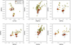 |
Fig. 4 Abundance distributions. From left to right, the top row shows the distributions of [N/Fe]–[C/Fe], [Al/Fe]–[Mg/Fe], and [O/Fe]–[N/Fe]; the bottom row shows [Al/Fe]–[N/Fe], [Al/Fe]–[Si/Fe], and [Ce/Fe]–[N/Fe]. The data correspond to Terzan 2 stars from this work (orange stars), M107 (green circles) from Mészáros et al. (2020), and NGC 6569 (yellow circles) from Barrera et al. (2025). Typical uncertainties for Terzan 2 stars are also indicated. |
Input parameters adopted for the orbital integration of Terzan 2.
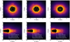 |
Fig. 5 Ensemble of one million orbits for Terzan 2 in the frame corotating with the MW bar, projected on the equatorial (top) and meridional (bottom) Galactic planes in the non-inertial reference frame with a bar pattern speed of 31 (left), 41 (middle) and 51 (right) km s−1 kpc−1, and time-integrated backward over 2 Gyr. The yellow and orange colors correspond to more probable regions of the space, which are most frequently crossed by the simulated orbits. The solid black line shows the orbital path of Terzan 2 from the observables without error bars. |
8 Conclusions
We present the first detailed elemental-abundance analysis for four stars of the BGC Terzan 2, as part of the CAPOS survey using APOGEE-2 data. We examine 11 chemical species: the light elements C and N, the α elements O, Mg, Si, Ca, and Ti, the iron-peak elements Fe and Ni, the odd-Z element Al, and the s-process element Ce using the BACCHUS code. Overall, the chemical species examined so far in Ter 2 are in general agreement with other Galactic GCs at a similar metallicity from Mészáros et al. (2020) and Barrera et al. (2025). The main conclusions of this paper are the following:
The mean metallicity of Terzan 2 is [Fe/H]=−0.84±0.04, with a star-to-star [Fe/H] spread that is not statistically significant, indicating a homogeneous iron content;
Our value of metallicity is lower than the classical value of −0.69 from Harris (2010). It is in good agreement with other ASPCAP studies of the same cluster, in particular −0.88±0.02 from Geisler et al. (2025). However, it is significantly lower than values derived using the CaT technique, such as −0.54±0.10 from Geisler et al. (2023), pointing to the difficulty of obtaining accurate metallicities for such highly obscured GCs and such small samples. It is a member of the dominant lower-metallicity peak of the BGC metallicity distribution;
Even with the low number of stars analyzed, there is an apparent anticorrelation between C-N, a common feature among globular clusters (e.g., Mészáros et al. (2020)). A spread in [N/Fe] has been detected in Terzan 2 (~0.5 dex). This result indicates that Terzan 2 is likely to host the multiple-population phenomenon, but any firm conclusion should await a substantial increase in sample size;
The alpha elements align with the trends commonly observed in globular clusters within the same metallicity range (Mészáros et al. 2020) with an enhancement of between 0.2–0.4 dex;
We do not find evidence of a real spread in Ce abundances in Terzan 2. Furthermore, the apparent Ce-N and Ce-Al correlations reported in other bulge globular clusters (e.g., Ton 1 and Ton 2) at a similar metallicity (see Fernández-Trincado et al. 2021, 2022) are not observed in our data;
Our dynamical analysis suggests that Terzan 2 is a BGC. It lives in the inner bulge region, but goes inside and outside of the bar in the Galactic plane, with a non-bar-shaped orbit, which means that Terzan 2 is not trapped by the bar but exhibits a chaotic orbital motion that describes prograde and retrograde paths at the same time, whose effect is produced by the presence of the bar.
Acknowledgements
Part of this work was supported by the German Deutsche Forschungsgemeinschaft, DFG project number Ts 17/2-1. S.V. gratefully acknowledges the support provided by Fondecyt Regular n. 1220264 and by the ANID BASAL project FB210003. D.G. gratefully acknowledges the support provided by Fondecyt Regular n. 1220264. D.G. also acknowledges financial support from the Dirección de Investigación y Desarrollo de la Universidad de La Serena through the Programa de Incentivo a la Investigación de Académicos (PIA-DIDULS).
References
- Abdurro’uf, Accetta, K., Aerts, C., et al. 2022, ApJS, 259, 35 [NASA ADS] [CrossRef] [Google Scholar]
- Alvarez, R., & Plez, B. 1998, A&A, 330, 1109 [NASA ADS] [Google Scholar]
- Armandroff, T. E., & Zinn, R. 1988, AJ, 96, 92 [Google Scholar]
- Asplund, M., Grevesse, N., & Sauval, A. J. 2005, in Astronomical Society of the Pacific Conference Series, 336, Cosmic Abundances as Records of Stellar Evolution and Nucleosynthesis, eds. T. G. Barnes, III, & F. N. Bash, 25 [NASA ADS] [Google Scholar]
- Barbuy, B., Chiappini, C., & Gerhard, O. 2018, ARA&A, 56, 223 [Google Scholar]
- Barrera, N., Villanova, S., Geisler, D., Fernández-Trincado, J. G., & Muñoz, C. 2025, A&A, 699, A128 [NASA ADS] [CrossRef] [EDP Sciences] [Google Scholar]
- Bastian, N., & Lardo, C. 2018, ARA&A, 56, 83 [Google Scholar]
- Baumgardt, H., & Vasiliev, E. 2021, MNRAS, 505, 5957 [NASA ADS] [CrossRef] [Google Scholar]
- Beaton, R. L., Oelkers, R. J., Hayes, C. R., et al. 2021, AJ, 162, 302 [NASA ADS] [CrossRef] [Google Scholar]
- Bica, E., Ortolani, S., & Barbuy, B. 2016, PASA, 33, e028 [Google Scholar]
- Bica, E., Ortolani, S., Barbuy, B., & Oliveira, R. A. P. 2024, A&A, 687, A201 [NASA ADS] [CrossRef] [EDP Sciences] [Google Scholar]
- Blanton, M. R., Bershady, M. A., Abolfathi, B., et al. 2017, AJ, 154, 28 [Google Scholar]
- Bowen, I. S., & Vaughan, A. H. 1973, Appl. Opt., 12, 1430 [Google Scholar]
- Bressan, A., Marigo, P., Girardi, L., et al. 2012, MNRAS, 427, 127 [NASA ADS] [CrossRef] [Google Scholar]
- Cardelli, J. A., Clayton, G. C., & Mathis, J. S. 1989, ApJ, 345, 245 [Google Scholar]
- Carretta, E., Bragaglia, A., Gratton, R. G., et al. 2009, A&A, 505, 117 [NASA ADS] [CrossRef] [EDP Sciences] [Google Scholar]
- Cunha, K., Smith, V. V., Hasselquist, S., et al. 2017, ApJ, 844, 145 [Google Scholar]
- Eilers, A.-C., Hogg, D. W., Rix, H.-W., & Ness, M. K. 2019, ApJ, 871, 120 [Google Scholar]
- Fernández-Trincado, J. G., Beers, T. C., Minniti, D., et al. 2020a, A&A, 643, L4 [Google Scholar]
- Fernández-Trincado, J. G., Minniti, D., Beers, T. C., et al. 2020b, A&A, 643, A145 [Google Scholar]
- Fernández-Trincado, J. G., Beers, T. C., Barbuy, B., et al. 2021a, ApJ, 918, L9 [CrossRef] [Google Scholar]
- Fernández-Trincado, J. G., Beers, T. C., Minniti, D., et al. 2021b, A&A, 648, A70 [Google Scholar]
- Fernández-Trincado, J. G., Beers, T. C., Tang, B., et al. 2019, MNRAS, 488, 2864 [NASA ADS] [Google Scholar]
- Fernández-Trincado, J. G., Minniti, D., Garro, E. R., & Villanova, S. 2021a, A&A, 657, A84 [Google Scholar]
- Fernández-Trincado, J. G., Villanova, S., Geisler, D., et al. 2022b, A&A, 658, A116 [NASA ADS] [CrossRef] [EDP Sciences] [Google Scholar]
- Frelijj, H., González-Díaz, D., Geisler, D., et al. 2025, A&A, 701, A159 [NASA ADS] [CrossRef] [EDP Sciences] [Google Scholar]
- Gaia Collaboration (Brown, A. G. A., et al.) 2018, A&A, 616, A1 [NASA ADS] [CrossRef] [EDP Sciences] [Google Scholar]
- Gaia Collaboration (Brown, A. G. A., et al.) 2021, A&A, 649, A1 [NASA ADS] [CrossRef] [EDP Sciences] [Google Scholar]
- Gaia Collaboration (Vallenari, A., et al.) 2023, A&A, 674, A1 [NASA ADS] [CrossRef] [EDP Sciences] [Google Scholar]
- García-Hernández, D. A., Ventura, P., Delgado-Inglada, G., et al. 2016, MNRAS, 461, 542 [Google Scholar]
- García Pérez, A. E., Allende Prieto, C., Holtzman, J. A., et al. 2016, AJ, 151, 144 [Google Scholar]
- Geisler, D., Villanova, S., O’Connell, J. E., et al. 2021, A&A, 652, A157 [NASA ADS] [CrossRef] [EDP Sciences] [Google Scholar]
- Geisler, D., Parisi, M. C., Dias, B., et al. 2023, A&A, 669, A115 [NASA ADS] [CrossRef] [EDP Sciences] [Google Scholar]
- Geisler, D., Muñoz, C., & Villanova, S. 2025, A&A, in press https://doi.org/10.1051/0004-6361/202554923 [Google Scholar]
- González-Díaz, D., Fernández-Trincado, J. G., Villanova, S., et al. 2023, MNRAS, 526, 6274 [CrossRef] [Google Scholar]
- GRAVITY Collaboration (Abuter, R., et al.) 2021, A&A, 647, A59 [NASA ADS] [CrossRef] [EDP Sciences] [Google Scholar]
- Grevesse, N., Scott, P., Asplund, M., & Sauval, A. J. 2015, A&A, 573, A27 [CrossRef] [EDP Sciences] [Google Scholar]
- Gunn, J. E., et al. 2006, AJ, 131, 2332 [NASA ADS] [CrossRef] [Google Scholar]
- Gustafsson, B., Edvardsson, B., Eriksson, K., et al. 2008, A&A, 486, 951 [NASA ADS] [CrossRef] [EDP Sciences] [Google Scholar]
- Harris, W. E. 2010, arXiv e-prints [arXiv:1012.3224] [Google Scholar]
- Hasselquist, S., Shetrone, M., Cunha, K., et al. 2016, ApJ, 833, 81 [Google Scholar]
- Hawkins, K., Masseron, T., Jofré, P., et al. 2016, A&A, 594, A43 [NASA ADS] [CrossRef] [EDP Sciences] [Google Scholar]
- Henao, L., Villanova, S., Geisler, D., & Fernández-Trincado, J. G. 2025, A&A, 696, A154 [NASA ADS] [CrossRef] [EDP Sciences] [Google Scholar]
- Karakas, A. I., & Lattanzio, J. C. 2014, PASA, 31, e030 [NASA ADS] [CrossRef] [Google Scholar]
- Kuchinski, L. E., & Frogel, J. A. 1995, AJ, 110, 2844 [Google Scholar]
- Majewski, S. R., Schiavon, R. P., Frinchaboy, P. M., et al. 2017, AJ, 154, 94 [NASA ADS] [CrossRef] [Google Scholar]
- Malkan, M. A., & Sargent, W. L. W. 1982, ApJ, 254, 22 [NASA ADS] [CrossRef] [Google Scholar]
- Masseron, T., Merle, T., & Hawkins, K. 2016, BACCHUS: Brussels Automatic Code for Characterizing High accUracy Spectra, Astrophysics Source Code Library [record ascl:1605.004] [Google Scholar]
- Masseron, T., García-Hernández, D. A., Mészáros, S., et al. 2019, A&A, 622, A191 [NASA ADS] [CrossRef] [EDP Sciences] [Google Scholar]
- Mészáros, S., Martell, S. L., Shetrone, M., et al. 2015, AJ, 149, 153 [Google Scholar]
- Mészáros, S., Masseron, T., García-Hernández, D. A., et al. 2020, MNRAS, 492, 1641 [Google Scholar]
- Minniti, D., Lucas, P. W., Emerson, J. P., et al. 2010, New A, 15, 433 [Google Scholar]
- Mott, A., Steffen, M., Caffau, E., & Strassmeier, K. G. 2020, A&A, 638, A58 [EDP Sciences] [Google Scholar]
- Nataf, D. M., Gonzalez, O. A., Casagrande, L., et al. 2016, MNRAS, 456, 2692 [Google Scholar]
- Nataf, D. M., Wyse, R. F. G., Schiavon, R. P., et al. 2019, AJ, 158, 14 [Google Scholar]
- Nidever, D. L., Holtzman, J. A., Allende Prieto, C., et al. 2015, AJ, 150, 173 [NASA ADS] [CrossRef] [Google Scholar]
- O’Donnell, J. E. 1994, ApJ, 422, 158 [Google Scholar]
- Pérez-Villegas, A., Barbuy, B., Kerber, L. O., et al. 2020, MNRAS, 491, 3251 [Google Scholar]
- Pino, T., Villanova, S., Geisler, D., et al. 2025, A&A, submitted [Google Scholar]
- Plez, B. 2012, Turbospectrum: Code for spectral synthesis, Astrophysics Source Code Library [record ascl:1205.004] [Google Scholar]
- Recio-Blanco, A., Rojas-Arriagada, A., de Laverny, P., et al. 2017, A&A, 602, L14 [NASA ADS] [CrossRef] [EDP Sciences] [Google Scholar]
- Renzini, A., D’Antona, F., Cassisi, S., et al. 2015, MNRAS, 454, 4197 [Google Scholar]
- Robin, A. C., Marshall, D. J., Schultheis, M., & Reylé, C. 2012, A&A, 538, A106 [NASA ADS] [CrossRef] [EDP Sciences] [Google Scholar]
- Romero-Colmenares, M., Fernández-Trincado, J. G., Geisler, D., et al. 2021, A&A, 652, A158 [NASA ADS] [CrossRef] [EDP Sciences] [Google Scholar]
- Saito, R. K., Hempel, M., Minniti, D., et al. 2012, A&A, 537, A107 [NASA ADS] [CrossRef] [EDP Sciences] [Google Scholar]
- Salaris, M., Chieffi, A., & Straniero, O. 1993, ApJ, 414, 580 [NASA ADS] [CrossRef] [Google Scholar]
- Sanders, J. L., Smith, L., & Evans, N. W. 2019, MNRAS, 488, 4552 [NASA ADS] [CrossRef] [Google Scholar]
- Santana, F. A., Beaton, R. L., Covey, K. R., et al. 2021, AJ, 162, 303 [NASA ADS] [CrossRef] [Google Scholar]
- Schiavon, R. P., Johnson, J. A., Frinchaboy, P. M., et al. 2017, MNRAS, 466, 1010 [NASA ADS] [CrossRef] [Google Scholar]
- Schönrich, R., Binney, J., & Dehnen, W. 2010, MNRAS, 403, 1829 [NASA ADS] [CrossRef] [Google Scholar]
- Shetrone, M., Bizyaev, D., Lawler, J. E., et al. 2015, ApJS, 221, 24 [Google Scholar]
- Skrutskie, M. F., Cutri, R. M., Stiening, R., et al. 2006, AJ, 131, 1163 [NASA ADS] [CrossRef] [Google Scholar]
- Smith, G. H. 1987, PASP, 99, 67 [Google Scholar]
- Smith, V. V., Cunha, K., Shetrone, M. D., et al. 2013, ApJ, 765, 16 [Google Scholar]
- Smith, V. V., Bizyaev, D., Cunha, K., et al. 2021, AJ, 161, 254 [NASA ADS] [CrossRef] [Google Scholar]
- Stephens, A. W., & Frogel, J. A. 2004, AJ, 127, 925 [NASA ADS] [CrossRef] [Google Scholar]
- Tang, B., Fernández-Trincado, J. G., Geisler, D., et al. 2018, ApJ, 855, 38 [Google Scholar]
- Ventura, P., & D’Antona, F. 2008, MNRAS, 385, 2034 [NASA ADS] [CrossRef] [Google Scholar]
- Wilson, J. C., Hearty, F. R., Skrutskie, M. F., et al. 2019, PASP, 131, 055001 [NASA ADS] [CrossRef] [Google Scholar]
- Zamora, O., García-Hernández, D. A., Allende Prieto, C., et al. 2015, AJ, 149, 181 [CrossRef] [Google Scholar]
- Zasowski, G., Cohen, R. E., Chojnowski, S. D., et al. 2017, AJ, 154, 198 [Google Scholar]
All Tables
All Figures
|
Fig. 1 Bulge globular cluster Terzan 2 captured by the Hubble Space Telescope. Credit: NASA, ESA, ESA/Hubble, Roger Cohen (RU). |
| In the text | |
|
Fig. 2 Membership selection of Terzan 2 targets. Top panels (left): spatial position. Star symbols correspond to the selected targets and are color-coded by the S/N of the APOGEE spectra (as is labeled in the color bar in the top right panel; all panels share the same color scale). Other APOGEE targets in the field are gray dots. A circle with the tidal radius 9.49′ (Harris 2010) is overplotted. (right) Proper motion density distribution of stars located within the tidal radius from the cluster center, color- and size-coded as in the top left panel. The inner plot on the top right shows a zoom-in of the cluster in 0.7 × 0.7 mas yr−1 and enclosed in a PM radius of 0.5 mas yr−1 shown in a blue circle. Dashed blue lines are centered on the cluster center PM values (Baumgardt & Vasiliev 2021). Bottom panels (left): radial velocity from ASPCAP vs. metallicity of our members compared to field stars. The [Fe/H] of our targets have been determined with BACCHUS (see Sect. 4), while the [Fe/H] of field stars (gray dots) are taken from the ASPCAP pipeline. The astrometric, photometric, and kinematic parameters used are listed in Table 1. The red box encloses the cluster members within 0.1 dex and 10 km/s from the nominal mean [Fe/H]=−0.84 and RV=10.2 km s−1 of Terzan 2, as determined in this work. (right) CMD corrected by differential reddening and extinction-corrected in the Gaia Bp band and 2MASS K band of our sample and using stars within 9.49′. Our targets all lie along the RGB. The best isochrone fit (purple circles), corresponding to [M/H]= −0.80 is overplotted on Terzan 2 stars (red dots) located within 9.49 arcminutes of the cluster center and has been shifted using E(B−V)=2.081, Aυ=5.16, and Rυ=2.48. |
| In the text | |
|
Fig. 3 [X/Fe] and [Fe/H] distributions of Terzan 2. [X/Fe] and [Fe/H] abundance density estimation (violin representation) of Terzan 2 (orange), compared to elemental abundances of M107 (green) from Mészáros et al. (2020) and NGC 6569 (yellow) from Barrera et al. (2025). |
| In the text | |
|
Fig. 4 Abundance distributions. From left to right, the top row shows the distributions of [N/Fe]–[C/Fe], [Al/Fe]–[Mg/Fe], and [O/Fe]–[N/Fe]; the bottom row shows [Al/Fe]–[N/Fe], [Al/Fe]–[Si/Fe], and [Ce/Fe]–[N/Fe]. The data correspond to Terzan 2 stars from this work (orange stars), M107 (green circles) from Mészáros et al. (2020), and NGC 6569 (yellow circles) from Barrera et al. (2025). Typical uncertainties for Terzan 2 stars are also indicated. |
| In the text | |
|
Fig. 5 Ensemble of one million orbits for Terzan 2 in the frame corotating with the MW bar, projected on the equatorial (top) and meridional (bottom) Galactic planes in the non-inertial reference frame with a bar pattern speed of 31 (left), 41 (middle) and 51 (right) km s−1 kpc−1, and time-integrated backward over 2 Gyr. The yellow and orange colors correspond to more probable regions of the space, which are most frequently crossed by the simulated orbits. The solid black line shows the orbital path of Terzan 2 from the observables without error bars. |
| In the text | |
Current usage metrics show cumulative count of Article Views (full-text article views including HTML views, PDF and ePub downloads, according to the available data) and Abstracts Views on Vision4Press platform.
Data correspond to usage on the plateform after 2015. The current usage metrics is available 48-96 hours after online publication and is updated daily on week days.
Initial download of the metrics may take a while.