| Issue |
A&A
Volume 703, November 2025
|
|
|---|---|---|
| Article Number | A55 | |
| Number of page(s) | 14 | |
| Section | Numerical methods and codes | |
| DOI | https://doi.org/10.1051/0004-6361/202556195 | |
| Published online | 04 November 2025 | |
Neural translation for Stokes inversion and synthesis
1
Instituto de Astrofísica de Canarias (IAC),
Avda Vía Láctea S/N,
38200
La Laguna,
Tenerife,
Spain
2
Departamento de Astrofísica, Universidad de La Laguna,
38205
La Laguna,
Tenerife,
Spain
3
Institute for Solar Physics, Dept. of Astronomy, Stockholm University,
AlbaNova University Centre,
10691
Stockholm,
Sweden
★ Corresponding author: This email address is being protected from spambots. You need JavaScript enabled to view it.
Received:
1
July
2025
Accepted:
10
September
2025
Abstract
Context. The physical conditions in stellar atmospheres, such as temperature, velocity, and magnetic fields, can be obtained by interpreting solar spectro-polarimetric observations. Traditional inversion codes, while successful, are computationally demanding, however, especially for lines whose formation is complex and dictated by nonlocal thermodynamical equilibrium effects. The necessity of faster alternatives, in particular, with the increasing volume of data from large solar telescopes, has motivated the emergence of machine-learning solutions.
Aims. This paper introduces an approach to the inversion and synthesis of Stokes profiles that is inspired by neural machine translation. Our aim is to develop a generative model that treats Stokes profiles and atmospheric models as two distinct languages that encode the same physical reality. We built a model that learned how to translate between them and also provides estimates of the uncertainty.
Methods. We employed a tokenization strategy for the Stokes parameters and model atmospheres that was learned using vector-quantized variational autoencoders (VQ-VAE). This neural model was used to compress the data into a lower-dimensionality form. The core of our inversion code uses a transformer encoder-decoder architecture, similar to those used in natural language processing, to perform the translation between these tokenized representations. The model was trained on a comprehensive database of synthetic Stokes profiles derived from perturbations to various semi-empirical solar atmospheric models to ensure a wide range of expected solar physical conditions.
Results. The method effectively reconstructed atmospheric models from observed Stokes profiles and showed better constrained models within the region of sensitivity of the considered spectral lines. The latent representation induced by the VQ-VAE helped us to accelerate the inversion by compressing the length of the Stokes profiles and model atmospheres. Additionally, it helped us to regularize the solution by reducing the chances of obtaining unphysical models. As a final and crucial advantage, the method we describe provides the generative nature of our model, which naturally yields an estimate of the uncertainty in the solution.
Key words: methods: data analysis / methods: numerical / techniques: polarimetric / Sun: atmosphere / Sun: magnetic fields
© The Authors 2025
 Open Access article, published by EDP Sciences, under the terms of the Creative Commons Attribution License (https://creativecommons.org/licenses/by/4.0), which permits unrestricted use, distribution, and reproduction in any medium, provided the original work is properly cited.
This article is published in open access under the Subscribe to Open model. This email address is being protected from spambots. You need JavaScript enabled to view it. to support open access publication.
1 Introduction
The interpretation of solar spectro-polarimetric observations has given us access to relevant information about the physical conditions in the solar atmosphere. Information from the temperature and velocity stratification of the solar atmosphere can be obtained by analyzing the intensity of selected spectral lines. Information about the magnetic field vector can be gleaned by analyzing the polarization profiles of these lines. The solar spectrum contains relatively weak lines that form in the photospheric regions, and their interpretation gives us information about photospheric temperatures, velocities, and magnetic fields. Stronger lines that are formed in the chromosphere and transition region provide us with information of locations that are higher up in the solar atmosphere.
The observations are commonly interpreted by means of inversion codes (see del Toro Iniesta & Ruiz Cobo 2016; de la Cruz Rodriguez & van Noort 2017). These codes solve the radiative transfer equation in a predefined parametric model of the solar atmosphere and iteratively adjust the parameters of the model to match the observed profiles. The success of these inversion codes is clear, given the enormous results produced in the past few decades. The simplest codes are based on the Milne-Eddington atmosphere, which provides an analytical solution of the radiative transfer equation (Auer et al. 1977; Landi Degl’Innocenti & Landolfi 2004). Examples of these codes are Milne-Eddington gRid Linear Inversion Network (MERLIN; Lites et al. 2007), MILne-Eddington inversion of pOlarized Spectra (MILOS; Orozco Suárez & Del Toro Iniesta 2007), Very Fast Inversion of the Stokes Vector (VFISV; Borrero et al. 2011), and pyMilne (de la Cruz Rodríguez 2019). More complex models require the prescription of gradients along the line of sight (LOS). The first code that was based on this idea was the one called Stokes Inversion based on Response functions (SIR; Ruiz Cobo & del Toro Iniesta 1992), which demonstrated for the first time that it is possible to infer full stratifications of the temperature, velocity, and magnetic field vector by inverting the Stokes profiles. SIR was limited to lines whose formation was modeled under the local thermodynamic equilibrium (LTE) approximation, which limits it to relatively weak photospheric lines. A handful of codes have been developed since, following the same strategy, among which are some of the most successful, such as SPINOR (Frutiger et al. 2000), FIRTEZ (Pastor Yabar etal. 2019), SPINOR-2D (van Noort 2012), and Hazel2 (Asensio Ramos et al. 2008), the latter simply building a wrapper around SIR. The inversion of stronger chromospheric lines requires the use of non-LTE codes (Socas-Navarro et al. 2000) which need to iteratively solve the radiative transfer equation in consistency with the statistical equilibrium equations at each iteration of the inversion process. For this reason, these codes are much more complex and computationally demanding. Examples of these codes are the Non-LTE Inversion COde using the Lorien Engine (NICOLE; Socas-Navarro et al. 2015), the Stockhold inversion Code (STiC; de la Cruz Rodríguez et al. 2019), the Spectropolarimetic NLTE Analytically Powered Inversion code (SNAPI; Milić & van Noort 2018), and the Departure coefficient aided Stokes Inversion based on Response functions code (DeSIRe; Ruiz Cobo et al. 2022).
The availability of large solar telescopes such as the Swedish Solar Telescope (SST; Scharmer et al. 2003; Scharmer et al. 2024), the GREGOR telescope (Schmidt et al. 2012; Kleint et al. 2020), Hinode SOT/SP (Lites et al. 2001; Kosugi et al. 2007), or the Daniel K. Inouye Solar Telescope (DKIST; Rimmele et al. 2020) have provided us with enormous amounts of data. If the inversion of a single pixel can take several seconds in LTE or several minutes in non-LTE, the inversion of a full field of view (FoV) with tens of thousands of pixels can take several hours or days, even when the inversion process is parallelized in super-computers. Through the revolution of modern machine-learning (ML) techniques, we were able to develop ML-based inversion codes that can provide results in a fraction of the time required by traditional approach and also provide additional benefits. The first such approach was proposed by Carroll & Staude (2001), who proposed the use of multilayer perceptrons (MLP) to invert Stokes profiles under the Milne-Eddington approximation. After it was trained with synthetic Stokes profiles, the neural network was able to solve the inverse problem very fast. Socas-Navarro (2003) took advantage of this strategy to measure magnetic fields in sunspots, while Socas-Navarro (2005b) proposed strategies to improve the results of the neural inversion. A step forward was made by Carroll & Kopf (2008), who demonstrated that neural networks can also be used to quickly infer the depth stratification of the physical conditions from lines that formed in LTE.
A significant advance in the field was achieved by Asensio Ramos & Díaz Baso (2019), who built the code called Stokes Inversion based on COnvolutional Neural networks (SICON). SICON uses convolutional neural networks (CNN) to infer the mapping between the Stokes parameters and the stratification of the physical conditions in the solar atmosphere for Hinode SOT/SP observations. SICON was trained with a large database of photospheric synthetic Stokes profiles generated from numerical simulations of the solar atmosphere, and it can provide results in a fraction of a second for a large FoV. This is many orders of magnitude faster than traditional inversion codes. CNNs take advantage of the spatial and spectral correlation in the observations to provide clean maps of physical quantities. They can additionally exploit statistical correlations in the training set to estimate the physical conditions in geometrical height, and they also decontaminate the observations from the blurring effect of the telescope.
The revolution provided by the advent of ML seems unstoppable in science and, in particular, in the field of spectropolarimetric inversions of Stokes profiles (see Asensio Ramos et al. 2023). Yang et al. (2024) have recently built SPIn4D, a CNN approach similar to SICON, to carry out fast inversions for spectropolarimetric data observed with DKIST. SuperSynthIA (Wang et al. 2024) produces full-disk vector magnetograms from Stokes vector observations of the Helioseismic and Magnetic Imager (HMI) on board the Solar Dynamics Observatory (SDO; Scherrer et al. 2012). One-dimensional CNNs have also been used to accelerate the inversion of Stokes profiles (Milić & Gafeira 2020; Lee et al. 2022) and to provide better initializations for classical inversion codes (Gafeira et al. 2021). MLPs are also still very useful, as demonstrated by Socas-Navarro & Asensio Ramos (2021), who used neural inversions to provide direct observational evidence of the hot-wall effect in magnetic pores. As a path toward explainability, Centeno et al. (2022) investigated the physical content learned by CNN when they are trained to carry out the inversion of Stokes profiles. The authors demonstrated that CNNs are able to exploit the physically meaningful relation between wavelengths and geometrical heights in the solar atmosphere. Recently, Campbell et al. (2025) has explored the use of transformers (Vaswani et al. 2017) to invert the Stokes profiles. The authors showed that they can outperform MLPs.
Instead of using neural networks to simply map the inverse problem directly, other more elaborate approaches have also been pursued. One example is the use of neural fields (using neural networks to map coordinates on the space or space-time to coordinate-dependent field quantities) as flexible 3D models of the solar atmosphere, which are then learned from observations using the known physics of spectral line formation. Díaz Baso et al. (2025) successfully used the weak-field approximation model to simulate the Stokes profiles observed at all points in a FoV parameterized by the neural field, which was then trained by minimizing the difference between the observed and synthetic Stokes profiles. Later, Jarolim et al. (2025) increased the complexity by assuming a Milne-Eddington model, also showing promising results. Efforts are also being made to use neural fields to model the full 3D solar atmosphere and infer them using lines in LTE or non-LTE. The fact that neural fields need to be trained by backpropagating gradients through the radiative transfer solution makes them computationally expensive, especially in non-LTE conditions. More effort needs to be made to investigate whether adjoint methods can accelerate the training. Emulators that speed up the radiative transfer solution are also explored as a solution of this problem.
A crucial aspect of the inversion of solar spectro-polarimetric observations that was many times overlooked is the estimation of the uncertainty in the solution. The inversion of the Stokes profiles is, in general, an ill-posed problem with nonunique and ambiguous solutions. Although inversion codes can provide a point estimate of the covariance matrix at the solution (e.g., see Ruiz Cobo & del Toro Iniesta 1992), the uncertainties obtained from this covariance matrix tend to be unreliable because they are purely calculated based on the goodness of the fit and the parameter sensitivity of the problem. We then have to rely on time-consuming Bayesian approaches that provide a full posterior distribution over the parameters. Asensio Ramos et al. (2007a) were the first to introduce a Bayesian approach to the inversion of Stokes profiles using Markov chain Monte Carlo (MCMC) methods. The implementation of ML solutions allows us to accelerate this process greatly, sometimes even by some orders of magnitude. Osborne et al. (2019) used an invertible neural network (Ardizzone et al. 2018) to capture degeneracies and uncertainties in the inference of the physical conditions in flaring regions. Díaz Baso et al. (2022) used normalizing flows to provide very fast variational approximations to the posterior distribution in LTE and non-LTE inversions. Mistryukova et al. (2023) used a different approach in which a CNN was trained to provide a point estimate of the mean and standard deviation of the physical parameters. The neural network was trained via maximum-likelihood, assuming a Gaussian likelihood. Finally, Xu et al. (2024) used an MLP as an emulator to sample from the posterior distribution of the physical parameters using Hamiltonian Monte Carlo (HMC) methods.
On a different and apparently unrelated note, the field of natural language processing (NLP) has seen a revolution in the last few years by the introduction of autoregressive generative models. These models predict one word, syllable, or token in general from the previous word, syllable, or token given some context information. Inspired by the success of these models in NLP, we present a new approach to the inversion of Stokes profiles that is based on the ideas of neural machine translation. We refer to the method as SENTIS (from SEmantic Neural Translation for the Inversion of Stokes profiles)1 for brevity below. This requires a new perspective in which Stokes profiles and model atmospheres are considered as two different languages that can be used to represent the same underlying physical reality. To this end, we require a dictionary that must be established for each language using a tokenization approach. Under these assumptions, we can train a generative model that learns how to translate one language into the other, and vice versa. Autoregressive models trained to predict the next token in a sequence are stochastic by nature. As a consequence, they are generative models that can be used to provide a measure of the uncertainty in the translation. One key aspect of this tokenization approach is that it does not require a parametric model of the solar atmosphere. The models and Stokes profiles are both represented in tokenized forms, which allows us to infer a large variety of model atmospheres.
2 Training data
It is a well-known fact that deep-learning (DL) models improve their performance with the amount of training data. The performance of generative models was shown to improve with the amount of training data, the number of parameters in the model, and the amount of computing time used to train it, as shown by the so-called scaling laws (Kaplan et al. 2020; Henighan et al. 2020). For this reason, the results we present here were obtained with a large database of synthetic Stokes profiles and model atmospheres. The model atmospheres were defined by the stratification of the temperature (T), the line-of-sight (LOS) velocity (υ), the microturbulent velocity (υmic), and the three Cartesian components of the magnetic field vector (Bx, By, and Bz). We considered the physical parameters sampled at a common grid of 80 equispaced points in the logarithm of the optical depth at 500 nm (log τ500), from −7.5 to 1.5. The emergent Stokes profiles were computed in the pair of Fe I lines at 630 nm as representative of a photospheric line and in the Ca II infrared line at 854 nm as representative of a chromospheric line. The Stokes profiles of the Fe I lines were computed from the model atmospheres in 112 wavelength points between 630.08921 and 630.32671 nm. This is the range that is covered by the Hinode SOT/SP instrument. We used Hazel2 for the synthesis under the assumption of LTE. We computed the Stokes profiles in 96 wavelength points for the Ca II line between 854.108 and 854.309 nm. To compute the Stokes profiles, we used STiC, which takes non-LTE effects into account through its RH synthesis module (Uitenbroek 2001).
In order to generate the training data, we considered the semi-empirical models of the solar atmosphere that are listed in Table 1, from which we only kept the temperature. These temperature stratifications were obtained from interpreting different observations (see the references in the table for details) and are widely used in the literature. We used them because they cover a wide range of physical conditions, from the quiet Sun to sunspots. They were considered base models over which we randomly added perturbations, similar to what was done by Socas-Navarro & Asensio Ramos (2021). For this exploratory work, we only considered perturbations described by a Gaussian process (GP; Rasmussen & Williams 2006) with a squared exponential covariance kernel, which generate perturbations that vary relatively smoothly in optical depth. We will consider other options in the future, from using stratitications extracted from magneto-hydrodynamical simulations to noncontinuous stratifications that can be used to represent shocks.
The perturbations ∆ at all depths in the discretized atmosphere are given by the zero mean multivariate Gaussian distribution p(∆) = N(0, Σ), where the matrix elements of the covariance matrix are given by the following function2:
 (1)
(1)
Here, σi is the standard deviation of the perturbation at depth i, and l is the length scale of the perturbation. In our case, we found good results using σi(T) that linearly goes from 3000 K at log τ500 = −7.5 to 1000 K at log τ500 = 1.5, and σi(υ) = 3 km s−1, σi(υmic) = 1 km s−1, and σi(Bx) = σi(By) = σi(Bz) = 700 G, all of which are constant throughout the atmosphere. In order to avoid perturbations that are too far from those expected in the solar atmosphere, we discarded samples that were not in the range [2500, 150 000] K for the temperature, [−30, 30] km s−1 for the LOS velocity, [0, 5] km s−1 for the microturbulent velocity, [−3500, 3500] G for the By and Bz components of the magnetic field, and [0, 3500] G for the Bx component of the magnetic field. This last condition was imposed to remove the 180-degree ambiguity in the azimuth of the magnetic field vector. Concerning the length scale l, each model in the training set was obtained using a different value that was extracted uniformly in log scale in the range [2, 25]. Models with large l are very smooth, while models with small l have structure at much smaller scales. After the synthesis, we found a fraction of the models that produced values in the continuum that were too high with respect to what is observed in the Sun. We discarded models whose continuum intensity at 630 nm was above 1.3. Although we generated one million models, only 0.61 million passed this condition and were used for training. An additional set of 6000 models was used for validation, and another set of 6000 models was used for testing. Examples of the models are shown in the first, second, and third columns of Fig. 1. The emergent Stokes profiles for the Fe I doublet are displayed in the last two columns of the figure.
Considered base semi-empirical models.
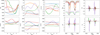 |
Fig. 1 Examples of the Stokes profiles (first two columns) and the model atmospheres (last three columns) used for training SENTIS. The solid lines represent the original data, and the dashed lines represent the reconstructed lines using the VQ-VAE model. |
3 Autoregressive neural machine translation
We considered the inference of atmospheric parameters from the interpretation of the Stokes profiles as a machine-translation problem. Given a sequence S = {S1, S2,…, SN} of length N that represents the Stokes parameters (whether the concatenated four Stokes parameters or a specific tokenization of them), the purpose of the model was to provide a probability distribution p(θ|S) over a sequence θ of length M that represents the model atmosphere (whether the concatenated stratifications or a specific tokenization of them). Having access to the probability distribution produces a generative model that can be used to sample from the posterior distribution. It is customary to use autoregressive models to solve this problem. These models encode the full posterior distribution as a product of conditional distributions,
 (2)
(2)
This means that the model is trained to predict the next token in the sequence given all previous tokens and the information about the Stokes parameters. The translation is typically done using an encoder-decoder architecture. An encoder uses S as input and produces a latent representation that is assumed to encode all the relevant information needed for the translation. The decoder takes this latent representation and produces in an autoregressive way an estimation of p(θi|θ1,…, θi−1, S).
When the model θ is chosen to be the full depth stratification of the model atmosphere, that is, θ = {T, v, vmic, Bx, By, Bz}, where x = {x(log τ500,1),…, x(log τ500,M)} for all variables x, this creates a regression problem because the model θ is continuous. In this case, we need to pre-define a functional form for the probability distribution p(θi|θ1,…, θi−1, S), which is not known in advance. For this reason, we considered a different approach.
We used a tokenization of the model atmosphere and the Stokes parameters (although that of the Stokes parameters is not mandatory). This tokenization introduces two desirable side effects. First, it is a very efficient way of compressing the information of the model atmosphere (and Stokes parameters) using a finite set of features. The power of tokenization lies in the fact that this compression is learned, as described in Sect. 3.1, from the training data, and it allows us to represent the model atmosphere and the Stokes parameters as finite sequences of tokens extracted from a fixed and finite code book. The second side effect is that the tokenization allows us to transform the problem into a classification problem, so that we can use a categorical distribution for the conditional probabilities,
 (3)
(3)
where Cat(θi|θ1,…, θi−1, S) is the categorical distribution over the set of tokens that represents the model atmosphere. Treating the problem as a categorical or classification one allows us to easily define the full posterior distribution, and we thus obtained a properly defined generative model.
We note that the translation problem is completely symmetric, so that it is straightforward to also consider the inverse problem. In this case, we considered the Stokes parameters as the target sequence and the model atmosphere as the input sequence. We consider this option in Sect. 6, where we obtain a generative model that can be used to produce emulated synthetic Stokes profiles from a model atmosphere, equipped with an uncertainty estimate.
3.1 Tokenizers
The wavelength variation in the Stokes parameters contains redundant information and is strongly compressible (see, e.g., Asensio Ramos et al. 2007b). Dimensionality reduction techniques such as a principal component analysis (PCA) or autoen-coders can be used to compress the Stokes parameters into a smaller set of features (Rees et al. 2000; Socas-Navarro 2005a; Casini et al. 2005). The same idea applies to the model atmosphere, as demonstrated by the success of inversion codes such as SIR, which parameterize the model atmosphere with only a few nodes.
Since classical dimensionality reduction methods such as the PCA or autoencoders are not suitable for the autoregressive translation problem because they provide a continuous representation of the data, we drew upon VQ-VAE (van den Oord et al. 2017) to learn a tokenization of the Stokes parameters and the model atmosphere. VQ-VAEs are a type of variational autoen-coder (autoencoder with a prescribed prior on the latent space) that learns a discrete representation of the data by mapping the continuous latent space produced by the encoder to a finite set of discrete tokens from a learned code book (see Fig. 2). The encoder E maps the input data (every Stokes parameter and physical variable, properly normalized) to a latent representation (di) of reduced spatial size but increased dimensionality (D). Specifically, the encoder first applies a 1D CNN layer with a kernel of size 3 that projects the 1D vector into a space of dimension 64 for the model parameters and 256 for the Stokes parameters. We verified that using a lower value for the Stokes parameters did not produce sufficiently good reconstructions. A consecutive application of three blocks containing a 1D convolutional layer with a kernel of size 3, GELU activation function (Hendrycks & Gimpel 2016), another 1D convolutional layer with a kernel of size 3 and a max pooling operation, were applied to reduce the spatial size of the vectors. A final 1D convolutional layer with a kernel of size 1 projects the latent representation to the desired dimension D = 8. Since the Stokes parameters for the Fe I spectral region contains 112 wavelength points, we finally had vectors with a size of 112/23 = 14. Likewise, the Ca II spectral region contained 96 wavelength points, which were therefore reduced to vectors with a size of 96/23 = 12. The model parameters were defined at 80 optical depth points, so that the spatial dimension was 80/23 = 10. We point out that we did not carry out a systematic search for the optimal specific architectures of the encoder and decoder because we only wished to demonstrate the feasibility of the approach. An architecture based on transformer encoders might be able to deal with Stokes parameters and model parameters sampled at arbitrary wavelengths and optical depths, but this is left for future work.
The latent representation was then quantized to the nearest token in the code book 𝒞, which is a set of K = 256 discrete vectors (ei) of dimension D = 8. The quantization was made by computing the ℓ2 distance between the latent representation and all the tokens in the code book, and selecting the token with the smallest distance. This meant that every Stokes parameter was described by a sequence of 14 tokens for the Fe I doublet and 12 tokens for the Ca II line, as extracted from the code book. The same applies to the model parameters, which were described by a sequence of 10 tokens. These tokens play a role similar to the nodes used in inversion codes such as SIR. The advantage is that, once learned, the tokenization can produce stratifications with the whole range of complexity and variability present in the training set, without the need to prescribe the number of nodes for the model atmosphere. As a final step, the quantized representation was then passed to the decoder Ɗ, which was a mirror of the encoder, using a linear upsampling operation instead of max pooling to increase the spatial size of the vectors. The Stokes parameters and the model parameters were both normalized before they were encoded with the VQ-VAE with the following formula:
 (4)
(4)
The values of xmin and xmax for each parameter are listed in Table 2.
The VQ-VAE was trained to minimize the reconstruction error between the input data and the output of the decoder, measured with the mean squared error, while making efficient use of the discrete code book (for details, see van den Oord et al. 2017). Noise with a standard deviation of 10−3 in units of the continuum intensity was added to the Stokes profiles during training. No noise was added to the atmospheric models. The VQ-VAE was trained with a batch size of 256 using the Adam optimizer (Kingma & Ba 2015) with a learning rate of 3 × 10⁻⁴, which was reduced following a cosine annealing law until it reached 3 × 10⁻⁵ after 30 epochs. The VQ-VAE reproduced the Stokes parameters and the model parameters from the quantized representation very well, as shown in Fig. 1. The dashed curves in Fig. 1 show the reconstructions, which overlap the original curves almost perfectly.
We note that the tokens of the physical parameters obtained by VQ-VAE were ordered starting from the deepest layer in the solar atmosphere, that is, the first token corresponded to the quantities at log τ500 = 1.5. This was convenient for the autore-gressive translation model because the variability of the models in the deep layers is far weaker than in the upper layers.
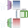 |
Fig. 2 VQ-VAE model we used for the tokenization. The encoder ℰ produces a latent representation of the Stokes parameters and the model stratifications, which is then passed through the decoder Ɗ after quantization with the aid of a learned code book. |
Normalization of the Stokes parameters and the model parameters before entering the VQ-VAE used for tokenization.
3.2 Transformer encoder-decoder
The transformer encoder-decoder architecture (Vaswani et al. 2017) is the backbone of the autoregressive translation model.
The encoder is a stack of four transformer encoder blocks, each of which contains a multihead self-attention layer and a feed-forward neural network. The self-attention layer allows the model to learn the relations between the tokens in the input sequence, while the feed-forward neural network applies a non-linear transformation to the output of the self-attention layer. We did not systematically search for the optimal hyperparameters of the transformer architecture either, but used eight heads in the self-attention layer, and the feed-forward neural network used a hidden layer with a size of 1024.
The input to the encoder is the concatenation of the token indices computed with the VQ-VAE for each one of the four Stokes parameters. The total sequence length was then 56 tokens for the Fe I spectral region and 48 when the Ca II spectral region was used alone. When more than one spectral region was used, we simply concatenated the token indices of the different spectral lines. In our case, the maximum sequence length was 104 when we considered the two spectral regions. Although the number of input tokens in our case was always fixed, we preferred to use specific tokens to indicate the start of sentence (SOS) and end of sentence (EOS), in anticipation of future work that will require the model to handle variable-length sequences for arbitrary combinations of different spectral lines at arbitrary wavelength samplings. The encoder then used an internal (learned) embedding representation with 256 + 2 vectors of dimension D = 256. The additional two vectors were associated with the SOS and EOS tokens.
We added the standard positional encoding (see, e.g., Vaswani et al. 2017) to the input sequence to provide the model with information about the order of the tokens in the sequence
 (5)
(5)
where j is the index in the sequence, and i indexes the dimension D. We discarded for the moment the use of any positional encoding extracted from the wavelength position, but we anticipate that it will be useful when lines observed with different instruments are used. Finally, the output of the encoder was a sequence of latent vectors zi of dimension D = 256 that represent the information extracted from the Stokes parameters that was used by the decoder to produce the model parameters.
The decoder was again a stack of four transformer decoder blocks, each of which contained a masked multihead self-attention layer, a multihead self-attention layer, and a feed-forward neural network. The masked self-attention layer allowed the model to learn the relations between the input tokens and the decoder, only attending to the tokens before the one under consideration, so that the proper conditional probability distribution of Eq. (3) was learned. The self-attention layer allowed the model to attend to the zi encoder latent vectors and learn how they affect the output sequence. The output of the decoder is a sequence of categorical probability distributions over the tokens ēi in the code book 𝒞 for the model stratifications. The decoder produced the output sequence in an autoregressive way and predicted the next token in the sequence based on the previous tokens and the latent vectors zi. In order to initiate the generation process, the decoder was called with a SOS token, and the output sequence was generated one token at a time until the EOS token was produced. Positional encoding was also added to the input sequence of the decoder.
The transformer encoder-decoder architecture is shown in Fig. 3. The transformer blocks were implemented using the nn.TransformerEncoderLayer and nn.TransformerDecoderLayer classes in PyTorch (Paszke et al. 2019). The transformer encoder-decoder was trained to minimize the cross-entropy loss between the output of the decoder and the target model parameters, which were also represented in the tokenized form. We used the Adam optimizer for the training, with a learning rate that was warmed-up from 3 × 10⁻⁷ to 3 × 10⁻⁴ in the first 50 epochs. It was then annealed using a cosine law until it reached 3 × 10⁻⁵ after 1000 epochs. We used a batch size of 512 and trained the model in mixed precision, using half-precision (fp16) and loss scaling, which took advantage of the increased speed and reduced memory impact in modern GPUs, such as the NVIDIA L40s and RTX4090 we used.
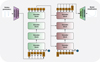 |
Fig. 3 Complete model, including the VQ-VAE encoder and decoder for tokenization and reconstruction, and the encoder-decoder architecture that translates the latent representations of the input and output spaces. The encoder and decoder blocks are both transformer layers. |
4 Validation
4.1 Inference of model stratifications
In order to determine the capabilities of the trained model, we used the test set of 6000 models and their corresponding Stokes profiles. Although extracted from the same distribution as the training set, they were never used during training. We explored two options to produce the output autoregressive sequence with the decoder. The first option was greedy decoding, in which the token with the highest probability is selected at each step. This produces a single deterministic output model. The second option was sampling, in which every token is sampled from the estimated categorical distribution at each step. Since this token was used as input to the decoder in the next step, the output is stochastic. When the decoder is called many times, it produces an ensemble of model stratifications that can be used to estimate the uncertainty in the solution.
Figures 4 and 5 show the results for the stratification of thermodynamical and magnetic quantities inferred from six profiles examples from the test set, respectively. In both figures, the upper three rows display the results when only the Fe I doublet at 630 nm is used, the middle three rows show the results when only the Ca II line at 8542 Å is used, and the last three rows show the results when both spectral regions are used. The blue curve is the original model stratification. The red curve is the result from the greedy decoding. The orange curves are 100 samples from the generative model. These models are represented with a low opacity, so that the zones with higher probability are more visible. The green curve is the median of the samples.
The results for the Fe I doublet show that the greedy solution and the median of the samples obtained from the distribution produce a good approximation to the original model in the line formation region for the doublet, which is located between log τ500 = 0 and log τ500 = −2.5 (see, e.g., Orozco Suárez et al. 2010; Borrero et al. 2014). The uncertainty on the solution is also much smaller in these regions than in the remaining atmosphere. The opposite occurs in the upper photosphere and chromosphere, where the uncertainties become larger because the Fe I doublet is barely sensitive to the specific physical conditions in these regions. The greedy and the median solution still often overlap with the original model in the upper regions of the atmosphere. This might simply be a consequence of the prior distribution inherent to the training data, which is based on the perturbation of semi-empirical models. These models already contain strong height correlations (e.g., the temperature increases in the chromosphere when the lower part of the atmosphere is similar to that of a quiet-Sun model). When the construction of the training data avoids using these semi-empirical models as a baseline, the resulting inferred models will surely be less informative in the upper layers of the atmosphere.
The results for the Ca II line at 8542 Å clearly demonstrate that the chromospheric line contains much more information about the physical conditions in the upper layers of the atmosphere, so that the inferred models are much more constrained in the chromosphere. We recall that the core of the Ca II line is sensitive to heights in the range between log τ500 ≈ −1.5 and log τ500 ≈ −4.0 (see, e.g., Quintero Noda et al. 2016). On the other hand, the uncertainties in the deeper layers of the atmosphere are larger than in the case of the Fe I doublet, which is a consequence of the fact that the Ca II line is very broad and the synthesized wavelength range does not reach continuum wavelengths. The inference in the two spectral regions clearly demonstrates that the microturbulent velocity is only poorly constrained. Microturbulent velocities are known to be quite degenerate with the temperature. Although the effect on the Stokes profiles is slightly different, it is hard to disentangle the two contributions with a few spectral lines. For this reason, it remains vaguely constrained. The magnetic field vector seems to be better constrained with the chromospheric line, however.
Although this is not surprising, it is worth noting that the generative model has learned to produce model atmospheres that are much more consistent with the original ones when the two spectral regions are used together. The inferred models look like a combination of the results obtained with the Fe I doublet and the Ca II line separately. The uncertainties are small in the deeper layers of the atmosphere because of the information that is provided by the Fe I doublet, while the chromospheric line provides a much better constraint in the upper layers of the atmosphere. The case of the temperature and LOS velocity stratifications is particularly interesting because some of the inferred models contain almost no uncertainty throughout the whole atmosphere (e.g., the first and last column). Other cases remain uncertain in the upper layers of the atmosphere (e.g., the fourth column).
4.2 Posterior check of synthetic Stokes profiles
Bypassing the whole nonlinear inversion of the radiative transfer equation has the undesired consequence of not explicitly forcing the Stokes profiles to be fit during the process. This is in contrast to what happens with classical iterative inversion methods (see, e.g., Asensio Ramos & Díaz Baso 2019). This verification needs to be done a posteriori by synthesizing the Stokes profiles from the inferred model and comparing them with the original Stokes profiles. If no good fitting is obtained, there is currently no way to improve the ML solution, but the solution provided by the ML method might be as a first guess for a classical inversion code (Gafeira et al. 2021). Other options can be based, for instance, on test-time computing (making the output of the ML model self-correct by using the Stokes profiles as input). Although they are very interesting and need to be explored in the future, they are beyond the scope of this work.
Figure 6 shows the results of the synthesis of the Fe I doublet on the inferred models using the Fe I observations in the test set shown in Figs. 4 and 5. The blue curves are the original Stokes profiles, the green and red curves are obtained in the median and greedy-decoded models, while the orange curves represent synthesis in the samples from the generative model. The synthesis is done using Hazel2 under the assumption of LTE, in the same conditions of the generation of the training set. The similarity between the original and the synthesized Stokes profiles is very good, which shows again that the relevant part of the inferred models is well constrained by the model.
5 Inversion of Hinode SOT/SP observations
The results of the validation are promising. We therefore applied the trained model to the inversion of Hinode SOT/SP observations. We inverted the observations of AR10953, which were obtained on May 1, 2007 almost at disk center. We used the scan that started at 16:30. The observations were obtained in fast-scanning mode, in which the pixel size is 0.32 arcsec. The level-1 data were used without any modification, but we normalized them by the intensity of the surrounding quiet Sun. After the Stokes profiles were properly normalized, they were tokenized using the pre-trained VQ-VAE, passed to the encoder, and then decoded by the decoder. The output sequence was then decoded using the VQ-VAE decoder to produce the model parameters.
We applied SENTIS to the whole field of view (FoV), which contains 512×512 pixels. Figure 7 shows the most interesting subfield of the whole FoV. We display the inferred physical quantities at two heights in the atmosphere, log τ500 = 0, which is very close to the formation height of the continuum (first four rows), and log τ500 = −1.5, which is closer to the formation height of the core of the lines (last four rows). The information obtained by our model at each optical depth surface was summarized with the median (MED) of the samples, together with the median absolute deviation (MAD) of the samples, which is an estimator of the standard deviation that is robust to outliers. We used robust estimates because we verified that some of the stratifications produced by the model can be considered outliers. This is the equivalent of the so-called hallucinations that are often found in generative models, which might eventually be reduced by using increasingly larger training sets. We compare the results of the new inversion code with those obtained using the classical SIR inversion code (in our case, via the Hazel2 inversion code), displayed in the third and seventh rows, and those obtained with the SICON inversion code (Asensio Ramos & Diaz Baso 2019), in the fourth and eighth rows. The results of SICON are crisper because the code automatically applies a deconvolution to the Stokes profiles, which is not the case of SIR or the new inversion code. For spatially deconvolved data, it is straightforward to use the approach of Ruiz Cobo & Asensio Ramos (2013) (see also Quintero Noda et al. 2015) by first applying a regularized deconvolution to the Stokes profiles and then inverting them.
The resemblance between the inferred models and the SIR models is very good, as shown by the Pearson correlation coefficients displayed in the panels that use SIR as the ground truth. The contrast of the plage that surrounds the sunspot is slightly lower for the temperature in our inversion than in the SIR inversion when observed at log τ500 = −1.5. The uncertainty is also larger in these zones, however. Conversely, the temperature estimate close at log τ500 = 0 is very certain. Likewise, the LOS velocity maps also correlate very well. In order to remove potential differences in the zeropoint of the LOS velocity, we subtracted the mean value of the LOS velocity in the FoV. Strong redshifts are found in the limb-side penumbra (located on the left side of the images) in both inversions. Larger uncertainties are correlated with the strong redshifts. SIR also recovers redshifts in the center-side penumbra (located on the right side of the images), however, which are not present in our inversion, even when the uncertainties are taken into account. The strong redshift of the most notable light bridge is common in the two inversions.
Strong similarities are found for all Cartesian components of the magnetic field. One obvious advantage of SENTIS is that artifacts visible in the SIR inversion in the Bx and By components are removed. They are strongly correlated with the location of the plage. This is a consequence of the well-known bias in the estimation of the transverse magnetic field from noisy Stokes Q and U profiles (Martínez González et al. 2012), which is proportional to the broadening of the spectral line. This bias is also absent from the SICON inversion, in this case because we exploited the spatial correlation of the magnetic field vector. The inferred Bx and By components are similar for the three codes. The results for the longitudinal component of the magnetic field are also very similar. The only difference is that the inferred Bz component in SIR is slightly larger in the plage regions. Finally, because the observation is of good quality and the Stokes parameters have a good signal-to-noise ratio, the results show good spatial coherence even though the inversions were carried out pixel by pixel.
In order to further validate the results, we selected three pixels in the FoV that are marked with blue, green and purple symbols in Fig. 7 and show their results in detail. The observed Stokes profiles in these pixels are shown with dots in the left-most four panels of Fig. 8. The semi-transparent curves show the Stokes profiles synthesized in the models inferred with SENTIS, while the median of the synthetic Stokes profiles is shown in solid color. The results display a very good agreement between the observed and the synthesized Stokes profiles, even though this is a fully a posteriori check. The inferred models (with 10 runs of the decoder) are shown in the rightmost panels of Fig. 8. Again, the distributions have a lower uncertainty in the line formation region, while the uncertainty increases toward the upper layers of the atmosphere.
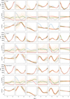 |
Fig. 4 Samples from the generative model (orange curves) for the inversion of six Stokes profiles extracted from the test set. The blue curve shows the original model, the green curve shows the median model, and the red curve shows the greedy decoded model. The upper three rows show the results when the Fe I spectral region was used, the middle three rows show the results when the Ca II spectral region was used, and the last three rows show the results when both spectral regions were used. |
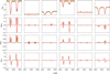 |
Fig. 6 Synthesis of the Stokes profiles (orange curves) emerging from the models shown in Figs. 4 and 5. The blue curves show the original Stokes profiles, and the green and red curves show the median Stokes profiles and the greedy decoded Stokes profiles, respectively. |
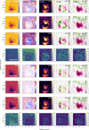 |
Fig. 7 Inversion results for the AR10953 at two different optical depths for SIR, SICON, and SENTIS. Given the probabilistic nature of SENTIS, we show the MED and MAD of the samples. The Pearson correlation coefficients between SIR and SENTIS and SICON are shown in the upper right corner of each panel. |
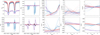 |
Fig. 8 Synthesis of the Stokes profiles in the models inferred by SENTIS in the three pixels marked in Fig. 7. The dots indicate the observed Stokes profiles, the semitransparent curves show the samples from the generative model, and the solid curves show the median of the samples. The colors correspond to the symbols in Fig. 7. |
6 Fast synthesis
Because the encoder-decoder architecture of Fig. 3 is a sequence-to-sequence model, it can also be used in reverse, as we described above. In other words, the tokenized model stratifications can be used as input, while the output of the model are the tokenized Stokes parameters. After passing through the VQ-VAE decoder, they were transformed into Stokes parameters for the spectral region of interest. This is, in summary, a generative model for the Stokes parameters, a stochastic synthesizer. This model can then be used for different purposes: For a fast synthesis of Stokes profiles for a large number of models, MCMC sampling of the posterior distribution for Bayesian inference, and so on. A summary of the results is displayed in Fig. 9. The blue curves are the original Stokes profiles in the model stratification of six models from the test set, the orange curves are the samples from the generative model, while the green curves represents the median of the samples. The green and blue curve overlap almost perfectly. Some large uncertainties remain, however (e.g., the circular polarization profile of the last column). Our hypothesis is that these artifacts can be reduced by using a larger training set and/or using a larger encoder-decoder model (e.g., more transformer blocks or larger dimension of the latent vectors).
7 Conclusions
We have explored the use of autoregressive neural machine translation models to accelerate the inversion of Stokes profiles. The model is based on the use of a vector-quantized variational autoencoder for tokenization of the Stokes parameters and the model stratifications. Stokes profiles and model stratifications are then represented as sequences of tokens, like sentences in a natural language. The translation is performed using a transformer encoder-decoder architecture under an autoregressive approach, which becomes a generative model given the stochastic nature of the decoder.
We demonstrated that the trained model can be used to reliably infer the stratification of the physical conditions in the solar atmosphere. The results are compatible with those obtained with classical inversion codes, but the inference is much faster. The model run time is independent of the complexity of the line formation process, and its ideal target application therefore is to quickly infer the thermodynamical and magnetic stratification from lines whose formation is dominated by non-LTE or partial frequency redistribution effects. Additionally, given the generative character of the model, it provides a way of sampling from the probability distribution of the model stratification, which allows us to estimate the uncertainty in the solution. As a guidance for the speed of the model, we reached a rate of ~ 125 inversions per second in a single NVIDIA 4090 GPU and generated ten samples per inversion. This is currently well beyond the reach for classical inversion codes, which typically take several seconds (e.g., SIR) or several minutes (e.g., Nicole or STiC) to invert a single Stokes profile.
We also demonstrated that the model can be used to carry out multiline inversions by simply concatenating the tokenized Stokes parameters of the different spectral lines. The model produces much better constrained models when more spectral lines are added. This reveals that the model has learned to exploit the information provided by the different spectral lines in a complementary way. Finally, when the encoder-decoder model is used in reverse, it can also be trained for the fast synthesis of Stokes profiles.
Even though the model is fast, transformer-based architectures are still computationally expensive because the self-attention mechanism scales quadratically with the number of tokens in the sequence. Because current advanced natural language models are based on exactly the same architecture, many techniques have been developed to reduce the computational cost of the model. For example, KV caching can be used (Pope et al. 2023), which allows the model to reuse the calculations performed for the attention when generating the next token, or linear attention mechanisms (e.g., Shen et al. 2018), which reduce the computational cost of the attention mechanisms.
The model we presented is of the encoder-decoder type, as usual in neural machine translation. Recent studies have shown, however, that decoder-only architectures can also be used for autoregressive translation (e.g., Gao et al. 2022; Fu et al. 2023).
Using a decoder alone might reduce the computational cost of the model because no encoder is needed. The decoder-only architecture can be trained by concatenating the tokenized Stokes parameters and the model stratifications, and then predicting the next token in the sequence given the previous tokens. The model can then be used to produce the model stratifications when the Stokes parameters are provided as context. We will explore this architecture in future works.
Sequence-to-sequence models represent a very powerful tool for the inversion of Stokes profiles because the sequence is arbitrary. These models can seamlessly deal with the concatenation of the tokenization of Stokes parameters of several spectral lines at arbitrary wavelength samplings when the relevant information is passed to the encoder. The main obstacle is the development of a dictionary of tokens that can deal with arbitrary spectral lines at arbitrary wavelength samplings for arbitrary instruments. A single VQ-VAE tokenization for all spectral lines might be envisioned, modifying the encoder and decoder to deal with the arbitrary wavelength sampling. Either 1D convolutional layers with appended wavelength information or transformer encoder and decoders might be used for this purpose. Another option is to use a different VQ-VAE tokenization for each spectral line, which would allow the model to learn the relevant information for each spectral line independently, at the expense of increasing the code book size. We anticipate that tokenization coupled with generative models (either autoregressive or based on other ideas, e.g., diffusion models) will produce significant advances in the inversion of Stokes profiles in the near future for single-pixel inversions and for the inversion of large data cubes.
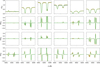 |
Fig. 9 Samples from the generative model of the synthesis neural translation model. |
Acknowledgements
AAR acknowledges funding from the Agencia Estatal de Investigación del Ministerio de Ciencia, Innovación y Universidades (MCIU/AEI) under grant “Polarimetric Inference of Magnetic Fields” and the European Regional Development Fund (ERDF) with reference PID2022-136563NB-I00/10.13039/501100011033. The Institute for Solar Physics is supported by a grant for research infrastructures of national importance from the Swedish Research Council (registration number 2021-00169). JdlCR gratefully acknowledges funding by the European Union through the European Research Council (ERC) under the Horizon Europe program (MAGHEAT, grant agreement 101088184). We also acknowledge the contribution of the IAC High-Performance Computing support team and hardware facilities to the results of this research. Part of the computations were enabled by resources provided by the National Academic Infrastructure for Supercomputing in Sweden (NAISS), partially funded by the Swedish Research Council through grant agreement no. 2022-06725, at the PDC Center for High Performance Computing, KTH Royal Institute of Technology (project numbers NAISS 2024/1-14 and 2025/1-9) This research has made use of NASA’s Astrophysics Data System Bibliographic Services. We acknowledge the community effort devoted to the development of the following open-source packages that were used in this work: numpy (numpy.org, Harris et al. 2020), matplotlib (matplotlib.org, Hunter 2007), PyTorch (pytorch.org, Paszke et al. 2019), scipy (scipy.org, Virtanen et al. 2020) and scikit-learn (scikit-learn.org, Pedregosa et al. 2011).
References
- Ardizzone, L., Kruse, J., Wirkert, S., et al. 2018, arXiv e-prints [arXiv:1808.04730] [Google Scholar]
- Asensio Ramos, A., & Díaz Baso, C. J. 2019, A&A, 626, A102 [NASA ADS] [CrossRef] [EDP Sciences] [Google Scholar]
- Asensio Ramos, A., Martinez Gonzalez, M. J., & Rubiño-Martín, J. A. 2007a, A&A, 476, 959 [NASA ADS] [CrossRef] [EDP Sciences] [Google Scholar]
- Asensio Ramos, A., Socas-Navarro, H., López Ariste, A., & Martínez González, M. J. 2007b, ApJ, 660, 1690 [NASA ADS] [CrossRef] [Google Scholar]
- Asensio Ramos, A., Trujillo Bueno, J., & Landi Degl’Innocenti, E. 2008, ApJ, 683, 542 [Google Scholar]
- Asensio Ramos, A., Cheung, M. C. M., Chifu, I., & Gafeira, R. 2023, Living Rev. Sol. Phys., 20, 4 [Google Scholar]
- Auer, L. H., Heasley, J. N., & House, L. L. 1977, Sol. Phys., 55, 47 [Google Scholar]
- Borrero, J. M., Tomczyk, S., Kubo, M., et al. 2011, Sol. Phys., 273, 267 [Google Scholar]
- Borrero, J. M., Lites, B. W., Lagg, A., Rezaei, R., & Rempel, M. 2014, A&A, 572, A54 [NASA ADS] [CrossRef] [EDP Sciences] [Google Scholar]
- Campbell, R. J., Mathioudakis, M., & Noda, C. Q. 2025, arXiv e-prints [arXiv:2506.16810] [Google Scholar]
- Carroll, T. A., & Kopf, M. 2008, A&A, 481, L37 [NASA ADS] [CrossRef] [EDP Sciences] [Google Scholar]
- Carroll, T. A., & Staude, J. 2001, A&A, 378, 316 [NASA ADS] [CrossRef] [EDP Sciences] [Google Scholar]
- Casini, R., Bevilacqua, R., & López Ariste, A. 2005, ApJ, 622, 1265 [Google Scholar]
- Centeno, R., Flyer, N., Mukherjee, L., et al. 2022, ApJ, 925, 176 [NASA ADS] [CrossRef] [Google Scholar]
- Collados, M., Martinez Pillet, V., Ruiz Cobo, B., del Toro Iniesta, J. C., & Vazquez, M. 1994, A&A, 291, 622 [Google Scholar]
- de la Cruz Rodríguez, J. 2019, A&A, 631, A153 [NASA ADS] [CrossRef] [EDP Sciences] [Google Scholar]
- de la Cruz Rodríguez, J., & van Noort, M. 2017, Space Sci. Rev., 210, 109 [Google Scholar]
- de la Cruz Rodríguez, J., Leenaarts, J., Danilovic, S., & Uitenbroek, H. 2019, A&A, 623, A74 [Google Scholar]
- del Toro Iniesta, J. C., & Ruiz Cobo, B. 2016, Living Rev. Sol. Phys., 13, 4 [Google Scholar]
- del Toro Iniesta, J. C., Tarbell, T. D., & Ruiz Cobo, B. 1994, ApJ, 436, 400 [CrossRef] [Google Scholar]
- Díaz Baso, C. J., Asensio Ramos, A., & de la Cruz Rodríguez, J. 2022, A&A, 659, A165 [NASA ADS] [CrossRef] [EDP Sciences] [Google Scholar]
- Díaz Baso, C. J., Asensio Ramos, A., de la Cruz Rodríguez, J., da Silva Santos, J. M., & Rouppe van der Voort, L. 2025, A&A, 693, A170 [NASA ADS] [CrossRef] [EDP Sciences] [Google Scholar]
- Fontenla, J. M., Avrett, E., Thuillier, G., & Harder, J. 2006, ApJ, 639, 441 [Google Scholar]
- Fontenla, J. M., Curdt, W., Haberreiter, M., Harder, J., & Tian, H. 2009, ApJ, 707, 482 [Google Scholar]
- Frutiger, C., Solanki, S. K., Fligge, M., & Bruls, J. H. M. J. 2000, A&A, 358, 1109 [NASA ADS] [Google Scholar]
- Fu, Z., Lam, W., Yu, Q., et al. 2023, arXiv e-prints [arXiv:2304.04052] [Google Scholar]
- Gafeira, R., Orozco Suárez, D., Milic, I., et al. 2021, A&A, 651, A31 [NASA ADS] [CrossRef] [EDP Sciences] [Google Scholar]
- Gao, Y., Herold, C., Yang, Z., & Ney, H. 2022, in Proceedings of the 2nd Conference of the Asia-Pacific Chapter of the Association for Computational Linguistics and the 12th International Joint Conference on Natural Language Processing (Volume 1: Long Papers), eds. Y. He, H. Ji, S. Li, Y. Liu, & C.-H. Chang (Online only: Association for Computational Linguistics), 562 [Google Scholar]
- Gingerich, O., Noyes, R. W., Kalkofen, W., & Cuny, Y. 1971, Sol. Phys., 18, 347 [Google Scholar]
- Grevesse, N., & Sauval, A. J. 1999, A&A, 347, 348 [NASA ADS] [Google Scholar]
- Harris, C. R., Millman, K. J., van der Walt, S. J., et al. 2020, Nature, 585, 357 [NASA ADS] [CrossRef] [Google Scholar]
- Hendrycks, D., & Gimpel, K. 2016, arXiv e-prints [arXiv: 1606.08415] [Google Scholar]
- Henighan, T., Kaplan, J., Katz, M., et al. 2020, arXiv e-prints [arXiv:2010.14701] [Google Scholar]
- Holweger, H., & Mueller, E. A. 1974, Sol. Phys., 39, 19 [NASA ADS] [CrossRef] [Google Scholar]
- Hunter, J. D. 2007, Comput. Sci. Eng., 9, 90 [NASA ADS] [CrossRef] [Google Scholar]
- Jarolim, R., Molnar, M. E., Tremblay, B., Centeno, R., & Rempel, M. 2025, ApJ, 985, L7 [Google Scholar]
- Kaplan, J., McCandlish, S., Henighan, T., et al. 2020, arXiv e-prints [arXiv:2001.08361] [Google Scholar]
- Kingma, D. P., & Ba, J. 2015, in ICLR (Poster), eds. Y. Bengio, & Y. LeCun [Google Scholar]
- Kleint, L., Berkefeld, T., Esteves, M., et al. 2020, A&A, 641, A27 [EDP Sciences] [Google Scholar]
- Kosugi, T., Matsuzaki, K., Sakao, T., et al. 2007, Sol. Phys., 243, 3 [Google Scholar]
- Landi Degl’Innocenti, E., & Landolfi, M., eds. 2004, Astrophysics and Space Science Library, 307, Polarization in Spectral Lines [Google Scholar]
- Lee, K.-S., Chae, J., Park, E., et al. 2022, ApJ, 940, 147 [Google Scholar]
- Lites, B. W., Elmore, D. F., Streander, K. V., et al. 2001, in Presented at the Society of Photo-Optical Instrumentation Engineers (SPIE) Conference, 4498, Proc. SPIE, UV/EUV and Visible Space Instrumentation for Astronomy and Solar Physics, eds. O. H. Siegmund, S. Fineschi, & M. A. Gummin, 73 [Google Scholar]
- Lites, B., Casini, R., Garcia, J., & Socas-Navarro, H. 2007, Mem. Soc. Astron. Italiana, 78, 148 [Google Scholar]
- Maltby, P., Avrett, E. H., Carlsson, M., et al. 1986, ApJ, 306, 284 [Google Scholar]
- Martínez González, M. J., Manso Sainz, R., Asensio Ramos, A., & Belluzzi, L. 2012, MNRAS, 419, 153 [CrossRef] [Google Scholar]
- Milic, I., & Gafeira, R. 2020, A&A, 644, A129 [NASA ADS] [CrossRef] [EDP Sciences] [Google Scholar]
- Milic, I., & van Noort, M. 2018, A&A, 617, A24 [Google Scholar]
- Mistryukova, L., Plotnikov, A., Khizhik, A., et al. 2023, Sol. Phys., 298, 98 [Google Scholar]
- Orozco Suárez, D., & Del Toro Iniesta, J. C. 2007, A&A, 462, 1137 [NASA ADS] [CrossRef] [EDP Sciences] [Google Scholar]
- Orozco Suárez, D., Bellot Rubio, L. R., & Del Toro Iniesta, J. C. 2010, A&A, 518, A3 [Google Scholar]
- Osborne, C. M. J., Armstrong, J. A., & Fletcher, L. 2019, ApJ, 873, 128 [NASA ADS] [CrossRef] [Google Scholar]
- Pastor Yabar, A., Borrero, J. M., & Ruiz Cobo, B. 2019, A&A, 629, A24 [NASA ADS] [CrossRef] [EDP Sciences] [Google Scholar]
- Paszke, A., Gross, S., Massa, F., et al. 2019, in Advances in Neural Information Processing Systems, 32, eds. H. Wallach, H. Larochelle, A. Beygelzimer, F. d’é Buc, E. Fox, & R. Garnett (Curran Associates, Inc.), 8024 [Google Scholar]
- Pedregosa, F., Varoquaux, G., Gramfort, A., et al. 2011, J. Mach. Learn. Res., 12, 2825 [Google Scholar]
- Pope, R., Douglas, S., Chowdhery, A., et al. 2023, in Proceedings of the Sixth Conference on Machine Learning and Systems, MLSys 2023, Miami, FL, USA, June 4-8, 2023, eds. D. Song, M. Carbin, & T. Chen (mlsys.org) [Google Scholar]
- Quintero Noda, C., Asensio Ramos, A., Orozco Suárez, D., & Ruiz Cobo, B. 2015, A&A, 579, A3 [NASA ADS] [CrossRef] [EDP Sciences] [Google Scholar]
- Quintero Noda, C., Shimizu, T., de la Cruz Rodríguez, J., et al. 2016, MNRAS, 459, 3363 [Google Scholar]
- Rasmussen, C. E., & Williams, C. K. I. 2006, Gaussian Processes for Machine Learning (The MIT Press) [Google Scholar]
- Rees, D. E., López Ariste, A., Thatcher, J., & Semel, M. 2000, A&A, 355, 759 [NASA ADS] [Google Scholar]
- Rimmele, T. R., Warner, M., Keil, S. L., et al. 2020, Sol. Phys., 295, 172 [Google Scholar]
- Ruiz Cobo, B., & Asensio Ramos, A. 2013, A&A, 549, L4 [NASA ADS] [CrossRef] [EDP Sciences] [Google Scholar]
- Ruiz Cobo, B., & del Toro Iniesta, J. C. 1992, ApJ, 398, 375 [Google Scholar]
- Ruiz Cobo, B., Quintero Noda, C., Gafeira, R., et al. 2022, A&A, 660, A37 [NASA ADS] [CrossRef] [EDP Sciences] [Google Scholar]
- Scharmer, G. B., Bjelksjö, K., Korhonen, T. K., Lindberg, B., & Petterson, B. 2003, in Proc. SPIE, 4853, Innovative Telescopes and Instrumentation for Solar Astrophysics, eds. S. L. Keil, & S. V. Avakyan, 341 [NASA ADS] [CrossRef] [Google Scholar]
- Scharmer, G. B., Sliepen, G., Sinquin, J.-C., et al. 2024, A&A, 685, A32 [NASA ADS] [CrossRef] [EDP Sciences] [Google Scholar]
- Scherrer, P. H., Schou, J., Bush, R. I., et al. 2012, Sol. Phys., 275, 207 [Google Scholar]
- Schmidt, W., von der Lühe, O., Volkmer, R., et al. 2012, Astron. Nachr., 333, 796 [Google Scholar]
- Shen, Z., Zhang, M., Zhao, H., Yi, S., & Li, H. 2018, arXiv e-prints [arXiv:1812.01243] [Google Scholar]
- Socas-Navarro, H. 2003, Neural Networks, 16, 355 [Google Scholar]
- Socas-Navarro, H. 2005a, ApJ, 620, 517 [Google Scholar]
- Socas-Navarro, H. 2005b, ApJ, 621, 545 [Google Scholar]
- Socas-Navarro, H., & Asensio Ramos, A. 2021, A&A, 652, A78 [NASA ADS] [CrossRef] [EDP Sciences] [Google Scholar]
- Socas-Navarro, H., Trujillo Bueno, J., & Ruiz Cobo, B. 2000, ApJ, 530, 977 [NASA ADS] [CrossRef] [Google Scholar]
- Socas-Navarro, H., de la Cruz Rodríguez, J., Asensio Ramos, A., Trujillo Bueno, J., & Ruiz Cobo, B. 2015, A&A, 577, A7 [NASA ADS] [CrossRef] [EDP Sciences] [Google Scholar]
- Solanki, S. K. 1986, A&A, 168, 311 [NASA ADS] [Google Scholar]
- Solanki, S. K., Rueedi, I. K., & Livingston, W. 1992, A&A, 263, 312 [Google Scholar]
- Uitenbroek, H. 2001, ApJ, 557, 389 [Google Scholar]
- van den Oord, A., Vinyals, O., & Kavukcuoglu, K. 2017, in Proceedings of the 31st International Conference on Neural Information Processing Systems, NIPS’17 (Red Hook, NY, USA: Curran Associates Inc.), 6309 [Google Scholar]
- van Noort, M. 2012, A&A, 548, A5 [NASA ADS] [CrossRef] [EDP Sciences] [Google Scholar]
- Vaswani, A., Shazeer, N., Parmar, N., et al. 2017, in Advances in Neural Information Processing Systems, 30, eds. I. Guyon, U. V. Luxburg, S. Bengio, et al. (Curran Associates, Inc.) [Google Scholar]
- Vernazza, J. E., Avrett, E. H., & Loeser, R. 1981, ApJS, 45, 635 [Google Scholar]
- Virtanen, P., Gommers, R., Oliphant, T. E., et al. 2020, Nat. Methods, 17, 261 [Google Scholar]
- Wang, R., Fouhey, D. F., Higgins, R. E. L., et al. 2024, ApJ, 970, 168 [Google Scholar]
- Xu, C., Wang, J., Li, H., et al. 2024, ApJ, 977, 101 [Google Scholar]
- Yang, K. E., Tarr, L. A., Rempel, M., et al. 2024, ApJ, 976, 204 [Google Scholar]
The diagonal term is used to stabilize the inversion of the covariance matrix, which is otherwise ill conditioned.
All Tables
Normalization of the Stokes parameters and the model parameters before entering the VQ-VAE used for tokenization.
All Figures
|
Fig. 1 Examples of the Stokes profiles (first two columns) and the model atmospheres (last three columns) used for training SENTIS. The solid lines represent the original data, and the dashed lines represent the reconstructed lines using the VQ-VAE model. |
| In the text | |
|
Fig. 2 VQ-VAE model we used for the tokenization. The encoder ℰ produces a latent representation of the Stokes parameters and the model stratifications, which is then passed through the decoder Ɗ after quantization with the aid of a learned code book. |
| In the text | |
|
Fig. 3 Complete model, including the VQ-VAE encoder and decoder for tokenization and reconstruction, and the encoder-decoder architecture that translates the latent representations of the input and output spaces. The encoder and decoder blocks are both transformer layers. |
| In the text | |
|
Fig. 4 Samples from the generative model (orange curves) for the inversion of six Stokes profiles extracted from the test set. The blue curve shows the original model, the green curve shows the median model, and the red curve shows the greedy decoded model. The upper three rows show the results when the Fe I spectral region was used, the middle three rows show the results when the Ca II spectral region was used, and the last three rows show the results when both spectral regions were used. |
| In the text | |
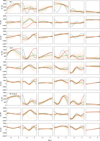 |
Fig. 5 Same as Fig. 4, but for the magnetic field components. |
| In the text | |
|
Fig. 6 Synthesis of the Stokes profiles (orange curves) emerging from the models shown in Figs. 4 and 5. The blue curves show the original Stokes profiles, and the green and red curves show the median Stokes profiles and the greedy decoded Stokes profiles, respectively. |
| In the text | |
|
Fig. 7 Inversion results for the AR10953 at two different optical depths for SIR, SICON, and SENTIS. Given the probabilistic nature of SENTIS, we show the MED and MAD of the samples. The Pearson correlation coefficients between SIR and SENTIS and SICON are shown in the upper right corner of each panel. |
| In the text | |
|
Fig. 8 Synthesis of the Stokes profiles in the models inferred by SENTIS in the three pixels marked in Fig. 7. The dots indicate the observed Stokes profiles, the semitransparent curves show the samples from the generative model, and the solid curves show the median of the samples. The colors correspond to the symbols in Fig. 7. |
| In the text | |
|
Fig. 9 Samples from the generative model of the synthesis neural translation model. |
| In the text | |
Current usage metrics show cumulative count of Article Views (full-text article views including HTML views, PDF and ePub downloads, according to the available data) and Abstracts Views on Vision4Press platform.
Data correspond to usage on the plateform after 2015. The current usage metrics is available 48-96 hours after online publication and is updated daily on week days.
Initial download of the metrics may take a while.