| Issue |
A&A
Volume 703, November 2025
|
|
|---|---|---|
| Article Number | A22 | |
| Number of page(s) | 14 | |
| Section | Stellar atmospheres | |
| DOI | https://doi.org/10.1051/0004-6361/202556223 | |
| Published online | 31 October 2025 | |
HE2159-0551: A very metal-poor peculiar low-Ba giant – a candidate from the LMS-1/Wukong
Goethe-Universität, Institute for Applied Physics,
Max-von-Laue-Straße 1,
60438
Frankfurt am Main,
Germany
★ Corresponding author: This email address is being protected from spambots. You need JavaScript enabled to view it.
Received:
2
July
2025
Accepted:
28
August
2025
Abstract
Aims. We present a comprehensive spectroscopic and kinematic analysis of the very metal-poor ([Fe/H] = −2.60 ± 0.20 dex) giant star HE2159-0551. By investigating the star’s chemodynamic characteristics, we seek to address its formation, evolution, and role in the chemical enrichment of the early cosmos and the possible connection to known merger events.
Methods. From high-resolution data, we performed a 1D, local thermodynamic equilibrium analysis using PyMoogi. We conducted a detailed abundance analysis of 23 elements (C, N, O, Na, Mg, Al, Si, K, Ca, Sc, Ti, V, Cr, Mn, Fe, Co, Ni, Zn, Sr, Y, Zr, Ba, and Eu) to derive abundances or place limits. Finally, we computed orbital parameters to investigate the kinematics and, thus, the nucleosynthetic origin of HE2159-0551.
Results. The analysis yields significant insights into the chemical composition of HE2159-0551, highlighting its peculiarities among very metal-poor stars. The star shows signs of internal mixing and a peculiar abundance pattern, particularly regarding the heavy elements. We find a low Ba abundance (s-process element) and a suppressed contamination of r-process elements, even though r-process enrichment may be expected in very metal-poor stars. The orbital parameters and kinematic properties indicate that HE2159-0551 is a thick disk star, connected to the old and metal-poor LMS-1/Wukong progenitor resulting from an early merger.
Conclusions. Our kinematic analysis suggests a potential connection of HE2159-0551 to the merger LMS-1/Wukong. We conclude that the nucleosynthesis processes responsible for the star’s enrichment in heavy elements are different from those observed in many other metal-poor stars, as neither the main r- nor s-process can explain the derived abundance pattern. A possible weak-r or vp-process forming Sr-Zr but not Ba might have mixed into a low level of underlying r-process material in the low-mass LMS-1/Wukong system.
Key words: nuclear reactions, nucleosynthesis, abundances / stars: abundances / stars: chemically peculiar / stars: kinematics and dynamics / stars: individual: HE2159-0551 / stars: Population II
© The Authors 2025
 Open Access article, published by EDP Sciences, under the terms of the Creative Commons Attribution License (https://creativecommons.org/licenses/by/4.0), which permits unrestricted use, distribution, and reproduction in any medium, provided the original work is properly cited.
This article is published in open access under the Subscribe to Open model. This email address is being protected from spambots. You need JavaScript enabled to view it. to support open access publication.
1 Introduction
Very metal-poor (VMP) stars, which exhibit a peculiar abundance pattern, are crucial for advancing our understanding of stellar and Galactic chemical evolution (GCE) and early nucleosynthesis. In particular, the rapid neutron-capture process (r-process) is responsible for producing half the heavy elements beyond iron early on. Its study is essential for unraveling the complexities of element formation in the cosmos (Burbidge et al. 1957; Christlieb et al. 2004; Arcones & Thielemann 2023). Stellar abundances of neutron-capture (n-capture) elements are particularly important for identifying the astrophysical sites of nucleosynthesis. The r-process forms Eu and is often linked to the explosive conditions of rare core-collapse (CC) supernovae (SNe) or neutron-star mergers (NSMs – or compact mergers) (e.g., Barklem et al. 2005; Winteler et al. 2012; Hansen et al. 2014, 2018b; Hotokezaka et al. 2018; Cowan et al. 2021). The detection of the r-process signature in the kilonova associated with the NSM event GW1708178 provides compelling evidence for an NSM to be a site of the r-process nucleosynthesis; based on one single event to date (e.g., Abbott et al. 2017; Watson et al. 2019). The weak r-process is a crucial nucleosynthesis process that occurs in environments such as neutrino-driven winds from CC SNe. This process might be responsible for the formation of certain elements up to Z ~ 50 and plays a significant role in the chemical evolution (Montes et al. 2007; Hansen et al. 2012; Arcones & Bliss 2014). The νp-process occurs in the neutrino wind from a hot proto-neutron star following a supernova (SN) explosion, providing a crucial environment for the synthesis of elements beyond Fe (Fröhlich et al. 2006; Fröhlich & Rauscher 2012). As the proto-neutron star cools and emits neutrinos, these particles interact with the surrounding stellar matter, creating proton-rich conditions that facilitate nucleosynthesis typically producing elements around Fe and beyond up to Sr-Zr, possibly reaching Ru (Fröhlich et al. 2006). Understanding the weak r- and νp-process is essential for elucidating the origins of the elements we observe, and detailed abundance patterns in metal-poor (MP) stars help us separate and understand these processes in more detail.
Following the classification from Beers & Christlieb (2005), VMP stars are defined as having [Fe/H] < −2.00 dex. The abundance patterns of these stars can vary significantly (see, e.g., the r-poor and r-rich stars analyzed by Honda et al. (2006) and Sneden et al. (2003), respectively), offering valuable insights into the stars’ origin and evolutionary histories (François et al. 2007; Hansen et al. 2012). These variations in r-process elements challenge existing theories by illuminating the history of chemical enrichment and mixing processes throughout a star’s life cycle. As stars ascend the giant branch, they can experience significant internal mixing processes and nucleosynthesis, which can alter their surface compositions (e.g., Korn et al. 2006, 2008; Pedersen et al. 2021; de Melo et al. 2024). Despite the potential insights from studying these stars, our understanding of the specific evolutionary pathways leading to unusual abundance patterns remains limited. Stars with enhanced C, N, and Ba abundances (e.g., Hansen et al. 2016, 2019; Zhang et al. 2023), the latter typically formed by the slow neutron-capture process (s-process), often reflect the products and mass-transfer of asymptotic giant branch (AGB) stars. However, some VMP giants display peculiar abundance patterns that deviate from established trends, raising critical questions about the mechanisms behind these anomalies (e.g., Sneden et al. 2003; Honda et al. 2006).
Significant fractions of the Milky Way’s stellar halo are composed of stars that originated in low-mass companions, ranging from dwarf spheroidals and ultra-faint dwarf galaxies to bound systems such as globular clusters, and were later accreted through gravitational interactions and mergers (e.g., Koppelman et al. 2019a; Aguado et al. 2021; Matsuno et al. 2022a,b). These accretion events are key to unraveling our Galaxy’s early assembly history, since each merger leaves behind distinctive chemical and dynamical signatures in the halo’s stellar populations. Recent studies using Gaia data and large-scale spectroscopic surveys, for example, APOGEE (Blanton et al. 2017) or GALAH (Buder et al. 2024), have revealed numerous stellar substructures associated with distinct past accretion events (e.g., Helmi et al. 2018; Naidu et al. 2020; Yuan et al. 2020). Among these newly identified substructures, the low-mass-stream-1 (LMS-1), a possible low-mass extension of Wukong1, stands out as a particularly interesting component due to its exceptionally low metallicity and polar orbital configuration (Yuan et al. 2020; Naidu et al. 2020; Malhan et al. 2021).
In this paper, we focus on the analysis of the chemically peculiar, VMP giant star HE2159-0551, whose kinematic and chemical properties suggest a connection to the LMS-1/Wukong merger event. We find that it exhibits an abundance pattern that deviates from the expected heavy element (Z > 30) trends observed in similar stars. Through a detailed chemodynamical analysis, we explore its possible association with LMS-1/Wukong, thereby refining our understanding of the interplay between accretion processes, Galactic dynamical evolution, and early nucleosynthesis. Understanding the origin of abundance peculiarities is crucial for refining models of stellar evolution and chemical enrichment in the early galaxy.
In Sect. 2, we present a brief overview of the observational data. Section 3 details the radial velocity (RV) computations, followed by the stellar parameters in Sect. 4. Section 5 describes the star’s kinematics, while Sect. 6 focuses on the chemical abundances of 23 elements. Section 7 presents the results and concludes the study.
2 Observations
We used high-resolution spectra obtained with the Ultraviolet and Visual Echelle Spectrograph (UVES) at the Very Large Telescope (VLT), observed over five nonconsecutive nights. The S/N is approximately 200 around 6060 Å and 30 around 3440 Å; for details on the spectra see Table A.1 in the appendix. The spectra cover a wavelength range from approximately 3000 Å to ~9500 Å with some gaps due to different arms and dichroics. The central wavelengths are 346 nm and 390 nm for the blue arm, and 564 nm, 580 nm, and 760 nm for the red arm. The UVES spectra undergo automatic reduction using the UVES pipeline, which includes bias correction, flat-fielding, sky subtraction, order merging, wavelength calibration, and background subtraction (Dekker et al. 2000). The star has a mean G magnitude of 12.0582 ± 0.0002 (Gaia Collaboration 2023) and the coordinates (J2000) are right ascension (RA): 22 02 16.3602355800 and declination (Dec): −05 36 48.534816816.
RV literature values and the uncertainties based on Hansen et al. (2015, 2018b) and the Gaia Collaboration (2016, 2023) compared to this work (single-file analysis (shifting) and CC method).
3 Radial velocity
We employed the Image Reduction and Analysis Facility (IRAF)2 (Tody 1986, 1993; Fitzpatrick et al. 2024) to compute the RV by analyzing each individual spectrum before coadding. We identified the Balmer lines in IRAF (using rvidlines), compared the observed wavelengths to their rest frame wavelengths to determine the RV, and later corrected for the barycentric velocity. We shifted the files based on this value. Table A.1 presents the RV value for each individual file. We found a final RV value of −106.40 ± 1.20 km s−1 as an average for all spectra and compared this computation to another method by using a cross-correlation (CC) method against the spectrum from July 28, 2015 (see Table A.1). This results in a RV of −107.00 ± 4.00 km s−1, agreeing with the RV result of our initial analysis3. Table A.1 reveals small differences in the individual RV values, which may be attributed to a slight reduction discrepancy. Notably, the largest discrepancy in RVs is observed in one file observed on July 28, 2015. The cross-correlation method yields −117.36 km s−1, while the single-file analysis results in −104.84 km s−1 after applying the barycentric correction (BC). There are sufficient lines available for cross-correlation, and the influence of telluric lines on the results is expected to be minimal as the spectra undergo sky subtraction, see Sect. 2.
The Gaia Collaboration (2016, 2023) report an RV of −106.38 ± 0.80 km s−1, with the uncertainty calculated as the standard error of the mean. Hansen et al. (2018b) give a value of −106.65 ± 0.88 km s−1, while Hansen et al. (2015) provide an RV value of −131.30 ± 0.80 km s−1. This RV value is comparable to the values we computed prior to applying the barycentric correction of 25.21 km s−1, see Table A.1. This indicates that the RV in Hansen et al. (2015) is given without the barycentric correction. Overall, our computed RV aligns well with the literature; see Table 1. Based on the above, we exclude binarity.
Stellar parameters in this study compared to that from Hansen etal. (2015).
4 Stellar parameters
We determined the stellar parameters spectroscopically using 20 Fe I and 14 Fe II lines from a known line list across a broad wavelength range. We list the individual lines and references in Table 4. For blended lines, we employed the deblending function in IRAF, as neglecting this step can result in significantly inaccurate abundance measurements. We generated our atmospheric model by interpolating Kurucz ATLAS9 models (Kurucz 1970; Castelli & Kurucz 2003), which we then used as input for PyMoogi4. The results of the stellar parameters are presented in Table 2, alongside the literature data from Hansen et al. (2015). We determined the statistical uncertainty on the metallicity as the standard deviation stemming from the Fe I lines using the final adopted atmospheric model in PyMoogi. For the other stellar parameters (microturbulence, surface gravity, and temperature) we computed detailed uncertainties (see Appendix B).
Following the methods outlined by Mucciarelli et al. (2013) and Hansen (2011), we derived the effective temperature by using Fe I and Fe II lines. We aimed for a flat slope in the abundance measurements of the examined lines (for both neutral and ionized Fe lines), regardless of the excitation potential of the lines. We computed an effective temperature of 5000 ± 140 K.
We used the abundance of Fe I to determine the star’s metallicity, based on the equivalent widths (EWs). While metallicity can be assessed using Fe I lines alone, these lines are more susceptible to nonlocal thermodynamic equilibrium (NLTE) effects compared to Fe II lines (Bergemann et al. 2012). However, the number of detectable Fe II lines is limited, which is why the determination of the metallicity by Fe II lines alone could be statistically unreliable. We derived [Fe/H] = −2.60 ± 0.20 dex in 1D, local thermodynamic equilibrium. The uncertainty reflects the systematic uncertainty of the Fe abundance. We double-checked the metallicity by synthesizing the Fe lines listed in Table 4.
We required ionization equilibrium between the Fe I and Fe II lines to determine the surface gravity. However, the surface gravity estimate may be biased, as Fe I is a non-dominant species in cool giants and could be affected by NLTE conditions, potentially introducing systematic errors in these measurements (Hansen 2011; Bergemann et al. 2011). We compute a log g of 1.80 ± 0.40 dex.
We assume that Fe I lines provide consistent Fe abundance measurements regardless of their individual strengths, implying no dependency between line strength and Fe abundance (Hansen 2011; Mucciarelli et al. 2013). We compute a microtur-bulence of 2.40 ± 0.30 km s−1. Following the empirical formula given by Mashonkina et al. (2017), we derive a microturbulence of 1.95 km s−1. Mashonkina et al. (2017) conclude that the empirical formula should only be used for extremely and ultra MP stars, while HE2159-0551 is a VMP star. Therefore, we keep the 2.40 km s−1 as the microturbulence.
We include the literature values of the stellar parameters from Hansen et al. (2015) in Table 2, alongside the values we derived. These values fall within the combined uncertainties. Notable differences, particularly in the effective temperature, likely arise from the different methods employed to derive the stellar parameters. We utilized a spectroscopic approach, while Hansen et al. (2015) employed a fitting method that matches spectrophotometric observations with model atmospheres. Following Mucciarelli & Bonifacio (2020), the differences between the stellar parameters of giant stars derived from spectroscopy and photometry increase with decreasing metallicity. The spectroscopic temperature for a star with [Fe/H] = −2.60 dex could be lower by around 350 K (Mucciarelli & Bonifacio 2020). We determine a spectroscopic effective temperature that is 200 K higher than the photometric value reported by Hansen et al. (2015).
Automated tools like xiru5 (Alencastro Puls 2023), a Python wrapper for the MOOG code, or ATHOS6 (A Tool for Homogenizing Stellar parameters, Hanke et al. 2018) have the potential to enhance precision; however, these tools often have limitations when it comes to individual parameters. We employed xiru to derive the stellar parameters based on the EW measurements. This analysis yielded the following results: Teff = 4785.40 ± 204.80 K, log g = 0.72 ± 1.11 dex, [Fe/H] = −2.95 ± 0.17 dex, and vt = 3.02 ± 0.36 km s−1. Notably, all derived stellar parameters are within combined uncertainties when comparing to our results presented in Sect. 4, reinforcing the reliability of our measurements. ATHOS returns similar or lower values than xiru, still within combined uncertainties compared to our results.
5 Kinematics
5.1 Computing orbital parameters
To compute the orbital parameters of an object, such as actions and energies (J, E), we required complete 6D phase-space measurements of our object. For the 2D sky position (α,δ) and the 2D proper motion ( ) along with the associated uncertainties, we used the data for HE2159-0551 from the Gaia DR3 dataset (Gaia Collaboration 2016, 2023), while the parameters for the heliocentric distance (D⊙) are based on the Bailer-Jones et al. (2021) catalog. The computed value for the RV is discussed in Sect. 3. The used 6D phase-space values and their uncertainties are shown in Table C.1 in the appendix.
We adopted the Galactic potential of McMillan (2017) to compute the orbits and orbital parameters of HE2159-0551. This time-independent, static, and axisymmetric model of the Milky Way contains a bulge, disk components, and the NFW (Navarro-Frenk-White) halo. To set the McMillan (2017) potential and to integrate the orbits, we made use of the galpy7 module (Bovy 2015). For every calculated orbit in this paper, we used the same total integration time of 10 Gyr, with time steps of 1 Myr. For further details we refer to Plonka et al. (in prep.). We took solar and local standard of rest (LSR) data from Bennett & Bovy (2018) and Schönrich et al. (2010), respectively.
Starting from GALAHDR4 (Buder et al. 2024), we selected a comparison sample of 480791 stars that satisfy the recommended quality flags (flag_sp = 0, flag_sp_fit = 0, flag_red = 0, flag_fe_h = 0), ensuring reliable parameter and abundance estimates. These stars span effective temperatures in the approximate range of 4000–7500 K with a median near 5550 K, and cover a metallicity interval of −3.00 dex ≲ [Fe/H] ≲ +0.75 dex, though the MP tail below −1.50 dex is relatively sparsely sampled. The sample includes both dwarf and giant stars. For all selected stars, we computed orbital parameters in the same way as for HE2159-0551, enabling a direct chemodynamical comparison.
In order to quantify the uncertainties in the derived orbital parameters, we employed a Monte Carlo sampling technique. First, the measured quantities, namely the RV, distance, and proper motions, along with their respective uncertainties, were incorporated into a covariance matrix. The diagonal elements of this matrix represent the variances of the individual parameters ( ) while the off-diagonal elements account for correlations between the proper motion in right ascension (pmRA) and the proper motion in declination (pmDec). We then sampled from a multivariate normal distribution with the vector of measured values as the mean and the constructed covariance matrix as the scatter. By drawing a large number of samples (n = 105 for HE2159-0551 and n = 1 for background stars), we generated variations of the input data that reflect the measurement uncertainties.
For each sampled set of input values, an orbit was integrated using our orbit integration code, yielding a distribution of orbital parameters such as energy, eccentricity, and actions. To estimate the associated uncertainties, we used the 16th and 84th per-centiles of the resulting distributions, corresponding to a 68% confidence interval around the median. This approach provides a robust measure of parameter uncertainties, accounting for the asymmetry in their distributions rather than relying solely on standard deviations. We show the calculated values with their associated uncertainties for HE2159-0551 in Table 3.
Calculated orbital parameters for HE2159-0551.
5.2 HE2159-0551 - currently a thick disc star
Following Bensby et al. (2003, 2014), we divided the Milky Way into three Galactic components: stars with thick disk-like orbits (70 ≲ υtot ≲ 180 km s−1; Nissen 2004), stars with thin disk-like orbits ( ), and stars with halo-like orbits (υtot > 200 km s−1). This method uses a probabilistic separation and assumes that the Galactic velocities (ULSR, VLSR, WLSR) of these components follow different Gaussian distributions. We show the resulting Toomre diagram of HE2159-0551 in Fig. 1, and in combination with its orbital properties, HE2159-0551 currently seems to belong to the thick disk population of the Milky Way.
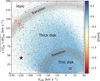 |
Fig. 1 Toomre diagram showing HE2159-0551 (red star). The Sun is indicated with a red circle. The dotted lines represent contours of constant total space velocity, υtot. Stars from the GALAH background sample (Buder et al. 2024) with [Fe/H] < −2.00 dex are highlighted. |
5.3 Investigating the origin of HE2159-0551
To further examine the origin of HE2159-0551, we analyzed its position in the E-Lz plane. Because orbital energy and the z-component of angular momentum are integrals of motion, stars originating from the same accretion event naturally share similar values of these quantities, even when scattered throughout the Galaxy (e.g., Helmi & de Zeeuw 2000; Gómez et al. 2010; Simpson et al. 2019). As a first approximation, we used the identification of the substructures in the stellar halo, as stated in Naidu et al. (2020) and Horta et al. (2022). Using the previously calculated orbital parameters for HE2159-0551 and the background stars (see Sect. 5.1), we plotted the E-Lz plane in Fig. 2 (left). We note that HE2159-0551 fits in the following selection criteria for the LMS-1/Wukong8 merger from Horta et al. (2022): 0.20 < Lz < 1 [103 kpc km s−1 ], −1.70 < E < −1.20 [105 km2 s−2], and [Fe/H] < −1.45 dex, 0.40 < ⏋ < 0.70, and |Z| > 3 [kpc]. Adopting the selection criteria from Horta et al. (2022), we identified 62 LMS-1/Wukong stars in our background sample.
LMS-1 is a stellar substructure that was recently discovered by Yuan et al. (2020). It comprises MP stars that manifest themselves as an overdensity close to the lower edge of the Gaia-Enceladus/Sausage (GES) merger in the E-Lz plane. This population was subsequently analyzed in detail by Naidu et al. (2020), who named it Wukong and highlighted its slightly pro-grade orbital motion in a polar orientation. Malhan (2022) conclude that it represents the most MP accretion event identified so far in the Milky Way, characterized by a metallicity distribution function (MDF) extending down to [Fe/H] ≈ −3.40 dex. Limberg et al. (2024) further refined the dynamical characterization of LMS-1/Wukong. Combining kinematics and abundances, we find a chemodynamical selection important and stick to the definition from Horta et al. (2022). Based on the Mg and Fe abundances and the overlap in the E-Lz plane of LMS-1/Wukong and the Helmi-Stream, it is possible that these two substructures could be linked, where LMS-1/Wukong constitutes the more MP component of the Helmi-Stream. However, Naidu et al. (2020) suggest that it is an independent substructure based on the metallicity peak in the MDF of the stars, including their definition in the E-Lz plane. In addition to Naidu et al. (2020) and Horta et al. (2022), we also show an alternative selection for LMS-1/Wukong, based on unpublished criteria from Monty et al. (in prep.), indicated by the dashed ellipse in Fig. 2. This region encloses the typical locus of their LMS-1/Wukong candidates in the E-Lz space and is manually defined to capture their dynamical clustering.
Several extremely MP stellar streams have since been linked to LMS-1/Wukong. In particular, the streams C19 ([Fe/H] = −3.38 ± 0.06 dex; Martin et al. 2022), Sylgr ([Fe/H] = −2.92 ± 0.06 dex; Roederer & Gnedin 2019), and Phoenix ([Fe/H] = −2.70 ± 0.06 dex; Wan et al. 2020) are identified as belonging to this merger. Additionally, the stellar streams Indus and Jhelum have been preliminarily proposed to be associated with LMS-1/Wukong by Bonaca et al. (2021). While the association of Indus with LMS-1/Wukong is further supported by Malhan et al. (2021), the same study casts doubt on Jhelum’s membership. Considering that both Indus and Jhelum are debris of disrupted dwarf galaxies (Li et al. 2022), it appears likely that they were satellite dwarf companions orbiting the progenitor galaxy of LMS-1/Wukong (also see Malhan et al. 2021). This evidence suggests that LMS-1/Wukong originated from a particularly ancient and MP dwarf galaxy that formed at an early epoch of galaxy formation. According to dynamical analyses by Malhan et al. (2021), the LMS-1 progenitor was likely accreted onto the Milky Way at least ≳8–10 Gyr ago.
In the action diamond (Fig. 2, right), HE2159-0551 is clearly located near stars identified as members of LMS-1/Wukong. This visualization emphasizes orbital characteristics such as radiality and angular momentum components, which are particularly useful for distinguishing accreted populations from stars formed in situ within the Milky Way. Interestingly, HE2159-0551 exhibits a distinctly prograde orbital signature compared to the main body of LMS-1/Wukong stars, suggesting a unique dynamical history. Such a prograde orbit typically characterizes stellar populations of the Galactic thick disk, indicating that HE2159-0551 may represent a special case of an LMS-1/Wukong star that has dynamically migrated toward thick-disk orbital properties. We note that two additional MP stars have been discovered in an independent study by Monty et al. (in prep.), which also seem to belong to LMS-1/Wukong.
This scenario implies the existence of a previously unrecognized transition region or overlap zone between the LMS-1/Wukong merger debris and the thick-disk component of the Galaxy, potentially created through dynamical mixing processes such as disk heating or radial migration. Furthermore, the position of HE2159-0551 in this orbital parameter space raises the question of possible overlaps or transitions between LMS-1/Wukong and other known substructures, notably the Helmi stream. To address this possibility, we applied the orbital definition of the Helmi stream from Koppelman et al. (2019b), namely 0.70 < Lz < 1 [103 kpc km s−1] and 1.60 < L⊥9 < 3.20 kpc km s−1, to test for membership. Our analysis reveals that HE2159-0551 does not fulfill these Helmi stream criteria. Thus, despite the apparent dynamical proximity, the star can be firmly excluded as a Helmi stream member. This reinforces the interpretation that HE2159-0551 represents an intriguing transitional object situated in a kinematical overlap region connecting the LMS-1/Wukong merger event with the Milky Way’s thick disk, rather than bridging to the Helmi stream. This finding highlights the complexity of stellar orbital histories and the importance of precise chemodynamical analyses to fully disentangle Galactic substructures. Such findings reinforce the importance of LMS-1/Wukong as a crucial tracer for investigating galaxy formation and early nucleosynthesis.
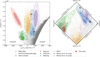 |
Fig. 2 Orbital properties of HE2159-0551 (red star) compared to known stellar substructures in the Milky Way. Left: E–Lz diagram showing orbital energy vs. angular momentum. Colored points and contours (based on a Gaussian density distribution) indicate the location of accreted populations from the literature. Specifically, GES (Belokurov et al. 2018; Helmi et al. 2018), Sequoia (Myeong et al. 2019), Thamnos (Koppelman et al. 2019a), Helmi stream (Helmi et al. 1999), LMS-1 (Yuan et al. 2020), and Wukong (Naidu et al. 2020) are shown. HE2159-0551 lies within the Wukong selection region, but at the prograde edge of the structure. Right: action diamond diagram with x = Jϕ/Jtot and y = (Jz – JR)/Jtot, where Jtot = JR + |Jϕ| + Jz. HE2159-0551 again appears within the Wukong region. |
Overview of derived abundances and uncertainties (σ) organized by atomic number.
6 Chemical abundances
We utilized the software PyMoogi and its synthesis driver to derive chemical abundances or place limits (indicated as []) on 23 elements: C, N, [O], Na, Mg, [Al, Si], K, Ca, Sc, Ti, V, Cr, [Mn], Fe, Co, Ni, Zn, [Sr], Y, Zr, Ba, and [Eu] (see Table 4 and Figs. 3 to 6). We conducted a visual comparison between the observed and synthetic spectra, striving to minimize the standard deviation to achieve the closest possible match between the two spectra. We determined the Fe abundance using EWs, ensuring that the spectral lines were clean. To validate our results, we then performed spectral synthesis of Fe. Line lists are generated using Linemake10 (Placco et al. 2021). We calculated the uncertainty for all elemental abundances by changing the stellar parameters one by one by their attributed uncertainty, while acknowledging that statistical errors could also arise from factors such as continuum placement.
The derived chemical abundances are provided in Table 4 and are scaled to the solar abundances of Asplund et al. (2009). In Fig. 3 we present all derived abundances and limits including the uncertainties of each individual element in comparison to the results for HE2159-0551 by Hansen et al. (2015, 2018b), CS22892-052 (Sneden et al. 2003), and HD 122563 (Honda et al. 2006, 2004). In Fig. 4 we provide examples of individual synthesized lines for six different elements (Sr, Ba, Eu, Sc, Zr, and Co). Figures 5 and 6 provide comparisons of specific element abundances to literature data from the CERES (Chemical Evolution of R-process Elements in Stars) project (Lombardo et al. 2022, 2025; de Melo et al. 2024) and the GALAH sample (Buder et al. 2024).
We combined spectra from different observing nights to enhance the spectral S/N compared to earlier studies. The abundances derived in Hansen et al. (2015, 2018b) are listed in Table 5 and illustrated in Fig. 3 together with the abundances from this study. A comparison of the two papers reveals small differences in their derived abundances, which is also reflected in their metallicity values: −2.81 dex in Hansen et al. (2015) and −2.75 dex in Hansen et al. (2018b). Overall, most abundances from the literature of Hansen et al. (2015, 2018b) agree with our results within combined uncertainties, indicating strong consistency and reliability across studies. However, different lines can be sensitive to varying conditions (e.g., Fe II lines being more gravity-sensitive than Fe I lines), leading to some discrepancies. A careful selection of lines is crucial and can account for discrepancies when comparing to literature values.
We also attempted to derive abundances or place limits for other elements: Li, Be, S, Cu, Rb, Mo, Ru, Pd, Ag, La, Ce, Pr, Sm, Gd, Dy, Ho, Er, Os, Pt, Pb, Th, and U (see also Sect. 7). Unfortunately, these attempts were unsuccessful. The primary reason is that the spectral features for these elements are extremely weak and in many cases no discernible line is present. The expected position of the lines do not exhibit any signal distinguishable from the spectral noise, precluding the possibility of reliably measuring abundances or even setting limits. The noise dominates the relevant spectral regions and any feature that might correspond to a heavy-element line is completely buried. This likely has its ties in the peculiar nucleosynthesis event that enriched the star partially and in too low levels of most heavy elements. As an illustrative example, Fig. 7 shows the expected position of the Gd line in the blue region of the spectrum, highlighting the absence of a detectable line. This plot is representative of the spectral appearance of the heavy elements throughout the spectra.
Furthermore, we compared our seemingly r-peculiar star to two other well-known stars: CS22892-052 (r-rich; Sneden et al. (2003)) and HD 122563 (r-poor; Honda et al. (2006, 2004)) in Fig. 3. Both studies provide a comprehensive range of abundances for the individual VMP stars. Notably, the abundances of heavier elements vary among the three stars. HE2159-0551 aligns more closely with the star HD 122563 considering that we find no detection for elements with Z > 56.
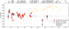 |
Fig. 3 [X/Fe] versus atomic number Z for HE2159-0551 (this work: red stars) with uncertainties. Data points with a downward or upward facing arrow represent upper or lower limits, respectively. HE2159-0551 is compared to Hansen et al. (2015, black), Hansen et al. (2018b, blue), CS22892-052 (Sneden et al. 2003, orange), and HD 122563 (Honda et al. 2004, 2006, gray). The horizontal dotted line shows [X/Fe] = 0.00 dex. |
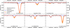 |
Fig. 4 Top: line synthesis of Sr, Ba, and Eu with the best fit indicated in red: [Sr/Fe] ≥ −0.01 dex (saturated), [Ba/Fe] = −0.84 dex, and [Eu/Fe] ≤ −0.02 dex (noisy). Bottom: [Sc/Fe] = 0.02 dex, [Zr/Fe] = 0.39 dex, and [Co/Fe] = 0.16 dex. Uncertainties are shaded in yellow and observed spectra in black. Continuum is shown in gray, while a blue line denotes the absence of the element measured. |
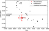 |
Fig. 5 [C/N] versus temperature of HE2159-0551 (red) in comparison to the CERES project stars (de Melo et al. 2024, black), distinguishing between mixed (below the gray line) and unmixed (above the gray line) stars. |
Abundances and uncertainties derived in this study compared to the literature values of Hansen et al. (2015, (1)) and Hansen et al. (2018b, (2)).
6.1 Carbon, nitrogen, and oxygen
We derived abundances for C and N using the CH and NH molecular bands, yielding [C/Fe] = −0.10 ± 0.33 dex and [N/Fe] = 0.75 ± 0.25 dex. The star is N-enhanced, but not C-enhanced, following the criteria of Beers & Christlieb (2005) and Aoki et al. (2007), who define carbon-enhanced MP (CEMP) stars as [C/Fe] > +0.70 dex. The measured [C/N] = −0.85 dex indicates that mixing has occurred; see Fig. 5. Hence, mixing processes have affected the star’s lighter element abundances (e.g., Spite et al. 2005). Placco et al. (2014) provide a correction11 accounting for C depletion due to mixing. Our [N/H] deviates from solar, rendering these corrections inaccurate. We find [O/Fe] ≤ 0.68 ± 0.41 dex. Our C and N abundances agree within uncertainties when comparing to Hansen et al. (2015), who use molecular bands around 4300 Å, 3360 Å, 3890 Å, and 4215 Å, mostly consistent with those used in this work (see Table 4).
6.2 Sodium, aluminum, chromium, scandium, and manganese
We determine [Na/Fe] = −0.34 ± 0.25 dex. We also inspected the Na lines at 5889.95 Å and 5895.95 Å. Due to saturation issues, we neglected the abundance of those lines when determining the final mean Na abundance value. The A1 line yields a lower limit (LL) of [A1/Fe] ≥ −0.85 ± 0.44 dex, as we had to rely on a blended, saturated line. While Baumüller & Gehren (1997) report near-solar [A1/Fe] ratios in VMP stars, our value is lower, but falls within the observed scatter around [Fe/H] ≈ −2.60 dex, which they attribute to NLTE effects. We find [Cr/Fe] = −0.23 ± 0.08 dex, consistent with the MP average in François et al. (2004). We determine [Sc/Fe] = 0.02 ± 0.06 dex, which shows less enhancement, consistent with expectations for MP stars (Cayrel et al. 2004; Frebel 2008; Hayek et al. 2009; Hansen 2011). For Mn, we find a limit of [Mn/Fe] ≥ −0.50 ± 0.20 dex from blended, but also saturated lines. Despite the large uncertainty, the result is in line with the studies by Gratton (1989) and Sobeck et al. (2006), who report subsolar Mn abundances decreasing with decreasing metallicity. However, near [Fe/H] ≈ −2.00 dex, they observe an increase in the Mn abundance. HE2159-0551 seems to follow this trend. To probe the star’s origin, we computed [Mg/Mn] ≤ 0.86 dex, see Sect. 6.7.
6.3 Magnesium, silicon, calcium, and titanium
We derive [Mg/Fe] = 0.36 ± 0.11 dex, [Ca/Fe] = 0.23 ± 0.13 dex, and [Ti/Fe] = 0.33 ± 0.07 dex. We placed an LL of [Si/Fe] = ≥ 0.29 ± 0.23 dex due to saturation issues. The Mg, Si, and Ti enhancements (≈ 0.35 dex) are typical for VMP stars and reflect early α-element enrichment from Type II SNe during the galaxy’s early chemical evolution. Our derived Mg, Si, and Ti abundances are consistent within uncertainties when comparing with Hansen et al. (2015). The Ca abundance is slightly higher but still compatible. This is in line with the Ca values derived in Sagittarius (Sgr) in VMP and extremely MP stars (Hansen et al. 2018a).
Based on [C/Mg] = −0.46 dex, we classify the star as multi-enriched, implying enrichment from multiple nucleosynthetic events (Hartwig et al. 2018). This is consistent with our expectations, although such classifications are subject to uncertainties from gas dilution, mixing, and variations in progenitor properties of SNe (Hansen et al. 2020).
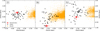 |
Fig. 6 Comparison of HE2159-0551 (this work, red), the CERES project sample (Lombardo et al. 2022, 2025, black), and the GALAH sample (Buder et al. 2024, orange), also used in Sect. 5. |
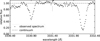 |
Fig. 7 Non-detection of Gd. The perpendicular gray line indicates the wavelength of Gd at 3331.40 Å and shows that no abundance and/or limit can be derived and/or placed for this element. |
6.4 Potassium, vanadium, cobalt, nickel, and zinc
We derive [K/Fe] = 0.58 ± 0.20 dex, [V/Fe] = 0.15 ± 0.26 dex, [Co/Fe] = 0.16 ± 0.23 dex, [Ni/Fe] = 0.06 ± 0.23 dex, and [Zn/Fe] = 0.34 ± 0.07 dex, consistent with results of other stars in Da Silveira et al. (2018), who report Zn behaving similarly to α-elements. While Zn shows scatter near solar metallicity (Duffau et al. 2017), elevated [Zn/Fe] ratios are attributed to SN enrichment (Da Silveira et al. 2018, and references therein). At [Fe/H] ≈ −3.00 dex, Zn abundances in the Milky Way halo can reach supersolar abundances of [Zn/Fe] ≈ 0.50 dex (Duffau et al. 2017), placing our result within the expected range given the uncertainties. The abundance results of this subsection agree within combined uncertainties when compared to Hansen et al. (2015).
6.5 Strontium, yttrium, zirconium, and barium
We attempted to determine the Sr abundance using the 4077.71 Å and 4215.52 Å lines. However, due to the strong and saturated lines, we report an LL of [Sr/Fe] ≥ −0.01 ± 0.20 dex. The weaker Sr line at 4607.33 Å is not covered by our spectra. Although we used the same lines as Hansen et al. (2015), our derived abundance is lower. In contrast, Hansen et al. (2018b) primarily used the 4215.52 Å line due to similar saturation issues. Hansen et al. (2012) report a mean abundance of [Sr/Fe] ≈ 0.14 dex down to [Fe/H] = −2.50 dex in a larger MP sample, with increased scatter at lower metallicities - our result lies well within this scatter.
We derive [Y/Fe] = −0.18 ± 0.11 dex, [Zr/Fe] = 0.39 ± 0.07 dex, and [Ba/Fe] = −0.84 ± 0.12 dex. The spread of more than 1.20 dex between these element abundances is notable. Y and Zr are primarily s-process elements, with contributions of 77.80% and 81.70%, respectively (Prantzos et al. 2020)12; however, at low metallicities around [Fe/H] = −2.40 dex and below, the production of these elements is influenced by the limited presence of AGB stars, as well as contributions from other stellar processes (Simmerer et al. 2004; Lombardo et al. 2025). Hansen et al. (2012) suggest Zr may originate from both the weak r- and main s-process, reporting a mean [Zr/Fe] ≈ 0.20 dex for [Fe/H] ≥ −2.50 dex, but with increasing scatter at lower metallicities, consistent with our results. The Y and Zr abundances agree with those in Mello et al. (2014), Lombardo et al. (2022), and François et al. (2007) for stars of similar metallicity. The elevated Zr and low Y might be explained by SN enrichment or the νp-process, as internal stellar mixing appears to have little or no effect on Sr, Y, and Zr abundances (de Melo et al. 2024).
Barium is mainly formed by the s-process in AGB stars. The low Ba abundance combined with the solar-scaled Y, however, makes AGB stars an unlikely formation site (see also Appendix D). Our Ba abundance follows the trend of MP stars (Lombardo et al. 2022, 2025) (see Fig. 6). The large Ba scatter at [Fe/H] < −2.50 dex, also seen in the sample of Hansen et al. (2012) and François et al. (2007), may reflect poor interstellar medium (ISM) mixing or cosmic variations (Barklem et al. 2005; François et al. 2007), warranting further investigation with additional sample stars. Ba abundances of HE2159-0551 vary across studies of Hansen et al. (2015) and Hansen et al. (2018b), but our results agree well with Hansen et al. (2018b), who use the same lines as we do (5853.70 Å, 6141.70 Å, and 6496.90 Å). This low Ba abundance agrees with the weak r-or νp-process forming Sr-Zr but not reaching Ba. This could be associated with an intermediate or massive SN producing Ca to Zr, but not Ba or heavier. We speculate that the low Ba abundance we find in this star might be attributed to the LMS-1/Wukong merger event, as the kinematical analysis of this star indicates that it originated from this merger event (see Sect. 5.3). This highlights the significance for investigating stars chemody-namically and taking all properties into consideration. The low Ba abundance for LMS-1 candidates has been derived in two other stars in an independent study by Monty et al. (in prep.) and may be a tracer for LMS-1.
6.6 Heavy element upper limits
We place an upper limit (UL) of [Eu/Fe] ≤ −0.02 ± 0.16 dex, based on a weak line affected by significant noise. As Eu is 95.10% r-process produced, the low abundance is noteworthy for a VMP star. Compared to the CERES stars (Lombardo et al. 2025) and the GALAH sample (Buder et al. 2024), our target only marginally follows the trend of decreasing Eu with metallicity and lies outside the main distribution in Fig. 6, suggesting a lack of r-process and overall n-capture enhancement. The result is consistent with that from Hansen et al. (2015, 2018b). While surface abundances may be affected by mixing, elements like Sr, Y, and Zr are not expected to show such noteworthy effects (de Melo et al. 2024), supporting the interpretation that [Ba/Eu] reflects the star’s initial composition.
Based on the heavy element abundances and/or limits, we find no strong s- or r-process enhancement. A type of weak n-capture or vp-process may have enriched this star, which explains the elemental abundances up to Zr and a low abundance of Ba. The heavier limit supports the result of (multi-)enrichment of an ISM that was mixed poorly and had a low abundance of Ba and Eu, consistent with multi-enrichment, likely from the weak r-/νp-process following an SN II.
6.7 Abundance planes
Our goal is to determine whether HE2159-0551 formed in situ or was accreted into the Galaxy. In principle, abundance planes such as [Mg/Fe] versus [Fe/H], [C+N/Fe] versus [Fe/H], [Al/Fe] versus [Fe/H], and particularly [Mg/Mn] versus [Al/Fe] have been successfully used to distinguish between accreted and in situ stellar populations (Freeman & Bland-Hawthorn 2002; Tolstoy et al. 2009; Hawkins et al. 2015; Das et al. 2020). [Mg/Mn] is used to highlight the α-poor population rather than [Mg/Fe], as Mn is a pristine tracer of SN Ia. Moreover, since SN Ia do not produce A1 as efficiently as Fe, the [A1/Fe] plane can be used to distinguish accreted stars born in less massive systems, whereas in situ stars display elevated [A1/Fe] and lower [Mg/Mn] values.
Unfortunately, in the case of HE2159-0551, we can only place limits for abundances of key diagnostic elements such as A1 and Mn. Due to these constraints, the star’s position in these abundance diagrams is uncertain and provides only limited diagnostic power. Although our placed UL on [A1/Fe] and LL on [Mg/Mn] would, in principle, support an accreted origin, the lack of precise abundances makes such conclusions tentative. For this reason, we refrain from explicitly presenting these abundance planes. Nonetheless, we emphasize that we carefully inspected these chemical signatures and find that the overall chemodynamical evidence, particularly the orbital parameters consistent with LMS-1 membership, remains compelling. Thus, despite the limited diagnostic value from abundances of A1 and Mn, we maintain our interpretation of HE2159-0551 as an exceptional LMS-1 star, dynamically mixed into a thick-disk region of the Galaxy.
7 Discussion and conclusion
We present kinematics and more abundance measurements for the star HE2159-0551 than previously reported in the literature, revealing a peculiar abundance pattern and a connection to the LMS-1/Wukong merger event. Our results show good overall agreement with the stellar parameters and abundances of Hansen et al. (2015, 2018b). Accurate determination of these parameters is crucial, as uncertainties in stellar parameters can influence abundance results by several tenths of a dex.
By utilizing spectra collected over several years, we are able to improve both the reliability and S/N of our data, as well as refute binarity. A complete set of clean lines and accurate atomic physics (excitation potential and oscillator strengths) ensure that the abundance estimates are not biased by noise or uncertainties in individual measurements.
In addition to the elements mentioned above, we also attempted to derive abundances for Li, Be, S, Cu, Rb, Mo, Ru, Pd, Ag, La, Ce, Pr, Sm, Gd, Dy, Ho, Er, Os, Pt, Pb, Th, and U. Unfortunately, the abundances of these elements could not be determined due to the presence of very weak or nonexistent spectral lines (see Sect. 6) in the spectra with S/N of about 70 at 4000 Å and 100 at 5000 Å. The inability to measure Li is particularly notable, as it suggests significant depletion of Li in this VMP star – consistent with the findings of Korn et al. (2006) – confirming internal mixing. The internal mixing processes related to the red giant branch bump alter the surface abundances of certain lighter elements, but cannot explain the anomalies observed in the heavier elements (de Melo et al. 2024, and references therein). The low Ba reflects more complex nucleosynthesis processes at play prior to the star’s formation.
The scatter observed in the abundances of elements such as Sr, Y, Zr, Ba, and Eu at [Fe/H] < −2.50 dex is often interpreted as a consequence of poor mixing in the ISM due to a limited number of SNe (Hansen et al. 2012, 2014). This scatter implies that the star’s chemical composition was shaped by only a few nucleosynthetic events, reinforcing the idea that HE2159-0551 may have experienced an unusual enrichment history. A key feature of this star is its low abundances of n-capture elements, including Y and especially Ba. This suggests that the star has not undergone a third dredge-up event, nor has it been pre-enriched in s-process elements, distinguishing it from many other stars of similar metallicity. This unique characteristic points to a potentially distinct nucleosynthesis history for the star, which may be connected to the LMS-1/Wukong merger. This galaxy might exhibit a peculiar and generally low Ba abundance at low metallicity as chemical tracers.
In typical r-process-enhanced VMP stars, higher element abundances tend to resemble solar values (Barklem et al. 2005); however, this star’s deviation suggests a completely different nucleosynthetic history. Numerous studies in the literature have identified stars exhibiting exceptionally low abundances of heavy elements (e.g., Koch et al. 2008, 2013; Fulbright et al. 2004). In each of these cases, the prevailing interpretation suggests that the observed enrichment of heavy elements is primarily the result of contributions from a limited number of very massive stars. Considering that the star HE2159-0551 is associated with the LMS-1/Wukong merger event, it is reasonable to attribute the divergent nucleosynthesis processes to this connection. The weak r- or νp-process in an SN explosion may have contributed to the early ISM of LMS-1/Wukong, but the conditions were too proton (or neutrino) rich to efficiently form elements much heavier than Zr. Consequently, there is no strong r-enrichment from NSMs at [Fe/H] ~ −2.50 dex; otherwise, we would expect a higher abundance level of Eu in this star.
The LMS-1/Wukong system was probably enriched primarily by a few normal, low-mass CC SN, which could facilitate, for example, a νp-process that forms Sr-Zr, but does not produce Ba in significant quantities more than 10 Gyr ago – prior to the merger event. The galaxy merger event may have triggered additional SN explosions and star formation. The material from these SNe would have mixed within the LMS-1/Wukong system, which exhibits only a low level of r-process elements, possibly originating from the mini-halo stages. It is only above [Fe/H]~ − 2.50 dex that NSMs would significantly enrich the LMS-1/Wukong system. This observation provides a promising constraint on the compact merger delay times, placing the LMS-1/Wukong system as a counterpart to the ultra-faint dwarfgalaxy Reticulum II, which exhibits high levels of heavy n-capture abundances at low metallicities (Ji et al. 2016).
Jean-Baptiste et al. (2017) showed that a single accretion event can lead to multiple overdensities in orbital space (see also Koppelman et al. 2020). An association between LMS-1 and Wukong seems plausible due to their close proximity in orbital planes (see Fig. 2) and the chemical similarity, in particular the low Ba abundance which we and Monty et al. (in prep.) individually find (see Sect. 6.5). This suggests that they are indeed the same system, which exhibits peculiar abundances at low metallicity. However, we defer providing a definitive conclusion until more elemental abundances are obtained in a larger sample of both LMS-1 and Wukong candidates.
Acknowledgements
Based on observations collected at the European Organisation for Astronomical Research in the Southern Hemisphere under ESO programmes 095.D-0402(A) and 077.D-0035(A) and on data obtained from the ESO Science Archive Facility. This work has made use of data from the European Space Agency (ESA) mission Gaia (https://www.cosmos.esa.int/gaia), processed by the Gaia Data Processing and Analysis Consortium (DPAC, https://www.cosmos.esa.int/web/gaia/dpac/consortium). Funding for the DPAC has been provided by national institutions, in particular the institutions participating in the Gaia Multilateral Agreement. NOIRLab IRAF is distributed by the Community Science and Data Center at NSF NOIRLab, which is managed by the Association of Universities for Research in Astronomy (AURA) under a cooperative agreement with the U.S. National Science Foundation. AS acknowledges the support by the State of Hesse within the Research Cluster ELEMENTS (Project ID 500/10.006). AS was supported by the Deutsche Forschungsgemeinschaft (DFG, German Research Foundation) - Project-ID 279384907 - SFB 1245. CJH acknowledges ChETEC-INFRA (EU project no. 101008324) and HFHF. AS acknowledges the helpful input of Linda Lombardo, Raphaela Fernandes de Melo, Arthur Alencastro Puls, Alexander Dimoff, Andrew Gallagher, and Andreas Koch-Hansen. We thank the referee for constructive feedback. Finally, we acknowledge fruitful discussions with S. Monty and J. Bovy. Software: Astropy (Astropy Collaboration 2013, 2018, 2022), Numpy (Harris et al. 2020), SciPy (Virtanen et al. 2020), Matplotlib (Hunter 2007), Galpy (Bovy 2015).
Appendix A Radial velocity
In Table A.1 we present a detailed overview of the computed RVs discussed in Sect. 3.
Computed RV values (single-file (shifting) and CC method) including computed BC, separated by individual observations with information on exposure time, slit width, central wavelength, and S/N for each file.
Appendix B Stellar parameters – uncertainties
We use the following assumptions for the computation of the uncertainties of the stellar parameters: we compute the effective temperature as 5000 K, with additional models ± 100 K, while keeping the other stellar parameters fixed. Similarly, we assess models for the surface gravity; the final value of 1.80 dex ± 0.20 dex. For the microturbulence, with a computed value of 2.40 km s−1, we create models with± 0.20 km s−1. Using the outputs from these models, we compute uncertainties by analyzing the slope changes of the Fe I lines in response to variations in the individual parameters. We then quantify the uncertainty by computing the difference between the original value and the values from the modified models. We present the computation for log g here and apply the same procedure to the other two stellar parameters:
 (B.1)
(B.1)
 (B.2)
(B.2)
We compute the average difference in slopes by calculating:
 (B.3)
(B.3)
This leads to the uncertainty of e.g., the surface gravity:
 (B.4)
(B.4)
With this, we get an uncertainty of 0.40 dex for log g. Following the same procedure for vt leads to an uncertainty of0.30 km s−1.
For the uncertainty in temperature, the slope change is a critical factor. Aslopechangeof0.001 for the Fe I lines corresponds to a variation in effective temperature of 3.22 K when the slope increases, and 2.32 K when it decreases. Thus, for simplicity we assume that a slope change of 0.001 results in an approximate temperature variation of 3 K. This allows us to compute the final uncertainty in temperature by considering the average slope difference for log g = 0.03, for vt = 0.02, and for Teff = 0.03 when comparing the computed models to the modified models. We find the uncertainty for Teff and log g as 90 K13 and for vt as 60 K14 by using the relation 3 K/0.001 = 3000 K/slope. Therefore, the uncertainty in the effective temperature is
 (B.5)
(B.5)
 (B.6)
(B.6)
The actual temperature uncertainty could be expressed as ± 90 K (rounded to ± 100 K). However, this estimate does not account for the interdependencies among the stellar parameters. To incorporate these dependencies, we refer to equation B.5 and report the final uncertainty value for the effective temperature as ± 140 K.
Appendix C Kinematics
We list the 6D phase-space values and their uncertainties, used in Sect. 5, in Table C.1.
6D phase-space values and their uncertainties for HE2159-0551’s orbit and orbital parameters.
Appendix D Nucleosynthesis models
We use the F.R.U.I.T.Y. database (Cristallo et al. 2011) to compare our abundance measurements with synthetic models of AGB stars. For our models, we assume an initial rotational velocity of zero and adopt the standard configuration for 13C pockets. We systematically vary the mass of the AGB stars while fixing the metallicity at Z = 0.00005 and set [α/Fe] = 0.50 dex. This metallicity corresponds to [Fe/H] ≃ −2.40 dex, which is the closest available value in the F.R.U.I.T.Y. database to our computed metallicity in Sect. 4: [Fe/H] ≃ −2.60 dex, Z = 0.0000682093. The conversion follows the relation Z = Zsolar ⋅ 10[Z/H], where we adopt a solar metallicity of Zsolar = 0.013 based on Grevesse et al. (2012). Additionally, we generate models for the same mass range at an even lower metallicity of Z = 0.00002, [α/Fe] = 0.50 dex, corresponding to [Fe/H] ≃ −2.81 dex. We present the resulting plot in Fig. D.1.
Our analysis suggests that the models do not match any current nucleosynthesis model, indicating that AGB stars cannot explain the observed abundance pattern. The lower abundance of Ba suggests a lack of significant AGB star enrichment, consistent with expectations for low-metallicity stars or environments with minimal s-process contribution, which we can confirm when comparing to the model.
By comparing all observed abundances to the F.R.U.I.T.Y models, we can conclude that additional stellar sources or nucle-osynthetic processes may have played a role in shaping the chemical composition of this star. Potential contributors include e.g., rotating massive stars (Frischknecht et al. 2012), i-process nucleosynthesis, νp-process, NSMs, or CC SNe, each of which could have played a role in shaping the chemical enrichment of this star.
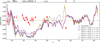 |
Fig. D.1 F.R.U.I.T.Y. models (Cristallo et al. 2011) in comparison to the derived abundances of HE2159-0551 (red stars). The upper and lower limits are represented as downward and upward facing arrows, respectively. The different colors represent different masses and metallicities. The horizontal dotted line shows [X/Fe] = 0.00 dex. For all models, we assume [α/Fe] = 0.50 dex and set [Y/Fe] = 0.00 dex. |
References
- Abbott, B. P., Abbott, R., Abbott, T. D., et al. 2017, Phys. Rev. Lett., 119, 161101 [Google Scholar]
- Aguado, D. S., Belokurov, V., Myeong, G. C., et al. 2021, ApJ, 908, L8 [NASA ADS] [CrossRef] [Google Scholar]
- Alencastro Puls, A. 2023, PhD thesis [Google Scholar]
- Aoki, W., Beers, T. C., Christlieb, N., et al. 2007, ApJ, 655, 492 [NASA ADS] [CrossRef] [Google Scholar]
- Arcones, A., & Bliss, J. 2014, J. Phys. G: Nucl. Part. Phys., 41, 044005 [Google Scholar]
- Arcones, A., & Thielemann, F.-K. 2023, A&AR, 31, 1 [NASA ADS] [CrossRef] [Google Scholar]
- Asplund, M., Grevesse, N., Sauval, A. J., & Scott, P. 2009, ARA&A, 47, 481 [NASA ADS] [CrossRef] [Google Scholar]
- Astropy Collaboration (Robitaille, T. P., et al.) 2013, A&A, 558, A33 [NASA ADS] [CrossRef] [EDP Sciences] [Google Scholar]
- Astropy Collaboration (Price-Whelan, A. M., et al.) 2018, AJ, 156, 123 [Google Scholar]
- Astropy Collaboration (Price-Whelan, A. M., et al.) 2022, ApJ, 935, 167 [NASA ADS] [CrossRef] [Google Scholar]
- Bailer-Jones, C. A. L., Rybizki, J., Fouesneau, M., Demleitner, M., & Andrae, R. 2021, VizieR Online Data Catalog: Distances to 1.47 billion stars in Gaia EDR3 (Bailer-Jones+, 2021), VizieR On-line Data Catalog: I/352. Originally published in: 2021AJ….161..147B [Google Scholar]
- Barklem, P. S., Christlieb, N., Beers, T. C., et al. 2005, A&A, 439, 129 [NASA ADS] [CrossRef] [EDP Sciences] [Google Scholar]
- Baumüller, D., & Gehren, T. 1997, A&A, 325, 1088 [Google Scholar]
- Beers, T. C., & Christlieb, N. 2005, ARA&A, 43, 531 [NASA ADS] [CrossRef] [Google Scholar]
- Belmonte, M., Pickering, J., Ruffoni, M., et al. 2017, ApJ, 848, 125 [NASA ADS] [CrossRef] [Google Scholar]
- Belokurov, V., Erkal, D., Evans, N. W., Koposov, S. E., & Deason, A. J. 2018, MNRAS, 478, 611 [Google Scholar]
- Bennett, M., & Bovy, J. 2018, MNRAS, 482, 1417 [Google Scholar]
- Bensby, Feltzing, S., & Lundström, I. 2003, A&A, 410, 527 [CrossRef] [EDP Sciences] [Google Scholar]
- Bensby, Feltzing, S., & Oey, M. S. 2014, A&A, 562, A71 [NASA ADS] [CrossRef] [EDP Sciences] [Google Scholar]
- Bergemann, M., Lind, K., Collet, R., & Asplund, M. 2011, in J. Phys. Conf. Ser., 328, Journal of Physics Conference Series, 012002 [NASA ADS] [CrossRef] [Google Scholar]
- Bergemann, M., Lind, K., Collet, R., Magic, Z., & Asplund, M. 2012, MNRAS, 427, 27 [Google Scholar]
- Bergeson, S. D., & Lawler, J. 1993, ApJ, 408, 382 [Google Scholar]
- Biémont, É., Blagoev, K., Engström, L., et al. 2011, MNRAS, 414, 3350 [Google Scholar]
- Blanton, M. R., Bershady, M. A., Abolfathi, B., et al. 2017, AJ, 154, 28 [Google Scholar]
- Bonaca, A., Naidu, R. P., Conroy, C., et al. 2021, ApJ, 909, L26 [NASA ADS] [CrossRef] [Google Scholar]
- Bovy, J. 2015, ApJS, 216, 29 [NASA ADS] [CrossRef] [Google Scholar]
- Buder, S., Kos, J., Wang, E. X., et al. 2024, The GALAH Survey: Data Release 4 [Google Scholar]
- Burbidge, E. M., Burbidge, G. R., Fowler, W. A., & Hoyle, F. 1957, RMP, 29, 547 [Google Scholar]
- Castelli, F., & Kurucz, R. L. 2003, in IAU Symposium, 210, Modelling of Stellar Atmospheres, eds. N. Piskunov, W. W. Weiss, & D. F. Gray, A20 [NASA ADS] [Google Scholar]
- Cayrel, R., Depagne, E., Spite, M., et al. 2004, A&A, 416, 1117 [NASA ADS] [CrossRef] [EDP Sciences] [Google Scholar]
- Christlieb, N., Beers, T. C., Barklem, P. S., et al. 2004, A&A, 428, 1027 [NASA ADS] [CrossRef] [EDP Sciences] [Google Scholar]
- Cowan, J. J., Sneden, C., Lawler, J. E., et al. 2021, RMP, 93, 015002 [CrossRef] [Google Scholar]
- Cristallo, S., Piersanti, L., Straniero, O., et al. 2011, ApJS, 197, 17 [NASA ADS] [CrossRef] [Google Scholar]
- Da Silveira, C., Barbuy, B., Friaça, A. C. S., et al. 2018, A&A, 614, A149 [NASA ADS] [CrossRef] [EDP Sciences] [Google Scholar]
- Das, P., Hawkins, K., & Jofré, P. 2020, MNRAS, 493, 5195 [NASA ADS] [CrossRef] [Google Scholar]
- de Melo, R. F., Lombardo, L., Puls, A. A., et al. 2024, A&A, 691, A220 [NASA ADS] [CrossRef] [EDP Sciences] [Google Scholar]
- Dekker, H., D’Odorico, S., Kaufer, A., Delabre, B., & Kotzlowski, H. 2000, in SPIE Conference Series, 4008, Optical and IR Telescope Instrumentation and Detectors, eds. M. Iye, & A. F. Moorwood, 534 [NASA ADS] [CrossRef] [Google Scholar]
- Den Hartog, E., Lawler, J. E., Sobeck, J. S., Sneden, C., & Cowan, J. J. 2011, ApJS, 194, 35 [NASA ADS] [CrossRef] [Google Scholar]
- Den Hartog, E., Ruffoni, M., Lawler, J., et al. 2014, ApJS, 215, 23 [NASA ADS] [CrossRef] [Google Scholar]
- Den Hartog, E., Lawler, J., Sneden, C., Cowan, J., & Brukhovesky, A. 2019, ApJS, 243, 33 [NASA ADS] [CrossRef] [Google Scholar]
- Den Hartog, E., Lawler, J., Sneden, C., et al. 2021, ApJS, 255, 27 [NASA ADS] [CrossRef] [Google Scholar]
- Den Hartog, E., Lawler, J., Sneden, C., Roederer, I., & Cowan, J. 2023, ApJS, 265, 42 [Google Scholar]
- Duffau, S., Caffau, E., Sbordone, L., et al. 2017, A&A, 604, A128 [NASA ADS] [CrossRef] [EDP Sciences] [Google Scholar]
- Fitzpatrick, M., Placco, V., Bolton, A., et al. 2024, arXiv e-prints [arXiv:2401.01982] [Google Scholar]
- François, P., Matteucci, F., Cayrel, R., et al. 2004, A&A, 421, 613 [NASA ADS] [CrossRef] [EDP Sciences] [Google Scholar]
- François, P., Depagne, E., Hill, V., et al. 2007, A&A, 476, 935 [Google Scholar]
- Frebel, A. 2008, in Astron. Soc. Pac. Conf. Ser., 393, New Horizons in Astronomy, eds. A. Frebel, J. R. Maund, J. Shen, & M. H. Siegel, 63 [Google Scholar]
- Freeman, K., & Bland-Hawthorn, J. 2002, ARA&A, 40, 487 [Google Scholar]
- Frischknecht, U., Hirschi, R., & Thielemann, F.-K. 2012, A&A, 538, L2 [NASA ADS] [CrossRef] [EDP Sciences] [Google Scholar]
- Fröhlich, C., & Rauscher, T. 2012, in AIP, 1484, Origin of Matter and Evolution of Galaxies 2011, eds. S. Kubono, T. Hayakawa, T. Kajino, H. Miyatake, T. Motobayashi, & K. Nomoto, 232 [Google Scholar]
- Fröhlich, C., Martinez-Pinedo, G., Liebendörfer, M., et al. 2006, PRL, 96, 142502 [Google Scholar]
- Fulbright, J. P., Rich, R. M., & Castro, S. 2004, ApJ, 612, 447 [Google Scholar]
- Gaia Collaboration (Prusti, T., et al.) 2016, A&A, 595, A1 [NASA ADS] [CrossRef] [EDP Sciences] [Google Scholar]
- Gaia Collaboration (Vallenari, A., et al.) 2023, A&A, 674, A1 [NASA ADS] [CrossRef] [EDP Sciences] [Google Scholar]
- Gómez, F. A., Helmi, A., Brown, A. G. A., & Li, Y.-S. 2010, MNRAS, 408, 935 [Google Scholar]
- Gratton, R. 1989, A&A, 208, 171 [Google Scholar]
- Grevesse, N., Asplund, M., Sauval, A., & Scott, P. 2012, in Progress in Solar/Stellar Physics with Helio-and Asteroseismology. Proceedings of a Fujihara Seminar held at Hakone, 41 [Google Scholar]
- Hanke, M., Hansen, C. J., Koch, A., & Grebel, E. K. 2018, A&A, 619, A134 [NASA ADS] [CrossRef] [EDP Sciences] [Google Scholar]
- Hannaford, P., Lowe, R., Grevesse, N., Biemont, E., & Whaling, W. 1982, ApJ, 261, 736 [NASA ADS] [CrossRef] [Google Scholar]
- Hansen, C. J. 2011, PhD thesis, Ludwig-Maximilians-Universität München [Google Scholar]
- Hansen, C. J., Primas, F., Hartman, H., et al. 2012, A&A, 545, A31 [NASA ADS] [CrossRef] [EDP Sciences] [Google Scholar]
- Hansen, C., Montes, F., & Arcones, A. 2014, ApJ, 797, 123 [NASA ADS] [CrossRef] [Google Scholar]
- Hansen, T., Hansen, C., Christlieb, N., et al. 2015, ApJ, 807, 173 [CrossRef] [Google Scholar]
- Hansen, C. J., Nordstrom, B., Hansen, T. T., et al. 2016, A&A, 588, A37 [NASA ADS] [CrossRef] [EDP Sciences] [Google Scholar]
- Hansen, C. J., El-Souri, M., Monaco, L., et al. 2018a, ApJ, 855, 83 [NASA ADS] [CrossRef] [Google Scholar]
- Hansen, T. T., Holmbeck, E. M., Beers, T. C., et al. 2018b, ApJ, 858, 92 [Google Scholar]
- Hansen, C. J., Hansen, T. T., Koch, A., et al. 2019, A&A, 623, A128 [NASA ADS] [CrossRef] [EDP Sciences] [Google Scholar]
- Hansen, C. J., Koch, A., Mashonkina, L., et al. 2020, A&A, 643, A49 [NASA ADS] [CrossRef] [EDP Sciences] [Google Scholar]
- Harris, C. R., Millman, K. J., van der Walt, S. J., et al. 2020, Nat, 585, 357 [Google Scholar]
- Hartwig, T., Yoshida, N., Magg, M., et al. 2018, MNRAS, 478, 1795 [CrossRef] [Google Scholar]
- Hawkins, K., Jofré, P., Masseron, T., & Gilmore, G. 2015, MNRAS, 453, 758 [NASA ADS] [CrossRef] [Google Scholar]
- Hayek, W., Wiesendahl, U., Christlieb, N., et al. 2009, A&A, 504, 511 [NASA ADS] [CrossRef] [EDP Sciences] [Google Scholar]
- Helmi, A., & de Zeeuw, P. T. 2000, MNRAS, 319, 657 [Google Scholar]
- Helmi, A., White, S. D. M., de Zeeuw, P. T., & Zhao, H. 1999, Nat, 402, 53 [Google Scholar]
- Helmi, A., Babusiaux, C., Koppelman, H. H., et al. 2018, Nat, 563, 85 [Google Scholar]
- Holmes, C. E., Pickering, J. C., Ruffoni, M. P., et al. 2016, ApJS, 224, 35 [CrossRef] [Google Scholar]
- Honda, S., Aoki, W., Kajino, T., et al. 2004, ApJ, 607, 474 [NASA ADS] [CrossRef] [Google Scholar]
- Honda, S., Aoki, W., Ishimaru, Y., Wanajo, S., & Ryan, S. 2006, ApJ, 643, 1180 [NASA ADS] [CrossRef] [Google Scholar]
- Horta, D., Schiavon, R. P., Mackereth, J. T., et al. 2022, MNRAS, 520, 5671 [Google Scholar]
- Hotokezaka, K., Beniamini, P., & Piran, T. 2018, Int. J. Mod. Phys D, 27, 1842005 [Google Scholar]
- Hunter, J. D. 2007, CiSE, 9, 90 [Google Scholar]
- Jean-Baptiste, I., Di Matteo, P., Haywood, M., et al. 2017, A&A, 604, A106 [NASA ADS] [CrossRef] [EDP Sciences] [Google Scholar]
- Ji, A. P., Frebel, A., Simon, J. D., & Chiti, A. 2016, ApJ, 830, 93 [NASA ADS] [CrossRef] [Google Scholar]
- Koch, A., McWilliam, A., Grebel, E. K., Zucker, D. B., & Belokurov, V. 2008, ApJ, 688, L13 [NASA ADS] [CrossRef] [Google Scholar]
- Koch, A., Hansen, T., Feltzing, S., & Wilkinson, M. I. 2013, ApJ, 780, 91 [Google Scholar]
- Koppelman, H. H., Helmi, A., Massari, D., Price-Whelan, A. M., & Starkenburg, T. K. 2019a, A&A, 631, L9 [NASA ADS] [CrossRef] [EDP Sciences] [Google Scholar]
- Koppelman, H. H., Helmi, A., Massari, D., Roelenga, S., & Bastian, U. 2019b, A&A, 625, A5 [NASA ADS] [CrossRef] [EDP Sciences] [Google Scholar]
- Koppelman, H. H., Bos, R. O. Y., & Helmi, A. 2020, A&A, 642, L18 [NASA ADS] [CrossRef] [EDP Sciences] [Google Scholar]
- Korn, A. J., Grundahl, F., Richard, O., et al. 2006, Nat, 442, 657 [NASA ADS] [CrossRef] [Google Scholar]
- Korn, A. J., Mashonkina, L., Richard, O., et al. 2008, in AIP, 990, First Stars III, eds. B. W. O’Shea, & A. Heger, 167 [Google Scholar]
- Kurucz, R. L. 1970, SAO Special Report# 309, 309 [Google Scholar]
- Lawler, J., Wickliffe, M., Den Hartog, E., & Sneden, C. 2001, ApJ, 563, 1075 [CrossRef] [Google Scholar]
- Lawler, J. E., Guzman, A., Wood, M., Sneden, C., & Cowan, J. J. 2013, ApJS, 205, 11 [Google Scholar]
- Lawler, J. E., Wood, M. P., Den Hartog, E. A., et al. 2014, ApJS, 215, 20 [CrossRef] [Google Scholar]
- Lawler, J. E., Feigenson, T., Sneden, C., Cowan, J. J., & Nave, G. 2018, ApJS, 238, 7 [Google Scholar]
- Lawler, J. E., Sneden, C., Nave, G., et al. 2019, ApJS, 241, 21 [NASA ADS] [CrossRef] [Google Scholar]
- Li, T. S., Ji, A. P., Pace, A. B., et al. 2022, ApJ, 928, 30 [NASA ADS] [CrossRef] [Google Scholar]
- Limberg, G., Ji, A. P., Naidu, R. P., et al. 2024, MNRAS, 530, 2512 [NASA ADS] [CrossRef] [Google Scholar]
- Ljung, G., Nilsson, H., Asplund, M., & Johansson, S. 2006, A&A, 456, 1181 [NASA ADS] [CrossRef] [EDP Sciences] [Google Scholar]
- Lombardo, L., Bonifacio, P., Francois, P., et al. 2022, A&A, 665, A10 [NASA ADS] [CrossRef] [EDP Sciences] [Google Scholar]
- Lombardo, L., Hansen, C., Rizzuti, F., et al. 2025, A&A, 693, A293 [NASA ADS] [CrossRef] [EDP Sciences] [Google Scholar]
- Magg, E., Bergemann, M., Serenelli, A., et al. 2022, A&A, 661, A140 [NASA ADS] [CrossRef] [EDP Sciences] [Google Scholar]
- Malcheva, G., Blagoev, K., Mayo, R., et al. 2006, MNRAS, 367, 754 [Google Scholar]
- Malhan, K. 2022, in AAS/DDA Meeting, 54, AAS/DDA Meeting, 203.02 [Google Scholar]
- Malhan, K., Yuan, Z., Ibata, R. A., et al. 2021, ApJ, 920, 51 [NASA ADS] [CrossRef] [Google Scholar]
- Martin, N. F., Ibata, R. A., Starkenburg, E., et al. 2022, MNRAS, 516, 5331 [NASA ADS] [CrossRef] [Google Scholar]
- Mashonkina, L., Jablonka, P., Sitnova, T., Pakhomov, Y., & North, P. 2017, A&A, 608, A89 [NASA ADS] [CrossRef] [EDP Sciences] [Google Scholar]
- Masseron, T., Plez, B., Van Eck, S., et al. 2014, A&A, 571, A47 [NASA ADS] [CrossRef] [EDP Sciences] [Google Scholar]
- Matsuno, T., Dodd, E., Koppelman, H. H., et al. 2022a, A&A, 665, A46 [NASA ADS] [CrossRef] [EDP Sciences] [Google Scholar]
- Matsuno, T., Koppelman, H. H., Helmi, A., et al. 2022b, A&A, 661, A103 [NASA ADS] [CrossRef] [EDP Sciences] [Google Scholar]
- McMillan, P. J. 2017, MNRAS, 465, 76 [NASA ADS] [CrossRef] [Google Scholar]
- Mello, C. S., Hill, V., Barbuy, B., et al. 2014, A&A, 565, A93 [NASA ADS] [CrossRef] [EDP Sciences] [Google Scholar]
- Montes, F., Beers, T., Cowan, J., et al. 2007, ApJ, 671, 1685 [NASA ADS] [CrossRef] [Google Scholar]
- Mucciarelli, A., & Bonifacio, P. 2020, A&A, 640, A87 [NASA ADS] [CrossRef] [EDP Sciences] [Google Scholar]
- Mucciarelli, A., Pancino, E., Lovisi, L., Ferraro, F. R., & Lapenna, E. 2013, ApJ, 766, 78 [NASA ADS] [CrossRef] [Google Scholar]
- Myeong, G. C., Vasiliev, E., Iorio, G., Evans, N. W., & Belokurov, V. 2019, MNRAS, 488, 1235 [Google Scholar]
- Naidu, R. P., Conroy, C., Bonaca, A., et al. 2020, ApJ, 901, 48 [Google Scholar]
- Nissen, P. E. 2004, in Carnegie Observatories Astrophysics Series, 4, eds. A. McWilliam, & M. Rauch, 156 [Google Scholar]
- Pedersen, M. G., Aerts, C., Pápics, P. I., et al. 2021, Nat. Astron., 5, 715 [NASA ADS] [CrossRef] [Google Scholar]
- Placco, V. M., Frebel, A., Beers, T. C., & Stancliffe, R. J. 2014, ApJ, 797, 21 [Google Scholar]
- Placco, V. M., Sneden, C., Roederer, I. U., et al. 2021, RNAAS, 5, 92 [NASA ADS] [Google Scholar]
- Prantzos, N., Abia, C., Cristallo, S., Limongi, M., & Chieffi, A. 2020, MNRAS, 491, 1832 [Google Scholar]
- Rhodin, A. P., Hartman, H., Nilsson, H., & Jönsson, P. 2017, A&A, 598, A102 [NASA ADS] [CrossRef] [EDP Sciences] [Google Scholar]
- Rhodin, A. P., Hartman, H., Nilsson, H., & Jönsson, P. 2024, A&A, 682, A184 [NASA ADS] [CrossRef] [EDP Sciences] [Google Scholar]
- Roederer, I. U., & Lawler, J. E. 2012, ApJ, 750, 76 [NASA ADS] [CrossRef] [Google Scholar]
- Roederer, I. U., & Gnedin, O. Y. 2019, ApJ, 883, 84 [NASA ADS] [CrossRef] [Google Scholar]
- Roederer, I. U., & Lawler, J. E. 2021, ApJ, 912, 119 [NASA ADS] [CrossRef] [Google Scholar]
- Ruffoni, M., Den Hartog, E., Lawler, J. E., et al. 2014, MNRAS, 441, 3127 [NASA ADS] [CrossRef] [Google Scholar]
- Schönrich, R., Binney, J., & Dehnen, W. 2010, MNRAS, 403, 1829 [NASA ADS] [CrossRef] [Google Scholar]
- Simmerer, J., Sneden, C., Cowan, J. J., et al. 2004, ApJ, 617, 1091 [Google Scholar]
- Simpson, C. M., Gargiulo, I., Gómez, F. A., et al. 2019, MNRAS, 490, L32 [NASA ADS] [CrossRef] [Google Scholar]
- Sneden, C., Cowan, J. J., Lawler, J. E., et al. 2003, ApJ, 591, 936 [NASA ADS] [CrossRef] [Google Scholar]
- Sobeck, J. S., Ivans, I.I., Simmerer, J. A., et al. 2006, AJ, 131, 2949 [Google Scholar]
- Sobeck, J. S., Lawler, J. E., & Sneden, C. 2007, ApJ, 667, 1267 [NASA ADS] [CrossRef] [Google Scholar]
- Spite, M., Cayrel, R., Plez, B., et al. 2005, A&A, 430, 655 [NASA ADS] [CrossRef] [EDP Sciences] [Google Scholar]
- Tody, D. 1986, in Instrumentation in astronomy VI, 627, SPIE, 733 [NASA ADS] [CrossRef] [Google Scholar]
- Tody, D. 1993, in ADASS II, 52, 173 [Google Scholar]
- Tolstoy, E., Hill, V., & Tosi, M. 2009, ARA&A, 47, 371 [Google Scholar]
- Virtanen, P., Gommers, R., Oliphant, T. E., et al. 2020, Nat. Methods, 17, 261 [Google Scholar]
- Wan, Z., Lewis, G. F., Li, T. S., et al. 2020, Nat, 583, 768 [Google Scholar]
- Watson, D., Hansen, C. J., Selsing, J., et al. 2019, Nat, 574, 497 [Google Scholar]
- Winteler, C., Käppeli, R., Perego, A., et al. 2012, ApJ, 750, L22 [Google Scholar]
- Wood, M., Lawler, J. E., Sneden, C., & Cowan, J. J. 2013, ApJS, 208, 27 [NASA ADS] [CrossRef] [Google Scholar]
- Wood, M. P., Lawler, J. E., Den Hartog, E. A., Sneden, C., & Cowan, J. J. 2014, ApJS, 214, 18 [Google Scholar]
- Wood, M. P., Sneden, C., Lawler, J. E., et al. 2018, ApJS, 234, 25 [NASA ADS] [CrossRef] [Google Scholar]
- Yuan, Z., Chang, J., Beers, T. C., & Huang, Y. 2020, ApJ, 898, L37 [Google Scholar]
- Zhang, M., Xiang, M., Zhang, H.-W., et al. 2023, ApJ, 946, 110 [NASA ADS] [CrossRef] [Google Scholar]
In this work, we consider LMS-1 and Wukong to be components of the same underlying accretion structure. This assumption is supported by their similar orbital properties and chemical patterns, which we explore in Sect. 7. We therefore refer to it as LMS-1/Wukong.
The uncertainty of the RVs can be computed using the quadratic sum, as the values are independent of one another. The standard deviation of the RV is 1.20 km s−1 for the individual, not combined spectra. The estimated standard error of the mean is 0.40 km s−1.
https://github.com/madamow/pymoogi, based on the 2019 version of MOOG.
Note that Horta et al. (2022) refers to the Wukong merger, originally identified by Naidu et al. (2020), using the name LMS-1.
With the definition of the perpendicular counterpart of Lz with  .
.
In this and all following subsections, we reference Prantzos et al. (2020) to provide the production fractions for the s- and r-processes of individual elements to understand their formation, nucleosynthetic history, and the broader context of GCE.
Computed as 3000 K/slope ⋅ 0.03 = 90 K.
Computed as 3000 K/slope ⋅ 0.02 = 60 K.
All Tables
RV literature values and the uncertainties based on Hansen et al. (2015, 2018b) and the Gaia Collaboration (2016, 2023) compared to this work (single-file analysis (shifting) and CC method).
Abundances and uncertainties derived in this study compared to the literature values of Hansen et al. (2015, (1)) and Hansen et al. (2018b, (2)).
Computed RV values (single-file (shifting) and CC method) including computed BC, separated by individual observations with information on exposure time, slit width, central wavelength, and S/N for each file.
6D phase-space values and their uncertainties for HE2159-0551’s orbit and orbital parameters.
All Figures
|
Fig. 1 Toomre diagram showing HE2159-0551 (red star). The Sun is indicated with a red circle. The dotted lines represent contours of constant total space velocity, υtot. Stars from the GALAH background sample (Buder et al. 2024) with [Fe/H] < −2.00 dex are highlighted. |
| In the text | |
|
Fig. 2 Orbital properties of HE2159-0551 (red star) compared to known stellar substructures in the Milky Way. Left: E–Lz diagram showing orbital energy vs. angular momentum. Colored points and contours (based on a Gaussian density distribution) indicate the location of accreted populations from the literature. Specifically, GES (Belokurov et al. 2018; Helmi et al. 2018), Sequoia (Myeong et al. 2019), Thamnos (Koppelman et al. 2019a), Helmi stream (Helmi et al. 1999), LMS-1 (Yuan et al. 2020), and Wukong (Naidu et al. 2020) are shown. HE2159-0551 lies within the Wukong selection region, but at the prograde edge of the structure. Right: action diamond diagram with x = Jϕ/Jtot and y = (Jz – JR)/Jtot, where Jtot = JR + |Jϕ| + Jz. HE2159-0551 again appears within the Wukong region. |
| In the text | |
|
Fig. 3 [X/Fe] versus atomic number Z for HE2159-0551 (this work: red stars) with uncertainties. Data points with a downward or upward facing arrow represent upper or lower limits, respectively. HE2159-0551 is compared to Hansen et al. (2015, black), Hansen et al. (2018b, blue), CS22892-052 (Sneden et al. 2003, orange), and HD 122563 (Honda et al. 2004, 2006, gray). The horizontal dotted line shows [X/Fe] = 0.00 dex. |
| In the text | |
|
Fig. 4 Top: line synthesis of Sr, Ba, and Eu with the best fit indicated in red: [Sr/Fe] ≥ −0.01 dex (saturated), [Ba/Fe] = −0.84 dex, and [Eu/Fe] ≤ −0.02 dex (noisy). Bottom: [Sc/Fe] = 0.02 dex, [Zr/Fe] = 0.39 dex, and [Co/Fe] = 0.16 dex. Uncertainties are shaded in yellow and observed spectra in black. Continuum is shown in gray, while a blue line denotes the absence of the element measured. |
| In the text | |
|
Fig. 5 [C/N] versus temperature of HE2159-0551 (red) in comparison to the CERES project stars (de Melo et al. 2024, black), distinguishing between mixed (below the gray line) and unmixed (above the gray line) stars. |
| In the text | |
|
Fig. 6 Comparison of HE2159-0551 (this work, red), the CERES project sample (Lombardo et al. 2022, 2025, black), and the GALAH sample (Buder et al. 2024, orange), also used in Sect. 5. |
| In the text | |
|
Fig. 7 Non-detection of Gd. The perpendicular gray line indicates the wavelength of Gd at 3331.40 Å and shows that no abundance and/or limit can be derived and/or placed for this element. |
| In the text | |
|
Fig. D.1 F.R.U.I.T.Y. models (Cristallo et al. 2011) in comparison to the derived abundances of HE2159-0551 (red stars). The upper and lower limits are represented as downward and upward facing arrows, respectively. The different colors represent different masses and metallicities. The horizontal dotted line shows [X/Fe] = 0.00 dex. For all models, we assume [α/Fe] = 0.50 dex and set [Y/Fe] = 0.00 dex. |
| In the text | |
Current usage metrics show cumulative count of Article Views (full-text article views including HTML views, PDF and ePub downloads, according to the available data) and Abstracts Views on Vision4Press platform.
Data correspond to usage on the plateform after 2015. The current usage metrics is available 48-96 hours after online publication and is updated daily on week days.
Initial download of the metrics may take a while.