| Issue |
A&A
Volume 703, November 2025
|
|
|---|---|---|
| Article Number | A107 | |
| Number of page(s) | 12 | |
| Section | Stellar structure and evolution | |
| DOI | https://doi.org/10.1051/0004-6361/202556363 | |
| Published online | 13 November 2025 | |
An asymptotic giant branch star as the source of the abundance pattern of hyper-metal-poor star HE 1327-2326
1
EETAC, Universitat Politècnica de Catalunya, CBL, 08840 Castelldefels, Spain
2
School of Physics and Astronomy, Monash University, Clayton, Victoria 3800, Australia
3
ARC Centre of Excellence for All Sky Astrophysics in Three Dimensions (ASTRO-3D), Melbourne, Australia
4
Institut d’Estudis Espacials de Catalunya IEEC, Barcelona, Spain
5
Konkoly Observatory, HUN-REN Research Centre for Astronomy and Earth Sciences, MTA Centre for Excellence, Konkoly Thege Miklós ut 15-17, Budapest 1121, Hungary
6
ELTE Eötvös Loránd University, Institute of Physics, Budapest, 1117 Pázmány Péter sétány 1/A, Hungary
⋆ Corresponding author: This email address is being protected from spambots. You need JavaScript enabled to view it.
Received:
11
July
2025
Accepted:
4
September
2025
Abstract
Context. Understanding the most metal-poor objects is key to interpreting the nature of the first stars. HE 1327-2326 (HE 1327), with metallicity [Fe/H] = −5.2, is one of the most metal-poor stars detected and a candidate to be the offspring of the first stars. Numerous efforts have been made to reproduce its abundance pattern, especially with high-mass stars undergoing supernova (SN) explosions. However, no model satisfactorily explains its entire surface chemical composition.
Aims. The characteristic high CNO pattern with [N/Fe] > [C/Fe] > [O/Fe], the light element ‘slide’ (between Na and Si), and the presence of Sr and Ba in HE 1327 is reminiscent of asymptotic giant branch (AGB) stars that undergo third dredge-up, hot-bottom burning, and s-processing – suggesting that these stars were the source of the chemistry of the star. We tested this hypothesis.
Methods. We assumed that, where HE 1327 formed, the interstellar medium was well mixed, and adopted an initial stellar composition based on the observed chemical evolution of the early Universe. Zinc, which is enhanced in HE 1327, is well matched by this initial composition, as are the α-elements. We calculated models of hyper-metal-poor AGB stars and compared the predicted chemical yields to the observed chemical pattern of HE 1327.
Resulst. We find our 3 M⊙ models match 13 of the 14 measured elements in HE1327, more than any model thus far. They are also consistent with the seven elements with known upper limits. The only discrepancy is oxygen, which is underproduced by 0.5 − 1.0 dex. For elements up to Zn, the match is comparable to that of the best-fitting, finely tuned SN models. Unlike the SN models, the AGB models also match Sr and Ba. We stress that the AGB scenario requires only standard stellar evolution, without invoking exotic scenarios. Our model predicts high abundances of P and Pb; thus, observations of these elements would be useful in testing the AGB scenario.
Conclusions. We propose that HE 1327 is the oldest known object that shows nucleosynthetic evidence of the first AGB stars. With lifetimes as short as 200 Myr, these stars may have formed and polluted the Universe very early on. Recent Pop III star formation simulations support this hypothesis, and their strong nitrogen production is qualitatively consistent with recent JWST observations showing high N/O ratios just 440 Myr after the Big Bang. Importantly, our results also suggest that the interstellar medium experienced some degree of homogeneity and mixing at these early epochs.
Key words: stars: abundances / stars: AGB and post-AGB / stars: peculiar / stars: individual: HE 1327-2326
© The Authors 2025
 Open Access article, published by EDP Sciences, under the terms of the Creative Commons Attribution License (https://creativecommons.org/licenses/by/4.0), which permits unrestricted use, distribution, and reproduction in any medium, provided the original work is properly cited.
This article is published in open access under the Subscribe to Open model. This email address is being protected from spambots. You need JavaScript enabled to view it. to support open access publication.
1. Introduction
HE 1327-2326, with metallicity [Fe/H] = −5.2 (Ezzeddine & Frebel 2018), is one of the most metal-poor stars currently known. It, along with the 13 other stars detected with [Fe/H] < −4.5, is a case of very early stellar generation. Interpreting the origin of these stars is crucial to understanding the very early Universe.
At these extremely low metallicities, stars are almost exclusively carbon-enhanced, i.e., they are carbon-enhanced metal-poor (CEMP) stars, but generally show no enhancements in elements heavier than iron and are thus known as CEMP-no stars (e.g. Yoon et al. 2016). The current prevailing conception is that CEMP stars with s-element enhancements (i.e. CEMP-s stars) were not able to form below this metallicity (Molaro et al. 2023) because it is believed that, in the very early Universe, low- and intermediate-mass stars did not have enough time to form, evolve, and pollute other stars with s-process elements. Thus, massive stars are thought to have been the main contributors to CEMP-no abundance patterns. At these lowest metallicities, it is also often assumed that the surface abundances of CEMP-no stars reflect the pollution from only a few – or possibly only one – progenitor(s). In the latter case, a single Population III (Pop III) supernova (SN) yield is expected to explain the entire abundance pattern of a hyper-metal-poor star. We refer to this as the Pop III SN scenario.
In the following, we first summarise the observed properties of HE 1327, as well as the various models that have attempted to explain the star’s abundance pattern. We then describe our alternative scenario, which involves a hyper-metal-poor intermediate-mass (∼3 M⊙) asymptotic giant branch (AGB) star.
Since the discovery of HE 1327-2326 (hereafter HE 1327; Frebel et al. 2005), significant effort has been made to determine its structural properties and surface abundances (e.g. Aoki et al. 2006; Collet et al. 2006; Frebel et al. 2006, 2008; Bonifacio et al. 2012; Yong et al. 2013; Ezzeddine & Frebel 2018; Ezzeddine et al. 2019; Molaro et al. 2023). A study of its internal mixing suggested that the surface abundances of HE 1327, despite it being a subgiant (Korn et al. 2009; Mashonkina et al. 2017; Gaia Collaboration 2018; Ezzeddine & Frebel 2018), were only mildly depleted (≃0.2 dex; Korn et al. 2009). Therefore, its surface abundances reflect HE 1327’s initial composition, and thus it remains an invaluable relic of primitive stellar nucleosynthesis.
With a metallicity of [Fe/H] = −5.2 and a carbon abundance of [C/Fe] = +3.49 dex (Ezzeddine et al. 2019), HE 1327 is a CEMP star. Interestingly, it has consistently been classified as CEMP-no in the literature. This is despite its clear s-enhancement, with [Sr/Fe] = +1.1 dex (Frebel et al. 2005, 2008; Aoki et al. 2006; Ezzeddine et al. 2019). The CEMP-no categorisation is likely due to the fact that applying the standard definition of CEMP-s requires Ba and Eu to be known (Beers & Christlieb 2005). Barium has only recently been measured in HE 1327 (Molaro et al. 2023), and Eu still has not been detected. The categorisation is also based on HE 1327 being hyper-metal-poor, like the majority of CEMP-no stars, in combination with it showing no evidence of binarity thus far (as opposed to most CEMP-s stars; Lucatello et al. 2005; Hansen et al. 2016).
The classification of HE 1327 as a CEMP-no, and the prevailing hypothesis that massive stars dominated the primitive initial mass function, favoured its interpretation as the offspring of a single massive Pop. III star (e.g. Frebel et al. 2005; Iwamoto et al. 2005; Meynet et al. 2006; Tominaga et al. 2007, 2014; Ezzeddine et al. 2019; Jeena et al. 2023). Zinc was only recently measured (Ezzeddine & Frebel 2018) and was fit by Ezzeddine et al. (2019) using an aspherical Pop III SN model (excluding Sr).
The recent measurement of barium by Molaro et al. (2023) shows that this s-process element is enhanced to a similar degree as Sr, with [Ba/Fe] = +1.3 dex. This reopens the debate on the classification of HE 1327. Given the abundances and discussion above, and adding that nitrogen is highly enhanced, with [N/Fe] = +3.98 dex (and [N/C] = +0.5), we propose that HE 1327 be reclassified as an N-enhanced CEMP-s, or N-CEMP-s, star (Izzard et al. 2009; Pols et al. 2012). We note that Eu needs to be measured to determine if HE 1327 is in line with the classic definition of (N-)CEMP-s stars. Most importantly, it is crucial to reconsider the origin of HE 1327.
As mentioned, the current dominant theory regarding the chemical pattern of HE 1327 is that it is fully due to HE 1327 being the descendant of a massive Pop III star. For example, Iwamoto et al. 2005 proposed that HE 1327 was the offspring of a 25 M⊙ faint (E < 1051 erg) core-collapse SN with mixing and fallback. Their model reproduces the Na–Mg–Al ‘slide’ (where each heavier element has a progressively lower abundance) and the Ca abundance but fails to explain the [N/Fe] > [C/Fe] > [O/Fe] pattern and the formation of Ni, Zn, Sr, and Ba. Takahashi et al. 2014 fitted HE 1327 with the yields from a low-energy rotating SN of 20 M⊙. Their model reproduced C, O, and the light-element slide but significantly underproduced N and Si (and did not attempt to match elements heavier than this).
Ezzeddine et al. 2019 considered an energetic aspherical bipolar jet SN. This model allows the fallback of matter into the emerging black hole and the release of ejecta along jets. The model yields are enriched in ashes up to Si-burning and have very little Fe. Their best fit is a 25 M⊙ model with artificially modified densities. This model succeeded in matching all observed elements except Sr (which was not reported). Ezzeddine et al. 2019 referred to Maeder & Meynet (2015, who considered primordial models) and Choplin et al. (2017) (who considered models of [Fe/H] = −1.8) to suggest that Sr could form in fast-rotating Pop III SN progenitors. The CNO pattern (N is highest in HE 1327) was not matched by the model (although we suggest N is within the model and observational uncertainties).
Jeena et al. 2023 proposed a rapidly rotating 12 M⊙ star in a quasi-chemically homogeneous state, whose wind and explosion ejecta were incorporated into the interstellar medium with specific dilution factors. The explosive yields of their models were computed assuming mixing and fallback as in Maeda & Nomoto (2003), Umeda & Nomoto (2003), Tominaga et al. (2007), and Ishigaki et al. (2014). Similarly to the model of Ezzeddine et al. 2019, their best-fitting model matched all of the elements except Sr (not reported). It shares the same issue as the other massive star models, in that the N > C > O pattern is not reproduced. In addition, Zn is only marginally reproduced. Finally, Choplin et al. (2017) proposed massive rotating models to match the heavy elements in HE 1327, but these models underproduce N (compared to C and O), and, to our knowledge, no fit has been reported.
In summary, for the Pop III SN scenario, some of the fits have been quite successful, although they systematically disregard the detection of [Sr/Fe] ≈ +1 dex and have not been able to match the CNO pattern reliably. Apart from the primordial SN scenario, it has also been suggested that low-mass stars produced the abundance pattern of HE 1327. In this scenario, it is assumed that the low-mass star formed from a pre-polluted gas cloud with [Fe/H] = −5.2. The pollution of the natal gas cloud is often assumed to have been contributed by a Pop III SN mixed with Big Bang material (e.g. Campbell & Lattanzio 2008). The low-mass star then has to provide the enrichment of the elements above that initial composition.
In particular, low-mass stars undergoing proton ingestion episodes (PIEs) have been proposed in this context since they can account for Sr as well as enhanced CNO elements. This low-mass scenario has been less successful than the SN scenario, however. For example, the 1 M⊙, [Fe/H] = −6.5 model in Campbell et al. (2010) fitted the observed abundances of HE 1327 within a factor of 4 but could not reproduce the [N/Fe] > [C/Fe] > [O/Fe] pattern and overproduced Sr and Ba by a large margin. Cruz et al. (2013) also attempted a match with a 1 M⊙, Z = 10−8 model. Their model could reproduce [Sr/Fe] but only at the expense of overproducing C, N, and O by over two orders of magnitude and failing to match Na, Mg, and Al, as well as Ca, Ti, and Ni. Cruz et al. (2013) attributed the disagreements to the problems of PIE calculations and did not discard low-mass stars as candidate progenitors of HE 1327.
For reference, in Sect. 3 we quantify the fits to observations for a representative sample of literature models for both scenarios described above. In the current study, we stress that the high C, N, and O enrichment, the characteristic [N/Fe] > [C/Fe] > [O/Fe], the light-element (Na-Si) ‘slide’, and the presence of s-process elements hint at an origin associated with the AGB phase of intermediate-mass stars, as suggested by, for example, Campbell (2008), Cruz et al. (2013), and Gil-Pons et al. (2022). As with the PIE low-mass scenario, this scenario requires the natal cloud to be already polluted since low- and intermediate-mass stars do not produce iron (for example).
In contrast to the PIE scenario, we did not assume an inhomogeneous interstellar medium (ISM); we made the assumption that by the time HE 1327 formed, the ISM had already undergone some chemical evolution, at least locally in the formation cloud of HE 1327. By that time, core-collapse SNe had already enriched the ISM with α-elements and Fe.
Thus, we propose that HE 1327, an ancient low-mass star (∼0.8 M⊙), acquired its unusual abundance pattern through the addition of yields from an intermediate-mass AGB star (∼3 M⊙) to the prevailing composition of the ISM at the time ([Fe/H] ∼ −5.2). This could have happened either through an intermediate-mass star polluting the natal gas cloud of HE 1327 or through mass transfer from an intermediate-mass binary companion in a wide orbit (binarity in HE 1327 is neither confirmed nor ruled out). Either way, an intermediate-mass star provides all the observed abundance enhancements (CNO, the light-element slide, and the s-process) relative to the natal background composition. To test this hypothesis, we (i) estimated the prevailing abundance pattern at the time HE 1327 formed, (ii) calculated the chemical yield of the intermediate-mass star that formed from this material (Sect. 2), (iii) assumed some degree of dilution in the ISM where HE 1327 formed, and (iv) compared the resultant theoretical composition to the observed chemical pattern (Sect. 3).
2. Intermediate-mass hyper-metal-poor stellar models
2.1. Stellar structure code
For the structural evolution calculations, we used the Monash and Mount Stromlo stellar code MONSTAR (e.g. Lattanzio 1986; Karakas & Lattanzio 2007; Campbell & Lattanzio 2008; Doherty et al. 2010; Constantino et al. 2014), specifically the version described in Gil-Pons et al. 2022. This code follows the nuclear species required to calculate the structural evolution. The input physics that are particularly relevant to the current work are as follows: convection is treated via the mixing-length theory (Böhm-Vitense 1958) with mixing-length parameter α = 1.75. Convective boundaries are determined by the Schwarzschild criterion modified by the search for convective neutrality approach described in Frost & Lattanzio 1996, with the option of including diffusive overshoot (Herwig et al. 1997; Constantino et al. 2015). Composition-dependent low-temperature opacities were used, with tables from AESOPUS (Lederer & Aringer 2009; Marigo & Aringer 2009; Constantino et al. 2014). Mass-loss rates at very low metallicities are highly uncertain due to the lack of observational calibration. We adopted the Bloecker 1995 mass-loss formalism with η = 0.05, as values between ∼0.01 and 0.1 are consistent with observations at solar and moderately metal-poor metallicities and are frequently reported in the literature of very and extremely metal-poor stellar models (e.g. Ventura et al. 2001; Herwig 2004b; Ritter et al. 2012; Gil-Pons et al. 2022).
Models were calculated for masses between 3.0 and 3.5 M⊙, with and without convective overshooting (fOV = 0.01). When overshooting was used, it affected all the convective boundaries. Table 1 summarises some key parameters and results from our models.
Main structure parameters in our models.
2.2. Nucleosynthesis code
To calculate the detailed chemical yields of our models, the results from MONSTAR were post-processed with the Monash nucleosynthesis code MONSOON (e.g. Cannon 1993; Lattanzio et al. 1996; Lugaro et al. 2012), in particular the version described in Buntain et al. 2017. The nuclear network includes 320 species and 2336 reactions (Lugaro et al. 2012). Nuclear reaction rates are from the Joint Institute for Nuclear Astrophysics (JINA; Cyburt et al. 2010). The key neutron-producing reactions, 13C(α,n)16O and 22Ne(α,n)25Mg, are taken from Heil et al. (2008) and Iliadis et al. 2010, respectively. 22Ne(α,γ)26Mg is also from the latter source. Neutron-capture reactions are from KADoNiS (Dillmann et al. 2006).
MONSOON allows the introduction of a partially mixed zone (PMZ) into which envelope protons are forced to enter the intershell region at the time of the deepest advance of the convective envelope during the third dredge-up (TDU) episode (see e.g. Karakas 2010 for details). This approach (Straniero et al. 1995) leads to a ‘13C-pocket’ when the protons are captured by 12C, thereby enabling the s-process to proceed through the 13C(α,n)16O neutron source. In our calculations, we varied the size of the PMZ to test the effect on heavy element nucleosynthesis with values between 5 × 10⁻⁴ M⊙ and 1 × 10⁻³ M⊙, in agreement with Lugaro et al. 2012 for their low-metallicity models (Z = 0.0001).
2.3. Initial composition
As we hypothesise that HE 1327 started with a typical chemical pattern of its epoch, we considered observations of the state of Galactic chemical evolution (GCE) at [Fe/H] = −5.2. The study of Kobayashi et al. 2020 provides a very useful compilation of many elemental abundances down to very low [Fe/H]. Even though most data do not reach as low as [Fe/H] = −5, the trends remain clear. Primarily we see the well-known α-enhancements of ≃ + 0.5 dex (e.g. Abia & Rebolo 1989). Of particular note for HE 1327 is Zn since it has been observed to be substantially super-solar (Ezzeddine et al. 2019). It is well established that there is an increase in Zn towards lower metallicities, which has been explored in detail both observationally (Saito et al. 2009) and in models (Umeda & Nomoto 2002). This trend strongly suggests that the Zn content of HE 1327 has not been enhanced above normal for its [Fe/H]. Quantitatively, the [Zn/Fe] versus [Fe/H] relation from Saito et al. 2009 (their Eq. 1) predicts [Zn/Fe] = + 1.0 dex at the metallicity of HE 1327. This is consistent with the observed [Zn/Fe] = 0.80 ± 0.25 dex (Ezzeddine et al. 2019). We adopted a conservative value of +0.7 dex for the initial value of our models. We note that Zn is only marginally affected in low-mass stars. Apart from the α- and Zn-enhancements, our models start with scaled-solar composition (Grevesse et al. 1996) at a metallicity of [Fe/H] = −5.2.
2.4. Summary of evolution and nucleosynthetic yields
(Gil-Pons et al. 2022, hereafter GP22) described the evolution and light-element nucleosynthesis in intermediate-mass primordial to extremely metal-poor stars. The yield of the 3.0 M⊙ solar-scaled composition Z = 10−7 model in GP22 showed a promising similarity to HE 1327 (their Fig. 11). This model experienced a very weak PIE during the early thermally pulsing AGB phase. However, α-enhancement inhibits the occurrence of these episodes in our current models, which are at the mass and metallicity boundary of PIE occurrence (see Fig. 4 of Campbell & Lattanzio 2008). Otherwise, the evolution proceeds in a way very similar to that described in GP22.
The nucleosynthetic yields for our 3.0 M⊙ models are shown in Fig. 1. We include a model with no PMZ to isolate the elemental production from the TDU and hot-bottom-burning (HBB) from the effects of the 13C-pockets. The light elements, from C to P, show substantial enhancements (∼2 − 7 dex). The [N/Fe] > [C/Fe] > [O/Fe] pattern is very apparent, along with the light-element ‘slide’ pattern, from F to Cl – both qualitatively similar to that of HE 1327.
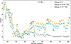 |
Fig. 1. Yield abundances from the 3 M⊙ models computed without a PMZ (grey), with ΔmPMZ = 5 × 10⁻⁴ M⊙ (cyan), and with ΔmPMZ = 10−3 M⊙ (gold). |
The light-element slide abundance pattern results from dredge-up each thermally pulsing cycle. The hydrogen shell provides the elements produced or destroyed via proton capture (e.g. Na, Mg, and Al). Additionally, this material is subject to further nucleosynthesis through neutron captures. At such low metallicities, the 22Ne source is active at this mass, with temperatures in the He shell reaching 300 MK (Table 1). The 13C neutron source is also weakly active, becoming more dominant when a 13C pocket is added. Given these available neutrons, a chain of neutron captures starting from the abundant lighter elements ensues. For example, starting from 27Al (which is produced via 26Mg(p,γ)27Al in the H-shell), the chain is essentially a light-element s-process, following closely the valley of beta stability: 27Al(n,γ)28Al(β−)28Si(n,γ)29Si(n,γ)30Si(n,γ)31Si(β−)31P, and so on. The result is the characteristic light-element abundance slide.
Hot-bottom burning also occurs at the base of the convective envelope in our model (particularly during the later thermal pulses. At around 40 MK, the HBB nucleosynthesis is not advanced, with its main effect being the conversion of dredged-up C to N via the CN cycle, giving rise to the characteristic CNO pattern dominated by N.
It can be seen that introducing a PMZ has little effect on most light elemental yields. The exceptions are P, which has an additional +1.4 dex enhancement relative to the no-PMZ model, S (+1.4 dex), Cl (+1.4 dex), and Sc (+1.8 dex). Despite these significant enhancements, we note that due to the level of dilution required to match HE 1327 (a factor of ∼1.5 dex; Sect. 3.1), enhancements over the initial composition of less than ∼1.5 dex will be of no observational consequence. This is because the ISM content will dominate for those elements. Thus, among the light elements, only C to P are expected to show significant (> 0.5 dex) enhancements in the final, diluted composition (as seen in Fig. 2).
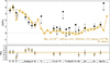 |
Fig. 2. Upper panel: Diluted yield abundances from the 3 M⊙ model with ΔmPMZ = 10−3 (gold), observed abundances (black), and upper limits (grey). Error bars are 2σ. Colour shadings represent the approximate ±0.3 dex uncertainty associated with abundances in stellar models (see the main text and Appendix A.4 for details). We show two determinations for O (solid circle from Ezzeddine et al. 2019 and open circle from Frebel et al. 2006), to highlight the uncertainty in measuring this element. Elements for which observations are unavailable are labelled in grey. Observed abundances are compiled from the literature; most are from Table 1 in Ezzeddine et al. 2019, which incorporates the 3D values from Frebel et al. 2008. Abundances for Si and Fe are from Ezzeddine & Frebel 2018. The upper limit for S is from Bonifacio et al. (2012), and V and Cr from Frebel et al. (2008). Lower panel: Residuals from the comparison. |
Phosphorus is particularly enhanced. As noted above, it is produced through a neutron capture chain starting with the lighter elements, with the final step to 31P being a β− decay after a neutron capture on 30Si (e.g. Karakas 2010). With the introduction of the PMZ and the associated increases in neutron density, this nucleosynthesis channel is enhanced. With a total enhancement of around +4 dex, this element may be observable and therefore represents a prediction of our model. We note, however, that the exact production of 31P is dependent on the uncertain rate of 30Si(n,γ) (see e.g. Fok et al. 2024).
Moving to the heavy elements, our models without a PMZ do not develop an efficient s-process. As in higher metallicity cases at this mass (e.g. Fishlock et al. 2014), 22Ne(α,n)25Mg is only marginally active as a neutron source during thermal pulses, resulting in moderate enhancements (+0.7 → +1.0 dex) of [Kr/Fe], [Rb/Fe], [Sr/Fe], [Zr/Fe], and [Ba/Fe] in the yield. The introduction of a PMZ naturally leads to considerably higher neutron densities. Successive neutron captures on 22Ne (which is refilled in every TDU episode and only partially consumed during the NeNa cycle) lead to the formation of 56Fe. This allows the s-process to continue, as described in Bisterzo et al. 2010, producing enhancements of around two orders of magnitude between Kr and Ba. These abundances rise for increasingly heavier elements up to Pb (Fig. 1). Pb itself is particularly abundant, with [Pb/Fe] reaching approximately +4 dex (around +2 dex after dilution; see the next section and Fig. 2). Pb has not yet been observed in HE 1327 and is another key prediction of our model.
Finally, our model also predicts that many elements will not be significantly enhanced: S, Cl, K, V, Cu, and Eu (see Fig. 2). This is another useful observational check for ourscenario.
3. Comparison to observations
3.1. Intermediate-mass star scenario: Our models
As described in Sect. 2.3, our scenario assumes that some chemical evolution had already occurred by [Fe/H] = −5.2, giving rise to star-forming clouds with typical enhancements of [α/Fe] = +0.5 and [Zn/Fe] = +0.7 dex (Sect. 2). From here, one of two (similar) scenarios unfolded: (i) an intermediate-mass star formed and polluted the ISM, and HE 1327 formed from that gas, or (ii) both HE 1327 and the intermediate-mass star formed at the same time in a binary system, and the intermediate-mass star enriched HE 1327 upon reaching the AGB phase. In either scenario, the chemical pattern of HE 1327 is explained by a superposition of intermediate-mass star composition onto the natal composition. As the lifetime of a 3.0 M⊙ star is 230 Myr, this sets the timescale of the scenarios. We note that the two scenarios have roughly the same timescale because it is mainly dependent on the main sequence lifetime of the star, before it reaches the AGB phase (the AGB phase is relatively short-lived). Interestingly, this is a shorter timescale than that reported from recent JWST observations, which show metals and unusually high N/O ratios very early in the Universe (440 Myr post-Big Bang; Bunker et al. 2023; Cameron et al. 2023). This lends weight to the suggestion that intermediate-mass stars significantly contributed to the ISM at that time. We note that rapidly rotating massive and very massive models could also give rise to the high N/O ratios (e.g. Nandal et al. 2024; Tsiatsiou et al. 2024).
We diluted the intermediate-mass star yields into the natal gas to mimic the ISM pollution scenario. We find that the ejecta from our intermediate-mass star must be mixed in ∼100 M⊙ of ISM matter. A dilution factor fdil = 3% of intermediate-mass star ejecta within the natal cloud provides the best overall fit to observations. Figure A.1 shows observed and theoretical abundances from some selected models. In this figure, and Fig. 2, the shaded regions around the model yield data represent an attempt to highlight their associated uncertainties. In Appendix A.4 we detail why we used 0.3 dex as an approximate abundance error. The models in Fig. A.1 generally fit within uncertainties, except for the underproduction of O. Some models overproduce Mg. Sr and Ba form with relative abundances that agree with observations ([Ba/Fe] > [Sr/Fe]), and their fit is better for increasingly larger PMZ sizes. The results from the 3.5 M⊙ model (with more efficient HBB than the lower-mass cases) with ΔmPMZ = 5 × 10⁻⁴ M⊙ are characterised by final [C/N] values lower than in the 3.0 M⊙ models, and Na, Mg and Al are overproduced. The introduction of overshooting in the 3.2 M⊙ model yields results similar to those of the 3.0 M⊙ models without overshooting.
Figure 2 shows our best fit to the observations of HE 1327: the 3.0 M⊙ model with no overshooting and ΔmPMZ = 10−3 M⊙. All abundances match within the uncertainties except for oxygen, which is 0.5 − 1.0 dex underproduced. We stress that we have not excluded any (measured) elements in our fits. The model is also consistent with all seven upper limits.
Oxygen, the one element in our model that does not fit, is challenging to measure since it suffers from substantial non-local thermodynamic equilibrium and 3D effects. In Fig. 2 we show two O abundance measurements to highlight this, from Ezzeddine et al. 2019 and Frebel et al. 20061. We note that model uncertainties may also account for this level of disagreement (0.5 − 1.0 dex in [O/Fe]). For instance, increased oxygen could come from deeper (or more numerous) TDU episodes, which depend on the poorly known convective boundaries and wind efficiency. Mixing at the bottom of the convective He flash zone can also increase surface oxygen in AGB models (Herwig 2004a) – without significantly altering the C abundance, owing to the efficiency of HBB in converting it into N.
3.2. Previous scenarios: Low-mass PIEs and supernovae
As detailed in Sect. 1, two main scenarios have so far been considered in the literature – SNe and PIEs. Here we provide quantitative comparisons between observations and models for these scenarios, using the χ2 test, as in Bisterzo et al. 2011. In this way, we aimed to see which model(s) fit best. We provide further details of these tests in Appendix A, but report the main findings here.
As discussed in the Introduction, the low-mass star PIE scenario has not met with much success in explaining HE 1327. This can be seen in panels 1 and 2 of Fig. 3, where we compare the PIE models of Campbell et al. (2010) and Cruz et al. (2013) with the observed composition of HE 1327. The 1 M⊙, [Fe/H] = −6.5 model in Campbell et al. (2010) does not reproduce the [N/Fe] > [C/Fe] > [O/Fe] pattern, overproduces the light-element slide, and severely overproduces Ba. The 1 M⊙, Z = 10−8 model of Cruz et al. (2013) could reproduce [Sr/Fe] in HE 1327, but only at the expense of overproducing C, N and O by more than two orders of magnitude. As can be seen in Fig. 3, when CNO is fit, the model fails to match Na, Mg, and Si, as well as Zn and Sr.
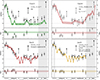 |
Fig. 3. Observed abundances of HE 1327 and observational upper limits (black) together with the yield abundances from different stellar models. Upper panels: Results from 1 M⊙ models undergoing PIEs. Lower panels: Results from massive star models undergoing SN explosions. The Z = 10−8 model (upper left) is from Cruz et al. (2013). The [Fe/H] = −5.76 (upper right) is from Campbell et al. (2010). The yields from Ezzeddine et al. (2019, lower-left panel) are from a primordial 25 M⊙ star undergoing an asymmetric mixing and fallback SN explosion. The yields from Jeena et al. (2023, lower-right panel) correspond to a rapidly rotating 12 M⊙ star of Z = 0 undergoing very efficient mixing and quasi-chemically homogeneous evolution prior to a SN explosion. The grey-shaded areas highlight the elements for which no theoretical abundances were reported. Note that in the model by Jeena et al. 2023, the authors did not consider the C and N abundances separately but instead summed them and plotted the resulting value at the location of C. We added the grey bar at the location of N to note this. As in Fig. 2, error bars are 2σ, and the shading has the same meaning. We present two determinations for O (solid circle from Ezzeddine et al. 2019 and open circle from Frebel et al. 2006) to illustrate the measurement uncertainty for this element. Observed abundances are compiled from the literature; most are from Table 1 in Ezzeddine et al. 2019, which incorporates the 3D values from Frebel et al. 2008. Abundances for Si and Fe are from Ezzeddine & Frebel 2018. The upper limit for S is from Bonifacio et al. (2012), and V and Cr from Frebel et al. (2008). Lower panel: Residuals from the comparison. The χ2 values are given in Table A.1. |
Comparisons of some representative SN model chemical patterns against observed abundances are shown in the lower panels of Fig. 3. As mentioned in the Introduction, SN models have had more success in matching the abundance pattern of HE 1327. It should be noted, however, that usually not all observed elements were part of the matches (particularly Sr) – we highlight this with grey shading in the figures.
The best fit from the aspherical bipolar jet SN model of Ezzeddine et al. 2019 (panel 3 of Fig. 3) matches all observed elements except Sr (which was not reported; Ba had not been observed yet). As mentioned in Sect. 1, Ezzeddine et al. 2019 suggested that Sr could come from fast-rotating Pop III SN progenitors. The CNO pattern, where N is highest in HE 1327, was not matched by this model – although we suggest N is within the model and observational uncertainties. Similarly to the Ezzeddine et al. 2019 model, the rapidly rotating model of Jeena et al. 2023 (Sect. 1 and panel 4 of Fig. 3) matches all of the elements except Sr (not reported). It has the same issue as the other massive star models in that the N>C>O pattern is not reproduced. In addition, Zn is only marginally reproduced.
For completeness, we briefly describe some earlier SN models for HE 1327. The model of Iwamoto et al. (2005), a 25 M⊙ faint (E < 1051erg) core-collapse SN with mixing and fallback, reproduced the Na–Mg–Al slide and the Ca abundance, but failed to explain the [N/Fe] > [C/Fe] > [O/Fe] pattern and the formation of Ni, Zn, Sr, and Ba. Takahashi et al. 2014 fitted HE 1327 with the yields from a low-energy rotating SN of 20 M⊙. This model reproduced C, O and the light-element slide but significantly underproduced N and Si. No elements heavier than Si were reported.
Finally, we considered the recent hyper-metal-poor and primordial models of Roberti et al. (2024, also see Frischknecht et al. 2012, 2016). These are fast-rotating models that include heavy elements. As noted earlier, fast-rotating models can produce the Sr and Ba. However, the yields of these models differ strongly from the observed abundance pattern of HE 1327. None of the three characteristic patterns of the star – the CNO pattern, the light-element slide, or the heavy elements – is reproduced. The main reason for this discrepancy is probably that these models do not implement the mixing–fallback mechanism to compute the explosive yields (Maeda & Nomoto 2003; Umeda & Nomoto 2003), an explosion model originally proposed to reproduce the chemical patterns of extremely metal-poor stars, and subsequently applied in various forms in the literature (for instance, in the SN models that we present in Fig. 3, and analyse in Appendix A). While primordial and hyper-metal-poor fast-rotating stars may still play a role in GCE or in shaping the abundance patterns of many CEMP stars, the current fast-rotating models considered in the context of a single-polluter scenario fail to account for the observed composition of HE 1327.
In summary, for the Pop III SN scenario, some of the fits have been reasonably successful, although they have systematically disregarded the detection of [Sr/Fe] ≈ +1 dex, and have not been able to match the CNO pattern reliably. We note in the context of these massive star/SN models that the observed [Ba/Sr] ≃ +0.2 dex suggests the operation of the main s-process (or possibly r-process) and likely rules out the weak s-process expected from massive stars.
Overall, we find that intermediate-mass models perform comparably to or even better than the best-fitting SN models, especially when all the observed species are considered (see χ2 Case A in Table A.1).
4. Summary and conclusions
Although often categorised as a CEMP-no star, we argue that, given its enhanced [N/Fe], [Sr/Fe], and (recently reported) [Ba/Fe], HE 1327 should instead be categorised as a N-CEMP-s star – and that the question of its origin should be revisited. We propose that the composition pattern of HE 1327 is a result of a superposition of a chemical yield from an intermediate-mass AGB star (∼3 M⊙) onto a primitive cloud, which had a typical composition pattern at the time. This superposition could have occurred through either binary mass transfer or the pre-pollution of HE 1327’s formation cloud by the AGB star. Interestingly, we find that the high Zn content (and α-element content) of HE 1327 can be explained by GCE – Zn is observed to increase at the lowest metallicities. We tested our scenario by comparing the observed abundances of HE 1327 to our theoretical yields of intermediate-mass stars diluted with primitive gas cloud material.
Our best-fitting model simultaneously reproduces the full range of light and heavy elements observed in HE 1327. The exception is O, which is underproduced, but we note the difficulties in determining its observed abundance and the uncertainty in stellar models. We emphasise that, unlike SN models in the literature intended to explain the composition pattern of HE 1327, our model also matches Sr and Ba and does not require exotic stellar evolution scenarios, just standard intermediate-mass star evolution.
We note, however, that HE 1327 is an atypical star at this metallicity. It stands out due to its s-process enrichment, which is not seen in other stars of comparable metallicity. Thus, our AGB plus early GCE scenario may not apply more generally at such early times.
Our models also point to a possible way to differentiate between high- and intermediate-mass star pollution – by observing P and Pb. Intermediate-mass star models with a PMZ yield significantly higher [P/Fe] and [Pb/Fe] values than standard SN models. Nevertheless, alternative models of massive stars involving rotation and nucleosynthesis in convective-reactive regions might also account for the existence of P (Masseron et al. 2020).
In conclusion, our results imply that, at metallicity [Fe/H] ∼ −5.2, the ISM already showed some degree of homogeneity and that intermediate-mass stars formed and polluted this environment; we have evidence of remnants of these pioneering stars in HE 1327. We note that models of Pop III star formation suggest that intermediate-mass stars could have formed very early on (e.g. Sharda et al. 2021) and that recent observations from JWST show metals and an unusually high N/O ratio just 440 Myr after the Big Bang (Bunker et al. 2023; Cameron et al. 2023). Although this composition has so far been attributed to rotating massive stars, this timescale is also compatible with the ∼230 Myr lifetimes of ancient stars of around 3 M⊙. These stars produce high concentrations of N as well.
The first observations of HE 1327 (Frebel et al. 2005; Aoki et al. 2006) only provided upper thresholds for [O/Fe] (< 4.0 dex). Frebel et al. (2006) revisited 1D local thermodynamic equilibrium abundances with VLT/UVES including 3D-1D corrections (Asplund 2005), and estimated a correction for 3D effects of −0.9 dex, reducing [O/Fe] from +3.7 to +2.8. Frebel et al. (2008) confirmed the 1D abundances at higher S/N and proposed a more physically sound 3D-correction technique. This resulted in a smaller 3D correction leading to [O/Fe] = +3.4 dex. The later [Fe/H] correction in Ezzeddine & Frebel (2018) led to the currently recommended [O/Fe] = +3.14 dex.
Acknowledgments
This work was supported by the Spanish projects PID2019-109363GB-100, PID2023-148661NB-I00, by the AGAUR/Generalitat de Catalunya grant SGR-386/2021, and by the Deutsche Forschungsgemeinschaft, DFG project number Ts 17/2–1. SWC acknowledges federal funding from the Australian Research Council through a Future Fellowship (FT160100046) and Discovery Projects (DP190102431 & DP210101299). ML acknowledges funding from the LP2023-10 Lendulet grant of the Hungarian Academy of Sciences. Parts of this research was supported by the Australian Research Council Centre of Excellence for All Sky Astrophysics in 3 Dimensions (ASTRO 3D), through project number CE170100013. This research was supported by use of the Nectar Research Cloud, a collaborative Australian research platform supported by the National Collaborative Research Infrastructure Strategy (NCRIS).
References
- Abia, C., & Rebolo, R. 1989, ApJ, 347, 186 [Google Scholar]
- Aoki, W., Frebel, A., Christlieb, N., et al. 2006, ApJ, 639, 897 [Google Scholar]
- Asplund, M. 2005, ARA&A, 43, 481 [Google Scholar]
- Beers, T. C., & Christlieb, N. 2005, ARA&A, 43, 531 [NASA ADS] [CrossRef] [Google Scholar]
- Beyer, W. H. 1991, CRC Standard Mathematical Tables and Formulae (CRC Press) [Google Scholar]
- Bisterzo, S., Gallino, R., Straniero, O., Cristallo, S., & Käppeler, F. 2010, MNRAS, 404, 1529 [NASA ADS] [Google Scholar]
- Bisterzo, S., Gallino, R., Straniero, O., Cristallo, S., & Käppeler, F. 2011, MNRAS, 418, 284 [Google Scholar]
- Bloecker, T. 1995, A&A, 297, 727 [Google Scholar]
- Böhm-Vitense, E. 1958, Z. Astrophys., 46, 108 [Google Scholar]
- Bonifacio, P., Caffau, E., Venn, K. A., & Lambert, D. L. 2012, A&A, 544, A102 [NASA ADS] [CrossRef] [EDP Sciences] [Google Scholar]
- Bunker, A. J., Saxena, A., Cameron, A. J., et al. 2023, A&A, 677, A88 [NASA ADS] [CrossRef] [EDP Sciences] [Google Scholar]
- Buntain, J. F., Doherty, C. L., Lugaro, M., et al. 2017, MNRAS, 471, 824 [NASA ADS] [CrossRef] [Google Scholar]
- Cameron, A. J., Katz, H., Rey, M. P., & Saxena, A. 2023, MNRAS, 523, 3516 [NASA ADS] [CrossRef] [Google Scholar]
- Campbell, S. W. 2008, Ph.D. Thesis, Monash University, Australia, [arXiv:2410.21972] [Google Scholar]
- Campbell, S. W., & Lattanzio, J. C. 2008, A&A, 490, 769 [NASA ADS] [CrossRef] [EDP Sciences] [Google Scholar]
- Campbell, S. W., Lugaro, M., & Karakas, A. I. 2010, A&A, 522, L6 [NASA ADS] [CrossRef] [EDP Sciences] [Google Scholar]
- Cannon, R. C. 1993, MNRAS, 263, 817 [NASA ADS] [CrossRef] [Google Scholar]
- Choplin, A., Hirschi, R., Meynet, G., & Ekström, S. 2017, A&A, 607, L3 [NASA ADS] [CrossRef] [EDP Sciences] [Google Scholar]
- Collet, R., Asplund, M., & Trampedach, R. 2006, ApJ, 644, L121 [NASA ADS] [CrossRef] [Google Scholar]
- Constantino, T., Campbell, S., Gil-Pons, P., & Lattanzio, J. 2014, ApJ, 784, 56 [NASA ADS] [CrossRef] [Google Scholar]
- Constantino, T., Campbell, S. W., Christensen-Dalsgaard, J., Lattanzio, J. C., & Stello, D. 2015, MNRAS, 452, 123 [Google Scholar]
- Cruz, M. A., Serenelli, A., & Weiss, A. 2013, A&A, 559, A4 [NASA ADS] [CrossRef] [EDP Sciences] [Google Scholar]
- Cyburt, R. H., Amthor, A. M., Ferguson, R., et al. 2010, ApJS, 189, 240 [NASA ADS] [CrossRef] [Google Scholar]
- Dillmann, I., Heil, M., Käppeler, F., et al. 2006, in Capture Gamma-Ray Spectroscopy and Related Topics, eds. A. Woehr, & A. Aprahamian, AIP Conf. Ser., 819, 123 [NASA ADS] [CrossRef] [Google Scholar]
- Doherty, C. L., Siess, L., Lattanzio, J. C., & Gil-Pons, P. 2010, MNRAS, 401, 1453 [NASA ADS] [CrossRef] [Google Scholar]
- Ezzeddine, R., & Frebel, A. 2018, ApJ, 863, 168 [Google Scholar]
- Ezzeddine, R., Frebel, A., Roederer, I. U., et al. 2019, ApJ, 876, 97 [NASA ADS] [CrossRef] [Google Scholar]
- Fishlock, C. K., Karakas, A. I., Lugaro, M., & Yong, D. 2014, ApJ, 797, 44 [Google Scholar]
- Fok, H. K., Pignatari, M., Côté, B., & Trappitsch, R. 2024, ApJ, 977, L24 [Google Scholar]
- Frebel, A., Aoki, W., Christlieb, N., et al. 2005, Nature, 434, 871 [CrossRef] [Google Scholar]
- Frebel, A., Christlieb, N., Norris, J. E., Aoki, W., & Asplund, M. 2006, ApJ, 638, L17 [Google Scholar]
- Frebel, A., Collet, R., Eriksson, K., Christlieb, N., & Aoki, W. 2008, ApJ, 684, 588 [NASA ADS] [CrossRef] [Google Scholar]
- Frischknecht, U., Hirschi, R., & Thielemann, F.-K. 2012, A&A, 538, L2 [NASA ADS] [CrossRef] [EDP Sciences] [Google Scholar]
- Frischknecht, U., Hirschi, R., Pignatari, M., et al. 2016, MNRAS, 456, 1803 [Google Scholar]
- Frost, C. A., & Lattanzio, J. C. 1996, ApJ, 473, 383 [NASA ADS] [CrossRef] [Google Scholar]
- Gaia Collaboration (Brown, A. G. A., et al.) 2018, A&A, 616, A1 [NASA ADS] [CrossRef] [EDP Sciences] [Google Scholar]
- Gil-Pons, P., Doherty, C. L., Gutiérrez, J. L., et al. 2018, PASA, 35 [Google Scholar]
- Gil-Pons, P., Doherty, C. L., Gutiérrez, J., et al. 2021, A&A, 645, A10 [EDP Sciences] [Google Scholar]
- Gil-Pons, P., Doherty, C. L., Campbell, S. W., & Gutiérrez, J. 2022, A&A, 668, A100 [NASA ADS] [CrossRef] [EDP Sciences] [Google Scholar]
- Grevesse, N., Noels, A., & Sauval, A. J. 1996, in Cosmic Abundances, eds. S. S. Holt, & G. Sonneborn, ASP Conf. Ser., 99, 117 [Google Scholar]
- Hansen, T. T., Andersen, J., Nordström, B., et al. 2016, A&A, 588, A3 [NASA ADS] [CrossRef] [EDP Sciences] [Google Scholar]
- Heil, M., Detwiler, R., Azuma, R. E., et al. 2008, Phys. Rev. C, 78, 025803 [CrossRef] [Google Scholar]
- Herwig, F. 2004a, ApJ, 605, 425 [NASA ADS] [CrossRef] [Google Scholar]
- Herwig, F. 2004b, ApJS, 155, 651 [Google Scholar]
- Herwig, F., Bloecker, T., Schoenberner, D., & El Eid, M. 1997, A&A, 324, L81 [NASA ADS] [Google Scholar]
- Iliadis, C., Longland, R., Champagne, A. E., Coc, A., & Fitzgerald, R. 2010, Nucl. Phys. A, 841, 31 [CrossRef] [Google Scholar]
- Ishigaki, M. N., Tominaga, N., Kobayashi, C., & Nomoto, K. 2014, ApJ, 792, L32 [NASA ADS] [CrossRef] [Google Scholar]
- Iwamoto, N., Umeda, H., Tominaga, N., Nomoto, K., & Maeda, K. 2005, Science, 309, 451 [NASA ADS] [CrossRef] [Google Scholar]
- Izzard, R. G., Glebbeek, E., Stancliffe, R. J., & Pols, O. R. 2009, A&A, 508, 1359 [NASA ADS] [CrossRef] [EDP Sciences] [Google Scholar]
- Jeena, S. K., Banerjee, P., Chiaki, G., & Heger, A. 2023, MNRAS, 526, 4467 [Google Scholar]
- Karakas, A. I. 2010, MNRAS, 403, 1413 [NASA ADS] [CrossRef] [Google Scholar]
- Karakas, A., & Lattanzio, J. C. 2007, PASA, 24, 103 [NASA ADS] [CrossRef] [Google Scholar]
- Karakas, A. I., & Lattanzio, J. C. 2014, PASA, 31, e030 [NASA ADS] [CrossRef] [Google Scholar]
- Kobayashi, C., Karakas, A. I., & Lugaro, M. 2020, ApJ, 900, 179 [Google Scholar]
- Korn, A. J., Richard, O., Mashonkina, L., et al. 2009, ApJ, 698, 410 [Google Scholar]
- Lattanzio, J. C. 1986, ApJ, 311, 708 [NASA ADS] [CrossRef] [Google Scholar]
- Lattanzio, J., Frost, C., Cannon, R., & Wood, P. R. 1996, Mem. Soc. Astron. It., 67, 729 [Google Scholar]
- Lederer, M. T., & Aringer, B. 2009, A&A, 494, 403 [NASA ADS] [CrossRef] [EDP Sciences] [Google Scholar]
- Lucatello, S., Tsangarides, S., Beers, T. C., et al. 2005, ApJ, 625, 825 [NASA ADS] [CrossRef] [Google Scholar]
- Lugaro, M., Karakas, A. I., Stancliffe, R. J., & Rijs, C. 2012, ApJ, 747, 2 [Google Scholar]
- Maeda, K., & Nomoto, K. 2003, ApJ, 598, 1163 [NASA ADS] [CrossRef] [Google Scholar]
- Maeder, A., & Meynet, G. 2015, A&A, 580, A32 [NASA ADS] [CrossRef] [EDP Sciences] [Google Scholar]
- Marigo, P., & Aringer, B. 2009, A&A, 508, 1539 [CrossRef] [EDP Sciences] [Google Scholar]
- Mashonkina, L., Sitnova, T., & Belyaev, A. K. 2017, A&A, 605, A53 [NASA ADS] [CrossRef] [EDP Sciences] [Google Scholar]
- Masseron, T., García-Hernández, D. A., Santoveña, R., et al. 2020, Nat. Commun., 11, 3759 [NASA ADS] [CrossRef] [Google Scholar]
- Meynet, G., Ekström, S., & Maeder, A. 2006, A&A, 447, 623 [NASA ADS] [CrossRef] [EDP Sciences] [Google Scholar]
- Molaro, P., Aguado, D. S., Caffau, E., et al. 2023, A&A, 679, A72 [NASA ADS] [CrossRef] [EDP Sciences] [Google Scholar]
- Nandal, D., Sibony, Y., & Tsiatsiou, S. 2024, A&A, 688, A142 [NASA ADS] [CrossRef] [EDP Sciences] [Google Scholar]
- Pols, O. R., Izzard, R. G., Stancliffe, R. J., & Glebbeek, E. 2012, A&A, 547, A76 [NASA ADS] [CrossRef] [EDP Sciences] [Google Scholar]
- Ritter, J. S., Safranek-Shrader, C., Gnat, O., Milosavljević, M., & Bromm, V. 2012, ApJ, 761, 56 [Google Scholar]
- Ritter, C., Herwig, F., Jones, S., et al. 2018, MNRAS, 480, 538 [NASA ADS] [CrossRef] [Google Scholar]
- Roberti, L., Limongi, M., & Chieffi, A. 2024, ApJS, 270, 28 [NASA ADS] [CrossRef] [Google Scholar]
- Saito, Y.-J., Takada-Hidai, M., Honda, S., & Takeda, Y. 2009, PASJ, 61, 549 [NASA ADS] [Google Scholar]
- Sharda, P., Federrath, C., Krumholz, M. R., & Schleicher, D. R. G. 2021, MNRAS, 503, 2014 [NASA ADS] [CrossRef] [Google Scholar]
- Straniero, O., Gallino, R., Busso, M., et al. 1995, ApJ, 440, L85 [NASA ADS] [CrossRef] [Google Scholar]
- Straniero, O., Cristallo, S., & Piersanti, L. 2014, ApJ, 785, 77 [NASA ADS] [CrossRef] [Google Scholar]
- Takahashi, K., Umeda, H., & Yoshida, T. 2014, ApJ, 794, 40 [Google Scholar]
- Tominaga, N., Umeda, H., & Nomoto, K. 2007, ApJ, 660, 516 [NASA ADS] [CrossRef] [Google Scholar]
- Tominaga, N., Iwamoto, N., & Nomoto, K. 2014, ApJ, 785, 98 [NASA ADS] [CrossRef] [Google Scholar]
- Tsiatsiou, S., Sibony, Y., Nandal, D., et al. 2024, A&A, 687, A307 [NASA ADS] [CrossRef] [EDP Sciences] [Google Scholar]
- Umeda, H., & Nomoto, K. 2002, ApJ, 565, 385 [Google Scholar]
- Umeda, H., & Nomoto, K. 2003, Nature, 422, 871 [NASA ADS] [CrossRef] [PubMed] [Google Scholar]
- Ventura, P., D’Antona, F., Mazzitelli, I., & Gratton, R. 2001, ApJ, 550, L65 [CrossRef] [Google Scholar]
- Yong, D., Norris, J. E., Bessell, M. S., et al. 2013, ApJ, 762, 27 [Google Scholar]
- Yoon, J., Beers, T. C., Placco, V. M., et al. 2016, ApJ, 833, 20 [Google Scholar]
Appendix A: Details of comparisons between models and observations
A.1. Dilution
According to our proposed scenario, the ejecta from our intermediate-mass stars are mixed with the natal cloud material.
We defined the dilution factor (fdil) as
 (A.1)
(A.1)
where Mej is the mass ejected by one of our model stars, and Mcl is the mass of the natal cloud. Taking Mi, ej and Mi, cl, respectively, as the ejected and cloud masses of species ‘i’, the mass fraction of each species is
 (A.2)
(A.2)
Thus, Xi, ⋆ can be expressed in terms of the ejecta abundances Xi, ej and cloud abundances Xi, cl:
 (A.3)
(A.3)
After converting from mass to number abundances (Yi, ej and Yi, cl) our theoretical abundance of each species, in the standard notation, is then given by
![Mathematical equation: $$ \begin{aligned} \mathrm {[X_i/Fe]}=\log _{10}\left(\frac{Y_i}{\mathrm{{Y_{Fe}}}} \right)_\star - \log _{10}\left(\frac{Y_i}{Y_{Fe}} \right)_\odot . \end{aligned} $$](/articles/aa/full_html/2025/11/aa56363-25/aa56363-25-eq6.gif) (A.4)
(A.4)
The resulting theoretical abundances for selected elements, initial masses (Mini), and PMZ masses (ΔmPMZ) are shown in Table B.1.
A.2. Abundance pattern comparisons: χN2 test
We calculated χN2 as in Bisterzo et al. 2011, to assess and compare the quality of our fits with those existing in the literature,
![Mathematical equation: $$ \begin{aligned} \chi _N^2=\sum _{i=1}^N \frac{\Bigl (\mathrm {[X_i/Fe]} - \mathrm {[X_i/Fe]_{obs}}\Bigr )^2}{\epsilon _i^2} ,\end{aligned} $$](/articles/aa/full_html/2025/11/aa56363-25/aa56363-25-eq7.gif) (A.5)
(A.5)
where [Xi/Fe] have been described above, [Xi/Fe]obs are the analogous observed abundances, ϵ is the observational error corresponding to 2σ, and N is the number of considered elements in the observed data (with error bars).
Table A.1 summarises our results for the χ2 test for different cases. Case A considers all elements detected (i.e. excluding those with upper limits). Case B considers the same species as Case A but excludes the single element that provides the worst fit between theoretical and observed abundances. This case allows us to disregard the effects of possible outliers, which are interpreted as those species whose abundances may be particularly problematic to determine observationally or are especially sensitive to theoretical input physics and uncertainties. Case C further relaxes the statistical comparison, excluding the two worst-fitting elements. Moreover, this case allows us to consider the comparison between the observed data and the SN models by Ezzeddine et al. 2019 and Jeena et al. 2023, who did not account for the presence of Sr and Ba in their fits.
The results of the χ2 test, shown in Table A.1, imply the following:
-
i)
When all the elements are considered (Case A), we obtain the best probability distribution (or confidence level) value for the intermediate-mass models. Our best-fitting model (3 M⊙ with a mPMZ = 10−3 M⊙) yields Pn(χ2) = 52%, whereas the SN models from Ezzeddine et al. 2019 and Jeena et al. 2023, unable to produce heavy elements, yield Pn(χ2) below 10%.
-
ii)
When we discard the single worst-fitting element (Case B), the Pn(χ2) value for our 3 M⊙ with a mPMZ = 10−3 M⊙ increases up to 81%. Oxygen is the element that most significantly affects the quality of the fits of all the 3 M⊙ models. As reported in Sect. 3.1, oxygen is a difficult species to measure in the case of HE 1327. On the other hand, our models naturally suffer from input physics uncertainties that affect theoretical abundances. Increasing the overall efficiency of TDU (through diffusive overshooting at the base of the pulse-driven convective zone (Herwig 2004a) or a larger number of TDU episodes than computed here, possibly due to less efficient stellar winds) would result in higher theoretical oxygen abundances, accompanied by slightly higher heavy-element abundances. Both trends would improve the fit to observed values even more.
-
iii)
The fit of SN models when disregarding Ba increases to Pn(χ2) = 28% and 51% for the models by Ezzeddine et al. 2019 and Jeena et al. 2023, respectively.
-
iv)
Case C (when we disregard the two worst-fitting species) recovers very high confidence levels for the SN models. However, our best-fitting model performs considerably better than the SN fit in Ezzeddine et al. 2019 (Pn(χ2) = 94% versus 86%), and very close to the fit in Jeena et al. 2023, with Pn(χ2) = 97%.
To further assess our comparison analysis, we calculated modified versions of the χ2 test. First, we considered including species for which observations have determined the upper limits. If theoretical abundances remained below these limits (as was the case for all the considered models), no term was added to calculate the χ2 value, but the number of degrees of freedom increased to account for species with upper limits. Consequently, the confidence levels improved considerably. For Case A, the best-fitting intermediate-mass model yielded Pn(χ2) = 87%, and the best SN fit (Jeena et al. 2023) yielded Pn(χ2) = 35%. For Case B, Pn(χ2) = 98% for the best-fitting intermediate-mass model and 76% for the SN model, respectively. Finally, all models yielded Pn(χ2)≥97% for Case C.
Results for the χN2 performed for different models.
A.3. Summary of χ2 comparisons
In conclusion, we find that the intermediate-mass models fit the observed abundances of HE 1327 considerably better than the SN models when all the observed species (or all except the worst-fitting species) are considered. This holds irrespective of whether we consider elements for which only upper limits were determined. When we exclude the two worst-fitting elements, the best-fitting SN model performs just slightly better than the best-fitting intermediate-mass model.
We present the abundance patterns visually, comparing them to observations for our models in Fig. A.1. For the newest SN and low-mass models from the literature, we provide a comparison in Fig. 3.
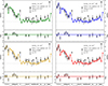 |
Fig. A.1. Theoretical yield abundances (post-dilution) together with the observed abundances of HE 1327, as in Fig. 2. See Table B.1 for numerical values. Model parameters are given in each panel (see also Sect. 2 and Table 1). The residuals and shaded areas have the same meaning as in Fig. 2. The χ2 values are given in Table A.1. |
A.4. Model yield uncertainties
In Figures 2, 3 and A.1 we attempt to highlight the uncertainties in model yields by including some shading around our values. These uncertainties primarily arise from our limited understanding of internal mixing processes, the location of convective boundaries, mass-loss rates, and, in some cases, nuclear reaction rates. Quantifying these uncertainties is complicated, so we opted to consider the range of yield variations from models by different authors in the existing literature. For instance, Ritter et al. (2018) compared results from Karakas (2010) and Straniero et al. (2014) of 2 M⊙ models of Z = 10−4. The yield differences in dex are ΔKS(C) = |Log(YK10(C)−Log(YS14(C))| = 0.36. Analogously, for N and O, ΔKS(N) = 0.26 and ΔKS(O) = 0.30. Comparisons between the yields from Ritter et al. (2018) and Karakas (2010) yielded similar values (somewhat lower for C), or considerably higher (ΔKR(O)≃1). Comparing published yields for 3 M⊙ of Z = 10−4 models yields ΔKS(C) = 0.30, ΔKS(N) = 0.13 and ΔKS(O) = 0.07, and ΔKR(C) = 0.42, ΔKR(N) = 0.41 and ΔKR(O) = 0.72. Considering that uncertainties increase even more for lower-metallicity models, we took a Δ of ±0.3 dex as a conservative value for our analysis. As a reference, Gil-Pons et al. (2021) analysed the effects of different standard wind prescriptions on stellar yields and found variations that, in all cases, were higher than 0.4 dex. For more on model uncertainties, we refer the interested reader to Karakas & Lattanzio (2014) for a general overview and to Gil-Pons et al. (2018) for the specific case of extremely low-metallicity stars.
Appendix B: Model abundances
In Table B.1 we list the elemental yields for our grid of models, after dilution with the primitive cloud composition (see Sect. 2).
Final composition (in [X/H]) of our models after dilution.
All Tables
All Figures
|
Fig. 1. Yield abundances from the 3 M⊙ models computed without a PMZ (grey), with ΔmPMZ = 5 × 10⁻⁴ M⊙ (cyan), and with ΔmPMZ = 10−3 M⊙ (gold). |
| In the text | |
|
Fig. 2. Upper panel: Diluted yield abundances from the 3 M⊙ model with ΔmPMZ = 10−3 (gold), observed abundances (black), and upper limits (grey). Error bars are 2σ. Colour shadings represent the approximate ±0.3 dex uncertainty associated with abundances in stellar models (see the main text and Appendix A.4 for details). We show two determinations for O (solid circle from Ezzeddine et al. 2019 and open circle from Frebel et al. 2006), to highlight the uncertainty in measuring this element. Elements for which observations are unavailable are labelled in grey. Observed abundances are compiled from the literature; most are from Table 1 in Ezzeddine et al. 2019, which incorporates the 3D values from Frebel et al. 2008. Abundances for Si and Fe are from Ezzeddine & Frebel 2018. The upper limit for S is from Bonifacio et al. (2012), and V and Cr from Frebel et al. (2008). Lower panel: Residuals from the comparison. |
| In the text | |
|
Fig. 3. Observed abundances of HE 1327 and observational upper limits (black) together with the yield abundances from different stellar models. Upper panels: Results from 1 M⊙ models undergoing PIEs. Lower panels: Results from massive star models undergoing SN explosions. The Z = 10−8 model (upper left) is from Cruz et al. (2013). The [Fe/H] = −5.76 (upper right) is from Campbell et al. (2010). The yields from Ezzeddine et al. (2019, lower-left panel) are from a primordial 25 M⊙ star undergoing an asymmetric mixing and fallback SN explosion. The yields from Jeena et al. (2023, lower-right panel) correspond to a rapidly rotating 12 M⊙ star of Z = 0 undergoing very efficient mixing and quasi-chemically homogeneous evolution prior to a SN explosion. The grey-shaded areas highlight the elements for which no theoretical abundances were reported. Note that in the model by Jeena et al. 2023, the authors did not consider the C and N abundances separately but instead summed them and plotted the resulting value at the location of C. We added the grey bar at the location of N to note this. As in Fig. 2, error bars are 2σ, and the shading has the same meaning. We present two determinations for O (solid circle from Ezzeddine et al. 2019 and open circle from Frebel et al. 2006) to illustrate the measurement uncertainty for this element. Observed abundances are compiled from the literature; most are from Table 1 in Ezzeddine et al. 2019, which incorporates the 3D values from Frebel et al. 2008. Abundances for Si and Fe are from Ezzeddine & Frebel 2018. The upper limit for S is from Bonifacio et al. (2012), and V and Cr from Frebel et al. (2008). Lower panel: Residuals from the comparison. The χ2 values are given in Table A.1. |
| In the text | |
|
Fig. A.1. Theoretical yield abundances (post-dilution) together with the observed abundances of HE 1327, as in Fig. 2. See Table B.1 for numerical values. Model parameters are given in each panel (see also Sect. 2 and Table 1). The residuals and shaded areas have the same meaning as in Fig. 2. The χ2 values are given in Table A.1. |
| In the text | |
Current usage metrics show cumulative count of Article Views (full-text article views including HTML views, PDF and ePub downloads, according to the available data) and Abstracts Views on Vision4Press platform.
Data correspond to usage on the plateform after 2015. The current usage metrics is available 48-96 hours after online publication and is updated daily on week days.
Initial download of the metrics may take a while.