| Issue |
A&A
Volume 703, November 2025
|
|
|---|---|---|
| Article Number | A91 | |
| Number of page(s) | 5 | |
| Section | The Sun and the Heliosphere | |
| DOI | https://doi.org/10.1051/0004-6361/202556528 | |
| Published online | 07 November 2025 | |
Heavy ion differential streaming observed in small-scale flux ropes
Institute for Experimental and Applied Physics (IEAP), Christian Albrechts University at Kiel, Leibnizstr. 11, 24118 Kiel, Germany
⋆ Corresponding author: This email address is being protected from spambots. You need JavaScript enabled to view it.
Received:
21
July
2025
Accepted:
16
September
2025
Abstract
Context. In the collisionless solar wind, different ion species propagate with different speeds. The respective nonzero differential streaming of an ion species (i) with speed vi relative to the proton speed (vp), i.e., vi − p = vi − vp, is associated with wave activity in a nonthermal plasma. Yet wave activity is expected to be weak in flux ropes where the magnetic field exhibits a smooth rotation.
Aims. We evaluated wave activity within small-scale flux ropes (SFRs) with different scale sizes and background solar wind conditions, with differential streaming as a reliable tracer, at a 12-minute time resolution.
Methods. Based on measurements from the Advanced Composition Explorer (ACE), we reconstructed the differential velocity between He2+ and protons (vHe2+−p) in over 18 000 SFRs detected at 1 au. We then conducted a statistical study to check the overall status of differential streaming therein.
Results. The differential streaming is weak in SFRs inside interplanetary coronal mass ejections (ICMEs) and magnetic clouds (MCs) detected by ACE at 1 au. Regarding SFRs outside ICMEs and MCs, about 40% exhibit rather strong differential streaming, i.e., streaming exceeds 0.6 times the local Alfvén speed. Such SFRs also tend to have collisionally young and fast plasma.
Conclusions. Our results suggest that the identification of wave activity might be underestimated by the criteria used to construct the available SFR list. Differential streaming appears to be a more reliable tracer of wave activity.
Key words: Sun: coronal mass ejections (CMEs) / Sun: magnetic fields / solar wind
© The Authors 2025
 Open Access article, published by EDP Sciences, under the terms of the Creative Commons Attribution License (https://creativecommons.org/licenses/by/4.0), which permits unrestricted use, distribution, and reproduction in any medium, provided the original work is properly cited.
This article is published in open access under the Subscribe to Open model. This email address is being protected from spambots. You need JavaScript enabled to view it. to support open access publication.
1. Introduction
Differential streaming between helium and protons is often seen in high-speed collisionally young solar wind (Asbridge et al. 1976; Ran et al. 2024; Mostafavi et al. 2024) and is also reported in switchbacks (Huang et al. 2023) and stream interaction regions (Ďurovcová et al. 2019). It is likewise well-documented for other heavier ions streaming relative to protons in the solar wind (Ogilvie et al. 1982; Schmidt et al. 1980; von Steiger et al. 1995; Berger et al. 2011; Gu et al. 2024). The phenomenon is not fully understood, though the wave–particle interaction, which may further cause preferential heating and acceleration (Ofman 2004), is one promising interpretation (Gary et al. 2000a,b). The maintenance of differential streaming is also thought to be regulated by hydromagnetic waves (Marsch et al. 1982; Marsch & Livi 1987). The differential streaming is considered to be aligned with the magnetic field and is efficiently decreased by Coulomb collisions (Kasper et al. 2008). At 1 au, the ion–proton differential velocity stays comparable to, but generally lower than, the local Alfvén speed (VA). The differential flow speeds of most ion species lie within 0.55 ± 0.15VA (Berger et al. 2011) at 1 au, and the differential velocity decreases with distance from the Sun and with proton speed (Neugebauer et al. 1996).
Flux ropes (FRs), which figuratively describe twisted magnetic configurations that coil around a central axis (Russell & Elphic 1979), can be observed as a coherent rotation of the magnetic field in the in situ measurements made by spacecrafts. Magnetic clouds (MCs) were the earliest discovered FRs and are the most commonly identified FRs; their diameters at 1 au fall in the range 0.2–0.4 au (Lepping et al. 1990). Small-scale flux ropes (SFRs) are FRs that are as much as ten times smaller than typical MCs. SFRs have been widely identified through in situ measurements via different methods (Moldwin et al. 2000; Feng et al. 2007).
The differences between MCs and SFRs (except regarding their sizes) are still a matter of debate. Cartwright & Moldwin (2008, 2010) suggested that the distribution of FRs exhibits a double peak, with MCs and SFRs showing distinct characteristics in in-situ data, such as proton temperatures and expansion rates. Janvier et al. (2014) suggested that SFRs are not associated with coronal mass ejections (CMEs), and that only MCs can serve as counterparts to CMEs because SFRs are so numerous.
Zhang et al. (2024) conclude that the ion–proton differential streaming is generally negligible in interplanetary coronal mass ejections (ICMEs), which contain a lot of MCs. This is expected since a typical feature of ICMEs and MCs is that they have low magnetic fluctuation. It is unknown whether there is any ion–proton differential streaming in SFRs, and it is worthwhile to compare SFRs inside and outside ICMEs, and include MCs as a reference.
We compared the derived measurements of differential streaming of He2+ and protons with respect to SFRs with different scale sizes and background solar wind conditions. The data used in this work and the lists from which the SFRs, ICMEs, and MCs were taken are presented in Sect. 2, as is a related data analysis method. Results are presented in Sect. 3, which is followed by discussions and conclusions in Sect. 4.
2. Data, event lists, and methods
This work used multiple data products from different instruments on board the Advanced Composition Explorer (ACE; Stone et al. 1998). The heavy ion data are in 12-minute time resolution, measured by the Solar Wind Ion Composition Spectrometer (SWICS; Gloeckler et al. 1998) from 2001 to 2010. The SWICS comprises a time-of-flight mass spectrometer and an electrostatic analyzer. It measures the mass, charge, and energy of solar wind particles. A subset of the data is available as high-resolution pulse-height-analyzed data; a detailed and extensive description of the data analysis procedure applied to the pulse-height-analyzed data is given in Berger’s PhD thesis (Berger 2008). SWICS in principle can only measure |vi|, but vi − p is assumed to be parallel to the magnetic field. With the knowledge of vp and B, the |vi − p|=|vi − vp| can be calculated (Berger et al. 2011), where vi and vp are the vector velocities.
Magnetic field data come from the Magnetometer (MAG; Smith et al. 1998) at 16-second time resolution. Solar wind proton plasma data come from the Solar Wind Electron Proton Alpha Monitor (SWEPAM; McComas et al. 1998) at 64-second time resolution. These data are provided by the ACE Science Center1. Based on the magnetic field data and proton plasma data, three parameters were further calculated and synchronized with SWICS data. The proton-proton collisional age (Acol; Kasper et al. 2008) in this work is defined as
 (1)
(1)
where np is the proton number density, vp is the proton speed, and Tp is the proton temperature. The Alfvénicity parameter (CvB; Roberts et al. 1987; Bavassano et al. 1998) is defined as
 (2)
(2)
where δ denotes the fluctuation from the mean value. The local Alfvén speed (VA) is defined as
 (3)
(3)
where B is the magnetic field strength, ρ is the mass density of the plasma, and μ0 is the permeability of free space.
The ICMEs used in this study were compiled from two sources: the list by Cane & Richardson (2003) and Richardson & Cane (2010), and the list by Jian et al. (2011, 2006). Both lists are available from the ACE Science Center2. The ICME start time is defined as the shock arrival time, when available. An SFR was considered associated with an ICME if it shares at least one data point with the ICME. An SFR was considered “outside ICMEs” if its nearest ICME is more than 6 hours away. The MC list comes from Marubashi & Lepping (2007), provided by the Korea Astronomy and Space Science Institute3.
This study mainly used the FR list4 based on the Grad-Shafranov reconstruction technique (Hu et al. 2018; Hu & Sonnerup 2002). A detailed description of the technique as well as the detailed technical procedures with control flow and data flow can be found in Hu (2017). This list was chosen because the identification method has been applied to the same spacecraft that measures the heavy ions, i.e., ACE, it has been widely applied in other related studies (Huang et al. 2020; Xu et al. 2020; Zhai et al. 2023), and it includes more smaller FRs compared to other lists.
In the selected SFR list, the upper and lower limits of FR duration were manually set to 2165 minutes and 9 minutes for ACE data. In practice, the detection was split into multiple iterations separated by different-width search windows applied to the time-series data with one-minute cadence, from 9–16 minutes to 2159–2166 minutes. Each iteration identifies FR candidates whose duration fell within the specified time range. Thus, in the SFR list, the time resolution of FR boundaries is 1 minute.
For many SFRs, the timescale of their encounters with spacecraft is comparable to the time resolution of SWICS. Consequently, it was critical to determine whether a specific 12-minute interval that is partly covered by an SFR should be considered within or outside the event. Zhai et al. (2023) adopted the 2-hour resolution data at the starting or ending part of a FR if more than half of the time interval represented by this data point is occupied by the FR. However, this is not physically well motivated.
In each 12-minute measurement interval, the SWICS electrostatic analyzer is stepped through 60 logarithmical steps from 100 kV down to 0.49 kV. As a result, each 12-minute measurement interval can be further divided into 60 equal-length sub-intervals. The energy-per-charge step recorded by SWICS then represents a specific sub-interval, and the related time stamp of this sub-interval can be obtained. The particle counts that were detected during each energy-per-charge step (sub-interval) are recorded as well; thus, within each 12-min interval, the ratio between counts that were completely within the SFR period and the overall number of counts can be obtained. If this ratio is larger than a high threshold, then the majority of particles detected during this 12-minute interval belong to this SFR. This threshold was set to 95% in this study. All 12-minute measurement intervals that are partially covered by SFR periods were evaluated independently. As a result, some SFRs, even those shorter than 12 minutes, could be taken into account, which increased the total sample size. Of the 5867 SFRs shorter than 12 minutes on the SFR list, 1520 were assigned a valid SWICS measurement interval according to this boundary policy. For higher-resolution MAG data and SWEPAM data, the boundary policy was defined based on a direct comparison between the time stamps of spacecraft measurements and the boundaries of SFRs.
3. Results
This section presents the main results related to He2+-proton differential streaming found in SFRs. They are linked to the scale size and duration in Fig. 1, and to other kinetic properties and locations relative to other structures in Fig. 2.
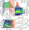 |
Fig. 1. (a) Distribution of average |vHe2+ − p|/VA (bin size = 0.02). The blue (pink) area indicates weak (strong) differential streaming. (b) Scale size distributions of SFRs with strong or weak differential streaming (logarithmic bins, |


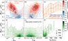 |
Fig. 2. (a) Contour plots of the joint distributions between the average |vHe2+ − p|/VA and collisional age (Acol). SFRs within (outside) ICMEs are plotted in blue (red), and counts are normalized to the overall maximum. Bin sizes are |

Overall, there are 25701 SFRs on the SFR list, among which 18135 have sufficient data to calculate the average |vHe2+ − p|/VA, which characterizes the intensity of differential streaming. A clear peak appears around |vHe2+ − p|/VA = 0.7 in Fig. 1a, and another around |vHe2+ − p|/VA = 0.2, which indicates contributions of cases with weak differential streaming. In this study, we defined d|vHe2+ − p|/VA ≥ 0.6 as “strong” differential streaming and |vHe2+ − p|/VA ≤ 0.2 as “weak” differential streaming. There are 6650 SFRs with average |vHe2+ − p|/VA ≥ 0.6 (strong SFRs) and 3339 SFRs with average |vHe2+ − p|/VA ≤ 0.2 (weak SFRs).
Figure 1b shows the scale size distributions of strong SFRs (pink) and weak SFRs (blue). They both peak around 4 × 10⁻³ au, which is the typical scale size of SFRs, and the number of strong SFRs is about three time that of weak SFRs at the peak value. The distribution of weak SFRs has a heavier tail at larger scale sizes compared to strong SFRs. That heavy tail extends to 10−1 au, which is close to the typical scale size of MCs.
In panel c, SFRs are classified by their durations, which correspond to the number of SWICS data points (Nmeas) they cover (one data point represents one 12-minute time interval). Measurement intervals partially covered by SFRs are treated based on the boundary policy presented in Sect. 2. The kernel density estimation functions are shown here normalized to their own maximum. In this work, 64% SFRs are short (Nmeas ≤ 2, blue and orange curves), while they are the main contributors of the right peak in panel a. For slightly longer SFRs (17.4%, green and red curves), the heights of the left and right peaks are roughly equal. For SFRs longer than 4 hours (3%, dashed line), the left peak is clear, while the right peak almost vanishes. Combining SFRs in between (solid black line), the dominant peak transitions from right to left as the duration increases. Panels b and c together show that small or short SFRs more frequently have a higher average |vHe2+ − p|/VA, while VA does not show a clear scale size dependence in panel d.
The low average |vHe2+ − p|/VA frequently found in longer SFRs could result from an averaging effect. The definition of strong or weak SFRs based on this average value can thus also be problematic. We further investigated the averaging effect by breaking SFRs longer than 1 hour (Nmeas ≥ 5) down into every data point. Panel e shows the distribution of related standard deviations (σ|vHe2+ − p|/VA). SFRs with strong and weak differential streaming generally have smaller σ|vHe2+ − p|/VA compared to SFRs, with an intermediate |vHe2+ − p|/VA value. Panels f and g together examine our definition of “strong” and “weak” by showing how many individual strong (Ns with |vHe2+ − p|/VA ≥ 0.6) and weak data points (Nw with |vHe2+ − p|/VA ≤ 0.2) are contained in strong and weak SFRs, respectively. The result is straightforward: in general, 80% of the data points of weak SFRs are themselves weak (see blue points in panel g). Strong SFRs have similar results, though the proportion of strong points decreases with fluctuations when Ns≥18. Panels e to g show that the average |vHe2+ − p|/VA is representative and the definition of strong and weak based on that average value isreliable.
The results shown in Fig. 1 indicate that strong differential streaming is more frequently observed in SFRs with scale sizes below 10−2 au, while weak or no differential streaming is seen in SFRs with scale sizes of up to 10−1 au. Furthermore, such strong or weak differential streaming observed in SFRs tends to be a “global” feature; most data points are strong (weak) within strong (weak) cases. The definition of strong and weak SFRs and their average |vHe2+ − p|/VA are thus reliable.
Figure 2 compares |vHe2+ − p|/VA with other solar wind properties. In panels a and b, parameters are averaged for each case, and SFRs are further divided into the 15266 cases outside ICMEs and the 2216 cases in ICMEs (the 653 cases close to an ICME are omitted). All data points covered by MCs and time periods that are neither SFRs nor ICMEs are plotted in the other four panels as references. The contour plots in panels a and b clearly show that SFRs outside ICMEs (red) often exhibit strong differential streaming, while SFRs in ICMEs (blue) are more MC-like (green, panels d and e), where weak or no differential streaming is expected in general.
In detail, panel a shows that high |vHe2+ − p|/VA is more often related to SFRs outside ICMEs with low Acol. At the same Acol level, the |vHe2+ − p|/VA usually is higher in SFRs outside ICMEs compared to those inside ICMEs or MC plasma (panel d), and the difference becomes smaller when Acol increases. The anticorrelation between |vHe2+ − p|/VA and Acol is expected because differential steaming is stronger in fast (and collisionally young) solar wind. This anticorrelation is evident in panel c, where the proton velocity is plotted along the x-axis: the relationship between differential streaming and solar wind speed in non-SFR, non-ICME solar wind is consistent with that for SFRs outsideICMEs.
As previously stated, differential streaming is an indicator of wave activity. In panel b, CvB is plotted as a second proxy for wave activity. Though the most frequent CvB in SFRs outside ICMEs is around 0.7, which is larger than that of SFRs in ICMEs and that of MCs (panel e), the correlations between |vHe2+ − p|/VA and CvB are unclear considering the large error bars. Some SFRs, whether inside or outside ICMEs, exhibit large CvB but not necessarily high |vHe2+ − p|/VA. In such cases, wave activity may still be present but not captured by differential streaming. The differences between SFRs inside and outside ICMEs are more pronounced for |vHe2+ − p|/VA thanfor CvB.
The results shown in Fig. 2 illustrate that SFRs outside ICMEs are different from those inside ICMEs with respect to differential streaming. Strong differential streaming is more often seen in SFRs outside ICMEs, especially when those SFRs have small Acol and large CvB. There is no evidence that the differential streaming observed in SFRs is distinct from that in non-SFR, non-ICME solar wind. SFRs in ICMEs, however, areMC-like.
4. Discussion and conclusions
We verified that the differential streaming is generally weak in SFRs inside ICMEs, similar to differential streaming in MCs. However, rather strong ion-proton differential streaming, represented by |vHe2+ − p|/VA ≥ 0.6, is observed in about 40% of SFRs (outside ICMEs) detected by ACE at 1 au. The observed strong (or weak) differential streaming likely extends throughout the entire SFR. The plasma within SFRs with strong differential streaming also tends to be collisionally young, fast, and Alfvénic (typical of coronal-hole wind properties). We also verified that results related to O6+, C5+, and Fe9 + ,10 + ,11+ are similar, but they are not presented here.
The ion–proton differential streaming within SFRs is generally consistent with that of the surrounding solar wind. However, it is difficult to properly define the “background” solar wind for individual SFRs due to limited temporal distances (in the measurements) between two neighboring SFRs. Only about 9% of the SFRs in this work have at least one hour of solar wind measurements before and after them without the involvement of any other FRs (Gu 2025).
Strong ion-proton differential streaming indicates non-thermalized plasma, which further hints at the existence of strong wave activity. This is unexpected in an ideal FR, where the magnetic field should exhibit a smooth rotation with only minimal fluctuations. That is the case for MCs (see Fig. 2), which are considered easier to identify. Relatively large SFRs also rarely exhibit strong differential streaming (see Figs. 1b and 1c). The SFRs analyzed here are taken from a list that defines them as “static FRs” with low Alfvénicity (Chen et al. 2021), yet strong ion–proton differential streaming is observed. Potential wave activity may have led to false identifications of some SFRs, especially at their typical scale size (∼4 × 10⁻³ au). Neither the CvB in this work nor the proton field-aligned flow in Chen et al. (2021) can perfectly represent the Alfvénicity in SFRs, though ion–proton differential streaming may be able to.
In addition, ion-proton differential streaming can transport heavy-ion signatures between the surrounding plasma and structures defined independently of ion measurements (such as SFRs), a factor that should be considered when studying heavy-ion composition, particularly in small structures. In situ measurements of heavy ions closer to Solar Orbiter (Müller et al. 2020; Owen et al. 2020), when they are fully calibrated, are expected to reveal more details of ion–proton differential streaming because of the higher time resolution and higher heavy ion density.
http://www.srl.caltech.edu/ACE/ASC/level2 (Retrieved August, 1, 2023).
http://www.srl.caltech.edu/ACE/ASC/DATA/level3/index.html (Retrieved April 21, 2022).
https://sos.kasi.re.kr/mc/ (Retrieved August, 19, 2024).
http://fluxrope.info/ (Retrieved Jan, 12, 2024).
Acknowledgments
Chaoran Gu is supported by German Space Agency (DLR) grant number WI 2139/12-1. Verena Heidrich-Meisner is supported by German Space Agency (DLR) grant number 50OC2104.
References
- Asbridge, J. R., Bame, S. J., Feldman, W. C., & Montgomery, M. D. 1976, J. Geophys. Res., 81, 2719 [NASA ADS] [CrossRef] [Google Scholar]
- Bavassano, B., Pietropaolo, E., & Bruno, R. 1998, J. Geophys. Res., 103, 6521 [NASA ADS] [CrossRef] [Google Scholar]
- Berger, L. 2008, Ph.D. Thesis, Kiel University, Germany [Google Scholar]
- Berger, L., Wimmer-Schweingruber, R. F., & Gloeckler, G. 2011, Phys. Rev. Lett., 106, 151103 [NASA ADS] [CrossRef] [Google Scholar]
- Cane, H. V., & Richardson, I. G. 2003, J. Geophys. Res. (Space Phys.), 108, 1156 [NASA ADS] [CrossRef] [Google Scholar]
- Cartwright, M. L., & Moldwin, M. B. 2008, J. Geophys. Res. (Space Phys.), 113, A09105 [Google Scholar]
- Cartwright, M. L., & Moldwin, M. B. 2010, J. Geophys. Res. (Space Phys.), 115, A08102 [NASA ADS] [Google Scholar]
- Chen, Y., Hu, Q., Zhao, L., Kasper, J. C., & Huang, J. 2021, ApJ, 914, 108 [NASA ADS] [CrossRef] [Google Scholar]
- Ďurovcová, T., Němeček, Z., & Šafránková, J. 2019, ApJ, 873, 24 [CrossRef] [Google Scholar]
- Feng, H. Q., Wu, D. J., & Chao, J. K. 2007, J. Geophys. Res. (Space Phys.), 112, A02102 [Google Scholar]
- Gary, S. P., Yin, L., & Winske, D. 2000a, Geophys. Res. Lett., 27, 2457 [Google Scholar]
- Gary, S. P., Yin, L., Winske, D., & Reisenfeld, D. B. 2000b, Geophys. Res. Lett., 27, 1355 [Google Scholar]
- Gloeckler, G., Cain, J., Ipavich, F. M., et al. 1998, Space Sci. Rev., 86, 497 [NASA ADS] [CrossRef] [Google Scholar]
- Gu, C. 2025, Ph.D. Thesis, Kiel, Germany [Google Scholar]
- Gu, C., Heidrich-Meisner, V., & Wimmer-Schweingruber, R. F. 2024, A&A, 692, A191 [NASA ADS] [CrossRef] [EDP Sciences] [Google Scholar]
- Hu, S. Q. 2017, Sci. China Earth Sci., 60, 1466 [Google Scholar]
- Hu, Q., & Sonnerup, B. U. Ö. 2002, J. Geophys. Res. (Space Phys.), 107, 1142 [Google Scholar]
- Hu, Q., Zheng, J., Chen, Y., le Roux, J., & Zhao, L. 2018, ApJS, 239, 12 [Google Scholar]
- Huang, J., Liu, Y., Liu, J., & Shen, Y. 2020, ApJ, 899, L29 [Google Scholar]
- Huang, J., Kasper, J. C., Fisk, L. A., et al. 2023, ApJ, 952, 33 [NASA ADS] [CrossRef] [Google Scholar]
- Janvier, M., Démoulin, P., & Dasso, S. 2014, Sol. Phys., 289, 2633 [Google Scholar]
- Jian, L., Russell, C. T., Luhmann, J. G., & Skoug, R. M. 2006, Sol. Phys., 239, 393 [NASA ADS] [CrossRef] [Google Scholar]
- Jian, L. K., Russell, C. T., & Luhmann, J. G. 2011, Sol. Phys., 274, 321 [Google Scholar]
- Kasper, J. C., Lazarus, A. J., & Gary, S. P. 2008, Phys. Rev. Lett., 101, 261103 [Google Scholar]
- Lepping, R. P., Jones, J. A., & Burlaga, L. F. 1990, J. Geophys. Res., 95, 11957 [Google Scholar]
- Marsch, E., & Livi, S. 1987, J. Geophys. Res., 92, 7263 [Google Scholar]
- Marsch, E., Rosenbauer, H., Schwenn, R., Muehlhaeuser, K. H., & Neubauer, F. M. 1982, J. Geophys. Res., 87, 35 [Google Scholar]
- Marubashi, K., & Lepping, R. P. 2007, Ann. Geophys., 25, 2453 [Google Scholar]
- McComas, D. J., Bame, S. J., Barker, P., et al. 1998, Space Sci. Rev., 86, 563 [CrossRef] [Google Scholar]
- Moldwin, M. B., Ford, S., Lepping, R., Slavin, J., & Szabo, A. 2000, Geophys. Res. Lett., 27, 57 [NASA ADS] [CrossRef] [Google Scholar]
- Mostafavi, P., Allen, R. C., Jagarlamudi, V. K., et al. 2024, A&A, 682, A152 [NASA ADS] [CrossRef] [EDP Sciences] [Google Scholar]
- Müller, D., St. Cyr, O. C., Zouganelis, I., et al. 2020, A&A, 642, A1 [Google Scholar]
- Neugebauer, M., Goldstein, B. E., Smith, E. J., & Feldman, W. C. 1996, J. Geophys. Res., 101, 17047 [NASA ADS] [CrossRef] [Google Scholar]
- Ofman, L. 2004, J. Geophys. Res. (Space Phys.), 109, A07102 [Google Scholar]
- Ogilvie, K. W., Coplan, M. A., & Zwickl, R. D. 1982, J. Geophys. Res., 87, 7363 [NASA ADS] [CrossRef] [Google Scholar]
- Owen, C. J., Bruno, R., Livi, S., et al. 2020, A&A, 642, A16 [EDP Sciences] [Google Scholar]
- Ran, H., Liu, Y. D., Chen, C., & Mostafavi, P. 2024, ApJ, 963, 82 [Google Scholar]
- Richardson, I. G., & Cane, H. V. 2010, Sol. Phys., 264, 189 [NASA ADS] [CrossRef] [Google Scholar]
- Roberts, D. A., Klein, L. W., Goldstein, M. L., & Matthaeus, W. H. 1987, J. Geophys. Res., 92, 11021 [Google Scholar]
- Russell, C. T., & Elphic, R. C. 1979, Nature, 279, 616 [NASA ADS] [CrossRef] [Google Scholar]
- Schmidt, W. K. H., Rosenbauer, H., Shelly, E. G., & Geiss, J. 1980, Geophys. Res. Lett., 7, 697 [NASA ADS] [CrossRef] [Google Scholar]
- Smith, C. W., L’Heureux, J., Ness, N. F., et al. 1998, Space Sci. Rev., 86, 613 [Google Scholar]
- Stone, E. C., Frandsen, A. M., Mewaldt, R. A., et al. 1998, Space Sci. Rev., 86, 1 [Google Scholar]
- von Steiger, R., Geiss, J., Gloeckler, G., & Galvin, A. B. 1995, Space Sci. Rev., 72, 71 [NASA ADS] [CrossRef] [Google Scholar]
- Xu, M., Shen, C., Hu, Q., Wang, Y., & Chi, Y. 2020, ApJ, 904, 122 [Google Scholar]
- Zhai, C., Fu, H., Si, J., Huang, Z., & Xia, L. 2023, ApJ, 950, 79 [Google Scholar]
- Zhang, X., Song, H., Zhang, C., et al. 2024, ApJ, 967, 118 [NASA ADS] [CrossRef] [Google Scholar]
All Figures
|
Fig. 1. (a) Distribution of average |vHe2+ − p|/VA (bin size = 0.02). The blue (pink) area indicates weak (strong) differential streaming. (b) Scale size distributions of SFRs with strong or weak differential streaming (logarithmic bins, |
| In the text | |
|
Fig. 2. (a) Contour plots of the joint distributions between the average |vHe2+ − p|/VA and collisional age (Acol). SFRs within (outside) ICMEs are plotted in blue (red), and counts are normalized to the overall maximum. Bin sizes are |
| In the text | |
Current usage metrics show cumulative count of Article Views (full-text article views including HTML views, PDF and ePub downloads, according to the available data) and Abstracts Views on Vision4Press platform.
Data correspond to usage on the plateform after 2015. The current usage metrics is available 48-96 hours after online publication and is updated daily on week days.
Initial download of the metrics may take a while.