| Issue |
A&A
Volume 703, November 2025
|
|
|---|---|---|
| Article Number | A221 | |
| Number of page(s) | 12 | |
| Section | Planets, planetary systems, and small bodies | |
| DOI | https://doi.org/10.1051/0004-6361/202556560 | |
| Published online | 20 November 2025 | |
Evidence of a gap in the envelope mass fraction of sub-Saturns
1
University Observatory Munich, Faculty of Physics, Ludwig-Maximilians-Universität München,
Scheinerstr. 1,
81679
Munich,
Germany
2
Max-Planck Institute for Extraterrestrial Physics,
Giessenbachstrasse 1,
85748
Garching,
Germany
3
Max Planck Institut für Astronomie,
Königstuhl 17,
69117
Heidelberg,
Germany
★ Corresponding author: This email address is being protected from spambots. You need JavaScript enabled to view it.
Received:
23
July
2025
Accepted:
17
September
2025
Abstract
Under the core-accretion model, gas giants form via runaway accretion. This process starts when the mass of the accreted envelope becomes equal to the mass of the core. We modeled a population of warm sub-Saturns to search for imprints of their formation history in their internal structure. Using the GAS gianT modeL for Interiors (GASTLI), we calculated a grid of interior structure models on which we performed retrievals for our sample of 28 sub-Saturns to derive their envelope mass fractions (fenv). For each planet, we ran three different retrievals, assuming low (−2.0<log (Fe/H)<0.5), medium (0.5<log (Fe/H)<1.4), and high (1.4<log (Fe/H)<1.7) atmospheric metallicity. The distribution of fenv in our sample was then compared to outcomes and predictions of planet formation models. When our results are compared to the outcomes of a planetesimal accretion formation model, we find that we require a high atmospheric metallicity for intermediate-mass sub-Saturns to reproduce the simulated planet population. For higher planetary masses, a medium atmospheric metallicity provides the best agreement. Additionally, we find a bimodal distribution of fenv in our sample with a gap that is located at different values of fenv for different atmospheric metallicities. For the high atmospheric metallicity case, the gap in the fenv distribution is located between 0.5 and 0.7, which is consistent with assumptions of the core-accretion model in which runaway accretion starts when Menv ≈ Mcore(fenv is ∼ 0.5). We also find a bimodal distribution of the hydrogen and helium mass fraction (fH/He) with a gap at fH/He=0.3. The location of this gap is independent of the assumed atmospheric metallicity. Lastly, we compared the distributions of our sub-Saturns in the Neptunian savanna to a population of sub-Saturns in the Neptune desert and ridge. We find that the observed fenv distribution of savanna and ridge sub-Saturns is consistent with the planets coming from the same underlying population.
Key words: planets and satellites: composition / planets and satellites: gaseous planets / planetary systems
© The Authors 2025
 Open Access article, published by EDP Sciences, under the terms of the Creative Commons Attribution License (https://creativecommons.org/licenses/by/4.0), which permits unrestricted use, distribution, and reproduction in any medium, provided the original work is properly cited.
This article is published in open access under the Subscribe to Open model.
Open Access funding provided by Max Planck Society.
1 Introduction
The prevailing theory to explain the formation of gas-rich planets is the core-accretion model (Mizuno et al. 1978; Mizuno 1980; Stevenson 1982; Bodenheimer & Pollack 1986; Lissauer 1993; Pollack et al. 1996). In this paradigm, solid cores with several times the Earth’s mass (∼ 10−20 M⊕) accrete gas from the surrounding protoplanetary disk. Initially, the accretion rate is set by the atmosphere’s cooling time (Lee & Chiang 2015; Ginzburg et al. 2016). After the mass of the gaseous envelope reaches the mass of the core, the self-gravity of the atmosphere is no longer negligible and the planet enters a stage of runaway accretion, when it is able to accrete gas at a much faster rate (Perri & Cameron 1974; Mizuno 1980; Stevenson 1982; Pollack et al. 1996; Lee et al. 2014).
Under this assumption of core accretion, gaseous planets can be divided into two groups. The first comprises planets that never reached an envelope mass fraction (fenv=Menv /(Menv+Mcore)) of 50% and thus do not start runaway accretion. These planets would likely have an internal structure similar to that of Neptune and Uranus (fenv ∼ 10−25%, Miguel & Vazan 2023). The second is gas giants that started runaway accretion and acquired a massive envelope (fenv of ∼ 80−100%), with internal structures similar to those of Jupiter and Saturn (Miguel & Vazan 2023). Planets with fenv of ∼ 50−70% should be rare as they would have started the process of runaway accretion but then somehow quickly stopped accreting, leading to only a moderate gain in envelope mass (Ida & Lin 2004; Mordasini et al. 2009). While these planets could have started runaway accretion just shortly before the protoplanetary disk dispersed, the required coincidence of these two rapid processes makes it unlikely.
As the population of known exoplanets grows, we can look for imprints of the core-accretion model on the population of gaseous planets. Intermediate-sized exoplanets (4 R⊕<Rp< 8 R⊕), often called super-Neptunes or sub-Saturns (hereinafter sub-Saturns; Hartman et al. 2009; Petigura et al. 2017), are key targets to study, as we expect the transition to runaway gas accretion to happen in this regime. Short-period sub-Saturns are well studied, with a known paucity of sub-Saturns on very short orbits, called the Neptune desert (Lecavelier Des Etangs 2007; Szabó & Kiss 2011; Beaugé & Nesvorný 2013; Sanchis-Ojeda et al. 2014; Lundkvist et al. 2016; Mazeh et al. 2016). The responsible mechanism for this desert is more likely connected to the long-term evolution of these planets due to the proximity to their stellar hosts, rather than their formation. The most favored explanations include a combination of atmospheric escape (Kurokawa & Nakamoto 2014; Jackson et al. 2017; Owen 2019; Koskinen et al. 2022) and migration mechanisms (Matsakos & Königl 2016; Owen & Lai 2018; Vissapragada et al. 2022).
Recently, Bourrier et al. (2023) reported an underdensity of sub-Saturns even with longer orbital periods, which they named the Neptunian savanna. The Neptunian savanna is separated from the Neptune desert by an overdensity of sub-Saturns with periods between 3.2 and 5.7 days, coined the Neptunian ridge (Castro-González et al. 2024a), which coincides with the hot-Jupiter pileup (Udry et al. 2003). Given that planets in the savanna are influenced less strongly by their host stars, it could be a remnant of formation through core accretion and runaway accretion. However, as a large portion of these planets are expected to form beyond the ice line and then migrate inward, it is unclear how well the observed population represents their primordial distribution. If runaway accretion is indeed responsible for the deficit of sub-Saturns with longer periods, this should be reflected in the distribution of fenv.
The envelope mass fraction can be estimated from the observed planetary masses and radii through models of their interior structure. A two-component model composed of an Earth-composition core and a H/He envelope (Lopez & Fortney 2014) has been used to derive individual envelope mass fractions of sub-Saturns (Petigura et al. 2016, 2017; Thomas et al. 2025). These models found fenv to be ≥ 50% for some of these planets, which should be unlikely according to core-accretion and runaway gas accretion theories (Petigura et al. 2018, 2020; Mistry et al. 2023). Millholland et al. (2020) show that for close-in sub-Saturns, tidal heating can inflate the radii of these planets, causing these simple models to overestimate fenv by up to 60%. After considering tidal inflation, most close-in sub-Saturns in their sample had fenv similar to that of Neptune. Although the exact reduction in envelope fraction depends on a couple of unknowns, such as the tidal quality factor and the obliquity (Millholland et al. 2020).
Another limitation of previous studies that used internal structure models to estimate fenv is the assumption of a pure H/He envelope, which is inconsistent with the Solar System gas planets and their varying levels of envelope enrichment (Irwin et al. 2014; Guillot & Gautier 2015). Additionally, some sub-Saturns have been shown to have high-metallicity atmospheres (MacDonald & Madhusudhan 2019), and both interior structure modeling (Thorngren et al. 2016) and planet formation models (Cridland et al. 2020; Danti et al. 2023) suggest that planets in this mass range should be metal-rich. During envelope accretion, solid objects in the form of pebbles and/or planetesimals are accreted along with the gas. If the gaseous envelope is sufficiently dense to evaporate these bodies before they reach the core, the atmosphere will be polluted with metals (Pollack et al. 1986; Alibert 2017; Lozovsky et al. 2017; Brouwers et al. 2018). Envelope enrichment significantly influences the formation of giant planets by reducing the critical core mass for runaway accretion and thus shortening the timescales for giant planet formation (Ikoma et al. 2000; Hori & Ikoma 2011; Venturini et al. 2016; Valletta & Helled 2020). On the other hand, Alibert et al. (2018) suggest that an intermediate stage of efficient heavy element accretion will delay the onset of runaway accretion until Mp reaches ∼ 100 M⊕. This could explain the observed differences in bulk metallicity between Saturn and Jupiter since Saturn would not have started runaway accretion in this case (Venturini & Helled 2020; Helled 2023).
In this work, we analyzed the population of warm sub-Saturns to connect their observed properties to planet formation theory. We used the GAS gianT modeL for Interiors (GASTLI; Acuña et al. 2024, 2021) interior structure modeling code1 to derive envelope mass fractions for our sample. GASTLI expands the simple two-component model by taking the atmospheric metallicity into account for a more accurate calculation of the planet’s interior structure. Using GASTLI, we calculated a grid of interior-structure models on which we performed interior structure retrievals on our sample of sub-Saturns to analyze the distribution of fenv. In Sect. 2, we present the selection of our sub-Saturn sample and how we recomputed the ages for all the stars in this sample. Section 3 describes the computation of the interior structure model grid on which the retrievals were performed. The results are presented in Sect. 4. In Sect. 5, we compare our results to the planet formation model of Alessi et al. (2020) and discuss the observed distribution of fenv in the context of core accretion.
2 Sample selection
2.1 Planet selection
The planets in our sample were selected according to the following criteria to enable modeling with GASTLI and minimize the effects of interaction between the star and planet. We used the NASA Exoplanet Archive (Christiansen et al. 2025) composite table of confirmed planets.
The planets need to have measured radii and masses for the retrieval. We limited our sample to planets in the radius range between 4 and 10 R⊕. Typically, sub-Saturns are defined between 4 and 8 R⊕. We extended this radius range to include a few planets in the Jovian planet population that are certain to have undergone runaway accretion to compare with the sub-Saturns. The lower limit on the mass of our targets (Mp>15 M⊕) is driven by GASTLI’s default atmospheric grid (see Acuña et al. 2024, for details). We did not impose an upper mass limit; however, all the planets in the final sample have masses of ≤ 1 MJ. The planetary radius is much more sensitive to the envelope mass fraction than to the mass. As such, we required a radius measurement precision of σR<20%. In order not to bias the sample too much, and in an effort to maintain meaningful number statistics, we did not impose strict requirements on the mass precision and included all planets with a true mass measurement (i.e., no upper limits).
Orbital periods longer than 15 days. Millholland et al. (2020) show that the tidal forces that close-in planets are subjected to can cause radius inflation, which in turn leads to an overestimation of fenv. This effect is strongest in planets with P<10 days and additionally depends on the eccentricity and obliquity of the planet. To limit the influence of tidal inflation on our derivation of fenv, we imposed an orbital period limit on the sample. The only planet in our sample with an eccentricity larger than 0.5 is TOI-2134
 . However, given the large period of 95 days, we do not expect tidal inflation to be strong enough to significantly affect the derived fenv.
Planet equilibrium temperature <1000 K. The atmospheric grid we used for GASTLI is only valid up to equilibrium temperatures of 1000 K. The equilibrium temperatures were calculated following Eq. (23) in Acuña et al. (2024), assuming a global average (fav=4).
2.2 Age determination
A key parameter to perform interior structure retrievals from observed radii and masses is the age of the planet. Planets contract over their lifetime as they cool after their formation. The change in radius is strongest in the first 1−2 Gyr, which makes it difficult to infer the interior structure from observed properties for young planets. To derive accurate envelope mass fractions for young planets, the age should ideally be known with a precision of 10% (Müller & Helled 2023). For planets older than 2 Gyr, the precision requirement can be relaxed. We calculated the ages for all planets in the sample using the Python code stardate (Angus et al. 2019), which combines isochrone fitting with gyrochronology to infer precise stellar ages. We used the stellar effective temperature (Teff), the metallicity (Fe/H), and broadband photometry from Gaia (G, GRP, and GBP) and 2MASS (J, H, and K) as input for the isochrone fitting. For the gyrochronology, we estimated the rotation period (Prot) of the star from spectroscopic v sin (i) measurements and the stellar radii. Since the measured v sin (i) is only a lower limit for the rotational velocity of the star, the calculated Prot only gives an upper limit. For some planets, Prot could be determined from brightness modulations in their light curves. We ensured that our calculated Prot matches the photometric values in these cases. The calculated ages for all stars are listed in Table A.1. We also list the literature ages of the stars where available.
To ensure that we could derive accurate fenv, we limited the sub-Saturn sample to planets that are older than 1 Gyr within 1 σ. The average uncertainty of the ages derived in this work (1.1 Gyr) is smaller than that of the literature ages (1.9 Gyr). From the 28 stars in our sample that had literature ages, only 6 did not agree within their 1 σ uncertainties, and only K2-24 does not agree within 2 σ. Given the large error on the rotational period, it is possible that stardate might overestimate the age of the star compared to a calculation method that does not include gyrochronology. However, since both the literature and the stardate age are well above 1 Gyr, this discrepancy should not affect the derived fenv. Of the stars that made it into the sample, only Kepler-9 would have been excluded based on the literature age. On the other Hand, there are six stars that were excluded based on their re-derived ages, even though the literature ages were within our requirements. This means that there is likely no contamination from young stars in our sample, which could skew the results. However, it is possible that some of the excluded planets could in fact be older and therefore should have been included in the sample.
In total, we were left with 28 sub-Saturns in our sample. They are all listed in Table B.1. The majority of planets have orbital periods of <50 days due to the increasingly low transit probability at larger separations. Figure 1 shows a mass-radius diagram of the planets in our sample in the context of the larger exoplanet population. The radii of the planets in our sample are evenly distributed over the whole range of sub-Saturn radii with a small gap between 6 and 7 R⊕. There are three high-density planets in our sample that are isolated compared to the rest of the population.
3 Interior structure retrieval
3.1 Interior-atmosphere model grid
Using GASTLI, we first calculated a grid of interior structure models on which to perform retrievals to derive envelope mass fractions for our sub-Saturn sample. GASTLI solves the differential equations of planetary interior structure on a onedimensional grid, assuming conservation of mass, hydrostatic equilibrium, convection, and thermal evolution due to secular cooling. It uses state-of-the-art equations of state for H/He, water, and rock (see the references in Acuña et al. 2024) to compute density and entropy. GASTLI assumes two compositional layers: a metal-rich core and an envelope. The core composition is fixed to a 1: 1 mass ratio of water and rock (see also Thorngren et al. 2016), while the envelope consists of H/He with water as a proxy for metals. The mass fraction of metals in the envelope, Zenv, is defined as a user input parameter.
The interior structure model is coupled to a grid of atmospheric models via an iterative algorithm (Acuña et al. 2021). This approach allows the temperature at the interior-atmosphere boundary to be calculated self-consistently. We also used the atmospheric pressure-temperature profile to integrate the equation of hydrostatic equilibrium and compute the atmospheric thickness, which contributes to the total planetary radius. For this calculation, we assumed a transit pressure of 20 mbar, which corresponds to the pressure level probed by transit photometry (Grimm et al. 2018). Further details of the implementation are given in Acuña et al. (2024, 2025). GASTLI uses a default atmospheric grid generated with petitCODE. PetitCODE solves the radiative transfer equation and applies the Schwarzschild criterion to obtain self-consistent atmospheric pressure-temperature profiles and Bond albedos. More details on petitCODE, including its atmospheric species and the references of their opacity tables, can be found in Mollière et al. (2015, 2017).
The interior-atmosphere models in GASTLI take the following inputs: planetary mass (Mp), internal temperature (Tint), equilibrium temperature (Teq), core mass fraction (CMF=1− fenv), and atmospheric metallicity (log (Fe/H)). The equilibrium temperature is calculated as a global average and assuming a null Bond albedo, consistent with the input of the petitCODE grid (see Eq. (23) in Acuña et al. 2024). The effective temperature of the atmosphere is given by  , where Tint is an input, and the Bond albedo (AB) is computed selfconsistently by petitCODE. The planet’s internal heat is
  , where σSB is the Stefan-Boltzmann constant. Given these five input parameters – Mp, Tint, Teq, CMF and log (Fe/H) – the model output parameters are the total radius (Rtot), the age, the total metal mass fraction (Zplanet=CMF+fenv × Zenv), and the atmospheric metal mass fraction (Zenv). Zenv is equivalent to log (Fe/H) but expressed as a mass fraction instead of solar units.
The input masses in our grid range between 0.05 MJ and 1.05 MJ. For the lower masses, the grid has a finer spacing of 0.01 MJ as the absolute errors in the planet masses are smaller. Between 0.2 MJ and 0.5 MJ grid points are 0.03 MJ apart. From 0.5 MJ until 1.05 MJ we used a spacing of 0.05 MJ. The equilibrium temperature grid spans values from 300 to 1000 K in steps of 50 K. For the atmospheric metallicity, we used values of – 2.0, 0.0, 1.0, and 1.7 dex. We calculated the internal structure at internal temperatures of 50 K, 100 K, 200 K, 300 K, and 400 K.
The lower limits of planetary mass and atmospheric metallicity are set by GASTLI’s atmospheric grid. Since our sample consists only of mature planets, the internal temperature range covered by the grid is sufficient to encompass their ages. The equilibrium temperatures in our sample range from 295 K to 999 K. The upper limit on atmospheric metallicity, set at 50 × solar, is motivated by two factors. First, this value corresponds to the highest envelope metallicity observed in Neptunemass exoplanets (Wakeford et al. 2018), while Neptune has an atmospheric metallicity of 80 × solar. Thus, more massive exoplanets in our sample are expected to have metallicities lower than 50−80 × solar. Second, GASTLI’s default atmospheric grid extends the interior-atmosphere interface pressure (Psurf) to 1000 bar for log (Fe/H)<2. At higher metallicities, Psurf must be reduced to ∼ 10 bar. This pressure range ensures convergence of the petitCODE atmospheric models. Moreover, at these pressures, the atmosphere is convective due to the high opacity, such that the adiabatic (convective) temperature profile computed by GASTLI avoids spurious temperature jumps at the interior-atmosphere boundary.
This change in surface pressure can produce irregular entropy-age and radius-age curves, which require validation. Therefore, we adopted the 50 × solar metallicity limit and validated the thermal evolution curves on a case-by-case basis. This involved identifying models in which the surface pressure changes. For those cases, we either adopted the values from the last stable point for the subsequent time steps or interpolated between two valid models. This approximation does not affect the forward models, as these occur at low internal temperatures, where the planetary radius remains constant with age (see Fig. 2).
The validation of our GASTLI grid involves ensuring all models are in hydrostatic equilibrium. Some of the models in our grid with the lowest CMFs and planet masses are not in hydrostatic equilibrium due to the low surface gravity. For these models, GASTLI does not converge because they are unphysical. We consequently replaced these points with NaNs in our grid. This affected roughly 3% of the models. In total, our grid consists of 42180 models. We have made the grid publicly available via Zenodo (https://zenodo.org/records/17396266).
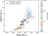 |
Fig. 1 Mass-radius diagram of the sub-Saturns in our sample. The colored points show the exoplanet population with radii and masses measured to the precision of our selection criteria. Their colors indicate the orbital periods of the planets. The sub-Saturns that were analyzed in this work are overplotted in black. |
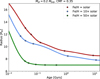 |
Fig. 2 Thermal evolution curves for a planet with a CMF of 0.35 and a mass of 0.2 MJ with varying atmospheric metallicities. The input internal temperatures are converted to ages, and the planet radius at each step is calculated by GASTLI. A higher assumed atmospheric metallicity leads to a lower total radius. After ∼ 1 Gyr, the change in radius due to the contraction of the planetary envelope is small even for low-metallicity atmospheres. |
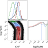 |
Fig. 3 Corner plots of the interior structure retrieval for Kepler-280b. Shown in black is the retrieval without any constraint on log (Fe/H). While the CMF is uncorrelated for the majority of log (Fe/H) values, for high atmospheric metallicities the inferred CMF decreases significantly. To illustrate this, the contours for low (−2.0<log (Fe/H)<0.5), medium (0.5<log (Fe/H)≤1.4), and high (1.4<log (Fe/H)<1.7) atmospheric metallicity retrievals are overplotted in red, blue, and green, respectively. |
3.2 Retrieval setup
Following the approach in Acuña et al. (2024), we applied a Markov chain Monte Carlo framework to retrieve posterior distributions for the interior structure parameters of the planets in our sample, using emcee (Foreman-Mackey et al. 2013). The log-likelihood was calculated using the radii, masses, and ages of our planets (see Eqs. (6) and (14) in Dorn et al. 2015; Acuña et al. 2021):
 (1)
We found that there were only marginal differences in the results when fitting for the equilibrium temperature compared to running the retrieval with Teq fixed to the closest node in our grid. To reduce computational time, we therefore fixed Teq in the following analysis. The rest of the parameters are given uniform priors spanning the full range of our grid. We used 32 walkers with 200,000 steps while checking convergence using the autocorrelation time, τ (ensuring ≪ N/50).
(1)
We found that there were only marginal differences in the results when fitting for the equilibrium temperature compared to running the retrieval with Teq fixed to the closest node in our grid. To reduce computational time, we therefore fixed Teq in the following analysis. The rest of the parameters are given uniform priors spanning the full range of our grid. We used 32 walkers with 200,000 steps while checking convergence using the autocorrelation time, τ (ensuring ≪ N/50).
When running the retrievals on the full range of log (Fe/H) values, we found that there is a strong degeneracy between the inferred envelope mass fraction and the atmospheric metallicity (see Fig.3). For small atmospheric metallicities (log (Fe/H)<0.5), fenv does not vary significantly with the atmospheric metallicity. However, for a high value of log (Fe/H), the inferred fenv can differ from the low-metallicity scenario by up to 0.3−0.4. This illustrates that prior constraints on the atmospheric metallicity are needed to derive accurate fenv from interior structure models, assuming the age is known to a reasonable precision (see the discussion in Acuña et al. 2024). However, none of the planets in our sample have log (Fe/H) measurements. To quantify how different atmospheric metallicities would change the inferred fenv distribution in our sample, we ran retrievals for each planet for three metallicity cases: low (−2.0< log (Fe/H)<0.5), a medium (0.5<log (Fe/H)<1.4), and high (1.4<log (Fe/H)<1.7).
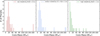 |
Fig. 4 Histograms showing the distribution of core masses for the planets in our sample. For low and medium atmospheric metallicities, the inferred core masses are mostly between 10 and 30 M⊕. The high log (Fe/H) retrievals produce lower core masses. Three large outliers can be seen with core masses >50 M⊕. |
4 Results
The derived envelope mass fractions of all the planets in our sample for the three log (Fe/H) cases are summarized in Table B.1. As expected, fenv is higher for larger log (Fe/H) values of a given planet. The total core masses of the planets are shown in Fig. 4. The low and medium log (Fe/H) cases show a similar distribution with most core masses between 10 and 30 M⊕. In the case of high log (Fe/H), the core mass distribution is shifted toward lower values (>10 M⊕).
In all three metallicity scenarios, there are three outliers of planets with unusually large core masses. These planets are TIC 139270665 b, Kepler-111 c, and Kepler-849 b. The masses of Kepler-111 c and Kepler-849 b reported in Dalba et al. (2024) have large uncertainties due to the long orbital period of the two planets and the relatively low number of available radial velocity observations. Additionally, as reported in Dalba et al. (2024), there are hints of further planets in the systems, which would influence the accuracy of the reported masses. None of the other planets in our sample exhibited significant RV variations from potentially undetected companions. Given the unreliable masses, we excluded both planets from the following analysis.
For TIC 139270665 b, we noticed the stellar radius derived in Peluso et al. (2024) is considerably smaller than in the TESS Input Catalogue (Paegert et al. 2022). Considering that the derived parallax for TIC 139270665 b (see Table 1 in Peluso et al. 2024) is significantly different from the Gaia DR3 value, we found that the ExoFAST modeling from Peluso et al. (2024) conflated the stellar input parameters with those of another star (Dalba & Peluso, priv. commun.). Therefore, the true stellar radius is likely larger than previously assumed, which would also increase the true radius of TIC 139270665 b. Updated modeling of the stellar and planetary parameters found a radius of 9.8 ± 0.5 R⊕ (Dalba & Peluso, priv. commun.). With this new radius, we ran a new set of retrievals for the planet.
Without Kepler-111 c and Kepler-849 b, we have a total of 26 planets with derived fenv for our analysis. The average uncertainty for fenv in our sample is 0.05, 0.07, and 0.05 for the low, medium, and high log (Fe/H) retrievals, respectively. We observed strong correlations between the percentage uncertainty of the radius and the error on the derived envelope mass fraction. We also find a correlation between the percentage uncertainty of the age and the associated fenv uncertainty, albeit weaker than the correlation with the radius uncertainty. Although the observed radius does not change much after 1 Gyr, as shown in Fig. 2, there is still a small slope for some of the models. As such, a larger age uncertainty increases the uncertainty of fenv. The mass uncertainty, on the other hand, showed only a weak correlation.
5 Discussion
5.1 fenv distribution of sub-Saturns
We compared the results from our interior modeling to a population of synthetic planets from the core-accretion model of Alessi et al. (2020). That model followed the semi-analytic formation model of (Ida & Lin 2004), which grows the planetary core through successive collisions of planetesimals from their underlying (assumed) smoothly distributed disk. The growing embryos gravitationally interact with their natal disk and migrate toward their host star throughout their formation, following the “planet trap” migration model (see Cridland et al. 2019, for details). When the influx of planetesimals is sufficiently small, the growing embryos begin to accrete a gaseous envelope. In that model, this transition occurs near a core mass of ∼ 5−10 M⊕; however, a few planets accreted cores of up to 50 M⊕ prior to the accretion of their gas2. To conform to the selected sample of this work, we limited the population of synthetic planets to the same period restriction as described above. Unlike the observed population, the synthetic planets are considered “young” and their interior structure is not computed (more below). Since we did not infer their physical size, only their mass and their fenv (derived directly from their accretion history) were compared.
For simplicity, their gas accretion rate is limited by a parameterized form of the Kelvin–Helmholtz timescale (see Ida & Lin 2004), with parameters that fit the numerical simulations of Ikoma et al. (2000). The functional form of the Kelvin–Helmholtz timescale used in Alessi et al. (2020) has τ ∝ M−2, so that when gas accretion first begins the accretion is slow (τ ∼ 0.5 Myr), but by the time the planetary embryo has grown to a Saturn-mass the accretion timescale has dropped to τ ∼ 5 kyr. While this parameterization captures the expected evolution of gas accretion, it does not explicitly handle the physical change (the envelope becoming self-gravitating) that is expected to cause the runaway accretion discussed here.
Figure 5 shows fenv as a function of the planetary mass for the synthetic population and our sample. In the low log (Fe/H) case, the envelope mass fractions in our sample are almost all significantly smaller than expected from the planet formation model for a given planet mass. The medium- and high-metallicity retrievals produce fenv that are more similar to what we see in the formation model. In the intermediate mass range (∼ 40−50 M⊕) the high log (Fe/H) retrievals produced the most similar fenv results. However, in the high log (Fe/H) case, some of the derived fenv for sub-Saturns with larger masses (∼ 60−100 M⊕) significantly exceed the values we expect from the formation model. Here, the medium log (Fe/H) results provide a better fit to the synthetic planets. This is consistent with observations of atmospheric metallicities from the solar system. For the gas-rich planets in the Solar System, we find a roughly linear decrease in atmospheric metallicity from Uranus and Neptune (log (Fe/H) ∼ 80 × solar) to Saturn (log (Fe/H) ∼ 10 × solar) and Jupiter (log (Fe/H) ∼ 2−3 × solar; Kreidberg et al. 2014). While there is some tentative evidence of such a trend in the exoplanet population, it has not been definitively confirmed (Thorngren et al. 2016; Welbanks et al. 2019; Ohno et al. 2025).
For the fraction of low-fenv sub-Saturns in our sample, even the high log (Fe/H) retrievals are not in agreement with the synthetic planet population. One potential explanation is that these planets have even higher atmospheric metallicities than what we modeled for here, which would shift their fenv to higher values, closer to the synthetic planets. Since most of the low fenv planets in our sample also have lower masses similar to those of Neptune and Uranus, it is possible that their log (Fe/H) exceeds the maximum of 50 × solar of our retrievals. Alternatively, given that the population of synthetic planets of Alessi et al. (2020) represents “young” planets that have just emerged from their natal protoplanetary disk, there could be mass loss mechanisms that reduce the envelope mass fraction of these planets over gigayear timescales. However, the envelope mass fraction of sub-Saturns is not expected to be significantly affected by photoevaporation, especially beyond 0.1 au (Chen & Rogers 2016; Millholland et al. 2020). To investigate the effect of photoevaporation on our sample, we followed the approach in Doyle et al. (2025). We calculated the photoevaporation mass-loss timescale, tm:
 (2)
where Menv is the mass of the envelope and Ṁenv is the mass-loss rate of the envelope calculated from Owen & Wu (2017):
(2)
where Menv is the mass of the envelope and Ṁenv is the mass-loss rate of the envelope calculated from Owen & Wu (2017):
 (3)
For the efficiency parameter (η), we assumed 0.1, and the highenergy flux was calculated using the relation from Jackson et al. (2012) L ≈ 10−3.5 L⊙(M*/M⊙). Planets with mass-loss timescales tm>100 Myr are assumed to be stable against photoevaporation. All of the planets in our sample have photo-evaporative timescales well above 1 Gyr, the lowest being Kepler-450 b with 26 Gyr. We therefore conclude that photoevaporation should not have a significant impact on the sub-Saturns in our sample.
(3)
For the efficiency parameter (η), we assumed 0.1, and the highenergy flux was calculated using the relation from Jackson et al. (2012) L ≈ 10−3.5 L⊙(M*/M⊙). Planets with mass-loss timescales tm>100 Myr are assumed to be stable against photoevaporation. All of the planets in our sample have photo-evaporative timescales well above 1 Gyr, the lowest being Kepler-450 b with 26 Gyr. We therefore conclude that photoevaporation should not have a significant impact on the sub-Saturns in our sample.
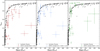 |
Fig. 5 Distribution of fenv as a function of planet mass for the sub-Saturns in our sample. We derived three different fenv for a low (left panel), medium (middle panel), and high (right panel) atmospheric metallicity case. The two planets with unreliable mass or radius measurements are indicated by the diamond markers. Black points are synthetic planets from the planetesimal accretion formation model of Alessi et al. (2020). The gray shaded area indicates planets with masses below the mass limit of our sample. The synthetic planets represent young planets at a time just after their natal disk has photo-evaporated. While they will contract their envelope over time, this does not affect the total mass and envelope mass fraction. |
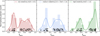 |
Fig. 6 Histograms showing the fenv distribution for low (left panel), medium (middle panel), and high (right panel) atmospheric metallicities. The black points at the bottom are the inferred fenv values of the planets in our sample (distributed in the y-axis direction for visibility). The solid lines show an estimation of the probability density of the fenv distribution using kernel density estimation. |
5.2 A runaway accretion gap?
Planets that start the process of runaway accretion will rapidly accumulate large amounts of gas. Assuming that runaway accretion starts when Mcore=Menv, there should be a paucity of planets with fenv ∼ 50% as these planets would have to have started runaway accretion at nearly the same time as their disk evaporated and thereby only gaining a small amount of gas in their envelopes after reaching fenv ∼ 50%. To investigate the existence of such a “runaway accretion gap,” we look at the distribution of fenv values in our sample. Figure 6 shows histograms of fenv for the three atmospheric metallicity cases. Together with the histograms, we plotted an estimate for the probability density function of the distribution using kernel density estimation. Kernel density estimation takes the measurement errors on the fenv values into account and convolves them with a bandwidth that is used to control the smoothness of the estimate. For all three distributions, we used a bandwidth of 0.05.
The three histograms have a bimodal distribution with a gap where no fenv values are found. The location of the gap depends on the assumed metallicity of the atmosphere. For low and medium log (Fe/H) atmospheres, the gap is between 0.3 and 0.5 fenv, with a slightly wider gap in the medium-metallicity case. The gap for the high log (Fe/H) retrievals is between 0.5 and 0.7 fenv. This is what would be expected for the fenv distribution after formation if runaway accretion starts at Mcore=Menv. In this case, the intermediate-sized planets could be divided into super-Neptunes (fenv<0.5) that did not start runaway accretion and sub-Saturns (fenv>0.7) that did.
Another parameter that might be relevant for runaway accretion is the hydrogen and helium mass fraction (fH/He). While fenv encompasses the whole mass of the atmosphere, including metals, fH/He only considers the mass of hydrogen and helium in the atmosphere. Venturini et al. (2016) computed self-consistent planet formation models including envelope enrichment and found that fH/He ∼ 30% at the onset of runaway accretion for multiple different initial conditions. However, they did not find an obvious explanation for why that would be happening in their models. Looking at the distribution of fH/He in our sample, we find a gap between fH/He values of 0.3 and 0.4 (see Fig. 7), seemingly corroborating the results in Venturini et al. (2016). While the exact shape of the distribution at higher fH/He changes, the position of the gap in fH/He at 0.3 is independent of the assumed atmospheric metallicity. There is a clear gap in the distribution of both fenv and fH/He. For both distributions, the same planets fall below and above the gap. This bimodal distribution, including a “runaway accretion gap,” is consistent with the model of core accretion, where runaway accretion is a rapid process that starts at fenv ∼ 0.5. However, the gaps in the distributions of fenv and fH/He could also stem from our limited sample size. As shown in Fig. 8, the gap in fenv coincides with a lack of planets in our sample with radii between 6.2 R⊕ and 7 R⊕. Given the strict selection criteria in our sample, we investigated whether this lack of planets exists in the wider exoplanet population. We still looked for mature, longer-period planets, as young or short-period planets could have radii in this range that are inflated, from either tides or internal heat, while still having low fenv below the gap. In the NASA Exoplanet Archive composite table, there are a total of 80 sub-Saturns when imposing the same conditions on radius precision, orbital period, and age as we did for our sample, but without the requirement of a measured mass. Out of these 80 sub-Saturns, seven are listed in the composite data with a radius between 6.2 R⊕ and 7 R⊕. However, updated values for KOI-94 e and TOI-1386 b place them below 6.2 R⊕. The lack of planets in this radius regime may therefore be a real feature caused by the onset of runaway accretion.
We also explored the impact of the age threshold on the distribution of fenv. Figure 8 (right) shows a stacked histogram of the derived fenv values assuming high log (Fe/H) for different age bins. We compared how the distribution would change if we restricted the sample to even older planets (above 3 Gyr within 1 σ). For this comparison, we also included high log (Fe/H) retrievals of the planets that were excluded after our age calculation because they were not older than 1 Gyr within 1 σ. As shown in the histograms and the probability density functions on top of the plot, the distribution does not change significantly for the different ages. The distribution is bimodal in all three cases, although it is less pronounced if the young planets are included. In particular, there are two planets (Kepler-30 d and TOI-1823 b with fenv between 0.6 and 0.7, narrowing the observed gap. However, given their young and uncertain age, the error bar on the derived fenv is quite large. Additionally, as discussed briefly in Sect. 2.2, the literature ages for these two planets are older than the age derived in this work. Without the internal heat from the young age that was assumed for the retrieval, the envelope mass fraction would be larger to account for the observed radii moving the planets to the right of the histogram, thus widening the fenv gap.
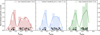 |
Fig. 7 Similar to Fig. 6 but showing the hydrogen and helium mass fraction (fH/He) distribution for low (left panel), medium (middle panel), and high (right panel) atmospheric metallicities. The black points at the bottom are the inferred fH/He values of the planets in our sample (distributed in the y-axis direction for visibility). |
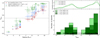 |
Fig. 8 Left: derived envelope mass fraction as a function of radius for the planets in our sample. The dotted black line marks the 50% fenv threshold. The gap in fenv for the different retrievals coincides with a gap in radius between 6.2 and 7 R⊕. Right: distribution of fenv as a histogram for different age thresholds. Planets are distributed in subsamples of planets older than 3 Gyr within 1 σ, planets older than 1 Gyr within 1 σ, and all planets initially considered for the sample before the age cutoff. On top are kernel density estimator functions based on the subsample. The bimodal shape of the distribution is independent of the age threshold. |
5.3 Differences between savanna sub-Saturns and desert and ridge sub-Saturns
Doyle et al. (2025) used GASTLI to analyze the envelope mass fractions of planets in the Neptune desert and ridge. In Fig. 9 we compare the fenv distribution of desert and ridge sub-Saturns from Doyle et al. (2025) to our longer-period sample. In their work, they assumed solar metallicity in the fenv retrievals, so to ensure comparability, we used our low log (Fe/H) sample. Additionally, we only included planets from Doyle et al. (2025) that would be sub-Saturns in our sample (i.e., 4 R⊕<Rp<8 R⊕). This removes the majority of planets in the Neptune desert, as these were mainly sub-Neptunes. The three sub-Saturns in the Neptune desert all have small envelope mass fractions. While this is expected for the two lower-mass planets, TOI-3071 b has an unusually low fenv given its mass of 68 ± 4 M⊕ (Hacker et al. 2024).
On the other hand, the distribution of fenv for sub-Saturns in the Neptunian ridge is similar to the distribution of our Neptunian savanna sample. To assess the similarity between the fenv distribution of the ridge sub-Saturns and our savanna sub-Saturns, we used a permutation test. Assuming that the two distributions come from the same underlying population, we partitioned the combined dataset randomly into two subsets corresponding to the original sizes of the two populations. We calculated the mean of the pairwise distance for 1000 permutations to compare with the observed distribution. Our test yields a p-value of 0.325, indicating no statistically significant difference between the two distributions. Our results indicate that there is no significant difference between the envelope mass fractions of sub-Saturns located in the Neptune ridge and those located in the Neptune savanna. Recent works have found potential differences in the density and host star metallicity between planets in the ridge and the savanna, pointing to different formation or evolution pathways of the two sub-Saturn populations (Castro-González et al. 2024b; Vissapragada & Behmard 2025). While our results appear to be in contrast to their findings, the small sample size of the ridge sub-Saturns, particularly in the higher fenv regime, makes it difficult to draw definitive conclusions.
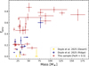 |
Fig. 9 Comparing the fenv of our low log (Fe/H) sample to the results from Doyle et al. (2025). We only include planets that satisfy the subSaturn definition used in the work. The Doyle et al. (2025) sample is separated into planets within the Neptune desert (P<3.2 d) and the ridge (3.2 d<P<6 d). |
6 Summary and conclusions
We derived the envelope mass fraction distribution of a sample of 28 warm sub-Saturns to compare with the outcomes from planet formation models. In particular, we investigated whether the onset of runaway accretion leaves an imprint on the population of sub-Saturns. We find that the exact distribution of fenv in our sample depends strongly on the assumed atmospheric metallicity for the planets. The best agreement with predictions from the planetesimal accretion model of Alessi et al. (2020) is produced assuming medium (0.5<log (Fe/H)<1.4) to high (log (Fe/H)>1.4) atmospheric metallicities.
Additionally, we find a bimodal distribution of fenv with a gap that could be caused by the onset of runaway accretion. This bimodality is seen for all three assumed atmospheric metallicities. However, the location of this gap is dependent on the atmospheric metallicity and only matches theoretical predictions for high log (Fe/H). This bimodality is also seen in the distribution of the hydrogen and helium mass fraction, fH/He. The gap in this distribution is located at 30%, corroborating the result from Venturini et al. (2016), which is yet to be explained. Lastly, when comparing the distribution of fenv for warm sub-Saturns in the Neptunian savanna to fenv measurements from Doyle et al. (2025) of hot sub-Saturns in the Neptune desert and ridge, we find no statistically significant difference between the savanna and ridge population.
We have shown tentative evidence of a gap in the sub-Saturn population that may be caused by runaway accretion. However, we are limited by the size of our sample and the absence of measurements of atmospheric log (Fe/H). Confirming more warm sub-Saturns (P>15 d) to expand the sample, particularly with radii between 6.2 and 7 R⊕, is key to further investigating the existence of a gap in the fenv distribution. Additionally, measuring the atmospheric metallicities of these sub-Saturns will be crucial to breaking the degeneracy between fenv and log (Fe/H) and deriving accurate envelope mass fractions. This is especially important when interpreting the fenv distribution in the context of planet formation models, such as linking the gap in fenv to runaway accretion.
The fenv is constant from subsolar log (Fe/H) to ∼ 10 × solar and increases rapidly for higher log (Fe/H). As such, knowing in which regime a planet falls can help improve the derived fenv even in the absence of extremely precise measurements. The results of an analysis like this can, in turn, inform planet formation models.
Data availability
The model grids that are used to perform the interior structure retrievals are made publicly available via Zenodo (https://zenodo.org/records/17396266).
Acknowledgements
We thank the anonymous referee for the corrections and suggestions that helped us improve the presentation of the paper. The authors thank Daniel Peluso, Paul Dalba, and Lauren Sgro for their input on the parameters of TIC 139270665 b, and Jan-Niklas Pippert for helpful discussions surrounding the paper. LT acknowledges support from the Excellence Cluster ORIGINS funded by the Deutsche Forschungsgemeinschaft (DFG, German Research Foundation) under Germany’s Excellence Strategy – EXC 2094 – 390783311. This research has made use of the NASA Exoplanet Archive, which is operated by the California Institute of Technology, under contract with the National Aeronautics and Space Administration under the Exoplanet Exploration Program.
References
- Abdurro’uf, Accetta K., Aerts, C., et al. 2022, ApJS, 259, 35 [NASA ADS] [CrossRef] [Google Scholar]
- Acuña, L., Deleuil, M., Mousis, O., et al. 2021, A&A, 647, A53 [NASA ADS] [CrossRef] [EDP Sciences] [Google Scholar]
- Acuña, L., Kreidberg, L., Zhai, M., & Mollière, P., 2024, A&A, 688, A60 [NASA ADS] [CrossRef] [EDP Sciences] [Google Scholar]
- Acuña, L., Kreidberg, L., Zhai, M., Mollière, P., & Fouesneau, M., 2025, J. Open Source Softw., 10, 7288 [Google Scholar]
- Alessi, M., Pudritz, R. E., & Cridland, A. J., 2020, MNRAS, 493, 1013 [NASA ADS] [CrossRef] [Google Scholar]
- Alibert, Y., 2017, A&A, 606, A69 [NASA ADS] [CrossRef] [EDP Sciences] [Google Scholar]
- Alibert, Y., Venturini, J., Helled, R., et al. 2018, Nat. Astron., 2, 873 [NASA ADS] [CrossRef] [Google Scholar]
- Angus, R., Morton, T., & Foreman-Mackey, D., 2019, J. Open Source Softw., 4, 1469 [NASA ADS] [CrossRef] [Google Scholar]
- Barragán, O., Gandolfi, D., Smith, A. M. S., et al. 2018, MNRAS, 475, 1765 [Google Scholar]
- Beaugé, C., & Nesvorný, D., 2013, ApJ, 763, 12 [Google Scholar]
- Bodenheimer, P., & Pollack, J. B., 1986, Icarus, 67, 391 [Google Scholar]
- Borsato, L., Malavolta, L., Piotto, G., et al. 2019, MNRAS, 484, 3233 [NASA ADS] [CrossRef] [Google Scholar]
- Bourrier, V., Attia, M., Mallonn, M., et al. 2023, A&A, 669, A63 [NASA ADS] [CrossRef] [EDP Sciences] [Google Scholar]
- Brady, M. T., Petigura, E. A., Knutson, H. A., et al. 2018, AJ, 156, 147 [NASA ADS] [CrossRef] [Google Scholar]
- Brewer, J. M., & Fischer, D. A., 2018, ApJS, 237, 38 [NASA ADS] [CrossRef] [Google Scholar]
- Brouwers, M. G., Vazan, A., & Ormel, C. W., 2018, A&A, 611, A65 [NASA ADS] [CrossRef] [EDP Sciences] [Google Scholar]
- Bruno, G., Almenara, J. M., Barros, S. C. C., et al. 2015, A&A, 573, A124 [NASA ADS] [CrossRef] [EDP Sciences] [Google Scholar]
- Buchhave, L. A., Bakos, G. Á., Hartman, J. D.,, et al. 2010, ApJ, 720, 1118 [NASA ADS] [CrossRef] [Google Scholar]
- Buchhave, L. A., Latham, D., Johansen, A., et al. 2012, Nature, 486, 375 [NASA ADS] [CrossRef] [Google Scholar]
- Castro-González, A., Bourrier, V., Lillo-Box, J., et al. 2024a, A&A, 689, A250 [NASA ADS] [CrossRef] [EDP Sciences] [Google Scholar]
- Castro-González, A., Lillo-Box, J., Armstrong, D. J., et al. 2024b, A&A, 691, A233 [NASA ADS] [CrossRef] [EDP Sciences] [Google Scholar]
- Chakraborty, A., Roy, A., Sharma, R., et al. 2018, AJ, 156, 3 [Google Scholar]
- Chen, H., & Rogers, L. A., 2016, ApJ, 831, 180 [Google Scholar]
- Chontos, A., Huber, D., Grunblatt, S. K., et al. 2024, arXiv e-prints [arXiv:2402.07893] [Google Scholar]
- Christiansen, J. L., McElroy, D. L., Harbut, M., et al. 2025, PSJ, 6, 186 [Google Scholar]
- Cridland, A. J., Pudritz, R. E., & Alessi, M., 2019, MNRAS, 484, 345 [Google Scholar]
- Cridland, A. J., van Dishoeck, E. F., Alessi, M., & Pudritz, R. E., 2020, A&A, 642, A229 [NASA ADS] [CrossRef] [EDP Sciences] [Google Scholar]
- Dalba, P. A., Gupta, A. F., Rodriguez, J. E., et al. 2020, AJ, 159, 241 [NASA ADS] [CrossRef] [Google Scholar]
- Dalba, P. A., Kane, S. R., Isaacson, H., et al. 2024, ApJS, 271, 16 [NASA ADS] [CrossRef] [Google Scholar]
- Danti, C., Bitsch, B., & Mah, J., 2023, A&A, 679, L7 [NASA ADS] [CrossRef] [EDP Sciences] [Google Scholar]
- Dawson, R. I., Huang, C. X., Lissauer, J. J., et al. 2019, AJ, 158, 65 [NASA ADS] [CrossRef] [Google Scholar]
- Dorn, C., Khan, A., Heng, K., et al. 2015, A&A, 577, A83 [NASA ADS] [CrossRef] [EDP Sciences] [Google Scholar]
- Doyle, L., Armstrong, D. J., Acuña, L., et al. 2025, MNRAS, 539, 3138 [Google Scholar]
- Dubber, S. C., Mortier, A., Rice, K., et al. 2019, MNRAS, 490, 5103 [NASA ADS] [CrossRef] [Google Scholar]
- Fabrycky, D. C., Ford, E. B., Steffen, J. H., et al. 2012, ApJ, 750, 114 [Google Scholar]
- Fűrész, G., 2008, PhD thesis, University of Szeged, Hungary [Google Scholar]
- Foreman-Mackey, D., Hogg, D. W., Lang, D., & Goodman, J., 2013, PASP, 125, 306 [Google Scholar]
- Gill, S., Wheatley, P. J., Cooke, B. F., et al. 2020, ApJ, 898, L11 [Google Scholar]
- Gill, S., Bayliss, D., Ulmer-Moll, S., et al. 2024, MNRAS, 533, 109 [Google Scholar]
- Ginzburg, S., Schlichting, H. E., & Sari, R., 2016, ApJ, 825, 29 [Google Scholar]
- Grimm, S. L., Demory, B.-O., Gillon, M., et al. 2018, A&A, 613, A68 [NASA ADS] [CrossRef] [EDP Sciences] [Google Scholar]
- Guillot, T., & Gautier, D., 2015, in Treatise on Geophysics, ed. G. Schubert, 529 [Google Scholar]
- Hacker, A., Díaz, R. F., Armstrong, D. J., et al. 2024, MNRAS, 532, 1612 [NASA ADS] [CrossRef] [Google Scholar]
- Hartman, J. D., Bakos, G. Á., Torres, G.,, et al. 2009, ApJ, 706, 785 [NASA ADS] [CrossRef] [Google Scholar]
- Helled, R., 2023, A&A, 675, L8 [NASA ADS] [CrossRef] [EDP Sciences] [Google Scholar]
- Hill, M. L., Kane, S. R., Dalba, P. A., et al. 2024, AJ, 167, 151 [Google Scholar]
- Hori, Y., & Ikoma, M., 2011, MNRAS, 416, 1419 [NASA ADS] [CrossRef] [Google Scholar]
- Ida, S., & Lin, D. N. C., 2004, ApJ, 604, 388 [Google Scholar]
- Ikoma, M., Nakazawa, K., & Emori, H., 2000, ApJ, 537, 1013 [NASA ADS] [CrossRef] [Google Scholar]
- Irwin, P. G. J., Lellouch, E., de Bergh, C., et al. 2014, Icarus, 227, 37 [Google Scholar]
- Jackson, A. P., Davis, T. A., & Wheatley, P. J., 2012, MNRAS, 422, 2024 [Google Scholar]
- Jackson, B., Arras, P., Penev, K., Peacock, S., & Marchant, P., 2017, ApJ, 835, 145 [NASA ADS] [CrossRef] [Google Scholar]
- Jontof-Hutter, D., Dalba, P. A., & Livingston, J. H., 2022, AJ, 164, 42 [NASA ADS] [CrossRef] [Google Scholar]
- König, P. C., Damasso, M., Hébrard, G., et al. 2022, A&A, 666, A183 [NASA ADS] [CrossRef] [EDP Sciences] [Google Scholar]
- Koskinen, T. T., Lavvas, P., Huang, C., et al. 2022, ApJ, 929, 52 [NASA ADS] [CrossRef] [Google Scholar]
- Kreidberg, L., Bean, J. L., Désert, J.-M.,, et al. 2014, ApJ, 793, L27 [Google Scholar]
- Kunimoto, M., Vanderburg, A., Huang, C. X., et al. 2023, AJ, 166, 7 [NASA ADS] [CrossRef] [Google Scholar]
- Kurokawa, H., & Nakamoto, T., 2014, ApJ, 783, 54 [NASA ADS] [CrossRef] [Google Scholar]
- Kurucz, R. L., 1992, in The Stellar Populations of Galaxies, 149, eds. B. Barbuy, & A. Renzini, 225 [NASA ADS] [CrossRef] [Google Scholar]
- Lecavelier Des Etangs, A., 2007, A&A, 461, 1185 [NASA ADS] [CrossRef] [EDP Sciences] [Google Scholar]
- Lee, E. J., & Chiang, E., 2015, ApJ, 811, 41 [Google Scholar]
- Lee, E. J., Chiang, E., & Ormel, C. W., 2014, ApJ, 797, 95 [Google Scholar]
- Lissauer, J. J., 1993, ARA&A, 31, 129 [NASA ADS] [CrossRef] [Google Scholar]
- Lopez, E. D., & Fortney, J. J., 2014, ApJ, 792, 1 [Google Scholar]
- Lozovsky, M., Helled, R., Rosenberg, E. D., & Bodenheimer, P., 2017, ApJ, 836, 227 [NASA ADS] [CrossRef] [Google Scholar]
- Lundkvist, M. S., Kjeldsen, H., Albrecht, S., et al. 2016, Nat. Commun., 7, 11201 [Google Scholar]
- MacDonald, R. J., & Madhusudhan, N., 2019, MNRAS, 486, 1292 [Google Scholar]
- MacDougall, M. G., Petigura, E. A., Gilbert, G. J., et al. 2023, AJ, 166, 33 [NASA ADS] [CrossRef] [Google Scholar]
- Mancini, L., Lillo-Box, J., Southworth, J., et al. 2016, A&A, 590, A112 [NASA ADS] [CrossRef] [EDP Sciences] [Google Scholar]
- Matsakos, T., & Königl, A., 2016, ApJ, 820, L8 [Google Scholar]
- Mazeh, T., Holczer, T., & Faigler, S., 2016, A&A, 589, A75 [NASA ADS] [CrossRef] [EDP Sciences] [Google Scholar]
- Miguel, Y., & Vazan, A., 2023, Remote Sensing, 15, 681 [NASA ADS] [CrossRef] [Google Scholar]
- Millholland, S., Petigura, E., & Batygin, K., 2020, ApJ, 897, 7 [NASA ADS] [CrossRef] [Google Scholar]
- Mistry, P., Pathak, K., Lekkas, G., et al. 2023, MNRAS, 521, 1066 [NASA ADS] [CrossRef] [Google Scholar]
- Mizuno, H., 1980, Prog. Theoret. Phys., 64, 544 [NASA ADS] [CrossRef] [Google Scholar]
- Mizuno, H., Nakazawa, K., & Hayashi, C., 1978, Prog. Theoret. Phys., 60, 699 [Google Scholar]
- Mollière, P., van Boekel, R., Dullemond, C., Henning, T., & Mordasini, C., 2015, ApJ, 813, 47 [Google Scholar]
- Mollière, P., van Boekel, R., Bouwman, J., et al. 2017, A&A, 600, A10 [Google Scholar]
- Mordasini, C., Alibert, Y., & Benz, W., 2009, A&A, 501, 1139 [CrossRef] [EDP Sciences] [Google Scholar]
- Müller, S., & Helled, R., 2023, A&A, 669, A24 [NASA ADS] [CrossRef] [EDP Sciences] [Google Scholar]
- Nascimbeni, V., Borsato, L., Leonardi, P., et al. 2024, A&A, 690, A349 [NASA ADS] [CrossRef] [EDP Sciences] [Google Scholar]
- Nowak, G., Palle, E., Gandolfi, D., et al. 2020, MNRAS, 497, 4423 [NASA ADS] [CrossRef] [Google Scholar]
- Ohno, K., Ikoma, M., Okuzumi, S., & Kimura, T., 2025, arXiv e-prints, [arXiv:2506.16060] [Google Scholar]
- Owen, J. E., 2019, Annu. Rev. Earth Planet. Sci., 47, 67 [CrossRef] [Google Scholar]
- Owen, J. E., & Wu, Y., 2017, ApJ, 847, 29 [Google Scholar]
- Owen, J. E., & Lai, D., 2018, MNRAS, 479, 5012 [Google Scholar]
- Paegert, M., Stassun, K. G., Collins, K. A., et al. 2022, VizieR Online Data Catalog: TESS Input Catalog version 8.2 (TIC v8.2) (Paegert+, 2021), VizieR On-line Data Catalog: IV/39. Originally published in: 2021arXiv210804778P [Google Scholar]
- Peluso, D. O., Dalba, P. A., Wright, D., et al. 2024, AJ, 167, 170 [Google Scholar]
- Perri, F., & Cameron, A. G. W., 1974, Icarus, 22, 416 [Google Scholar]
- Petigura, E. A., Howard, A. W., Lopez, E. D., et al. 2016, ApJ, 818, 36 [Google Scholar]
- Petigura, E. A., Sinukoff, E., Lopez, E. D., et al. 2017, AJ, 153, 142 [NASA ADS] [CrossRef] [Google Scholar]
- Petigura, E. A., Benneke, B., Batygin, K., et al. 2018, AJ, 156, 89 [Google Scholar]
- Petigura, E. A., Livingston, J., Batygin, K., et al. 2020, AJ, 159, 2 [NASA ADS] [CrossRef] [Google Scholar]
- Petigura, E. A., Rogers, J. G., Isaacson, H., et al. 2022, AJ, 163, 179 [NASA ADS] [CrossRef] [Google Scholar]
- Polanski, A. S., Lubin, J., Beard, C., et al. 2024, ApJS, 272, 32 [NASA ADS] [CrossRef] [Google Scholar]
- Pollack, J. B., Podolak, M., Bodenheimer, P., & Christofferson, B., 1986, Icarus, 67, 409 [Google Scholar]
- Pollack, J. B., Hubickyj, O., Bodenheimer, P., et al. 1996, Icarus, 124, 62 [NASA ADS] [CrossRef] [Google Scholar]
- Rainer, M., Desidera, S., Borsa, F., et al. 2023, A&A, 676, A90 [NASA ADS] [CrossRef] [EDP Sciences] [Google Scholar]
- Rescigno, F., Hébrard, G., Vanderburg, A., et al. 2024, MNRAS, 527, 5385 [Google Scholar]
- Rodríguez Martínez, R., Eastman, J. D., Collins, K. A., et al. 2025, AJ, 169, 72 [Google Scholar]
- Sanchis-Ojeda, R., Rappaport, S., Winn, J. N., et al. 2014, ApJ, 787, 47 [Google Scholar]
- Sharma, S., Stello, D., Buder, S., et al. 2018, MNRAS, 473, 2004 [NASA ADS] [CrossRef] [Google Scholar]
- Stassun, K. G., Oelkers, R. J., Paegert, M., et al. 2019, AJ, 158, 138 [Google Scholar]
- Stevenson, D. J., 1982, Planet. Space Sci., 30, 755 [NASA ADS] [CrossRef] [Google Scholar]
- Szabó, G. M., & Kiss, L. L., 2011, ApJ, 727, L44 [Google Scholar]
- Tala Pinto, M., Jordán, A., Acuña, L., et al. 2025, A&A, 694, A268 [NASA ADS] [CrossRef] [EDP Sciences] [Google Scholar]
- Thomas, L., Hébrard, G., Kellermann, H., et al. 2025, A&A, 694, A143 [NASA ADS] [CrossRef] [EDP Sciences] [Google Scholar]
- Thorngren, D. P., Fortney, J. J., Murray-Clay, R. A., & Lopez, E. D., 2016, ApJ, 831, 64 [NASA ADS] [CrossRef] [Google Scholar]
- Trifonov, T., Brahm, R., Jordán, A., et al. 2023, AJ, 165, 179 [NASA ADS] [CrossRef] [Google Scholar]
- Udry, S., Mayor, M., & Santos, N. C., 2003, A&A, 407, 369 [NASA ADS] [CrossRef] [EDP Sciences] [Google Scholar]
- Ulmer-Moll, S., Osborn, H. P., Tuson, A., et al. 2023, A&A, 674, A43 [NASA ADS] [CrossRef] [EDP Sciences] [Google Scholar]
- Valletta, C., & Helled, R., 2020, in European Planetary Science Congress, EPSC2020–648 [Google Scholar]
- Venturini, J., & Helled, R., 2020, A&A, 634, A31 [NASA ADS] [CrossRef] [EDP Sciences] [Google Scholar]
- Venturini, J., Alibert, Y., & Benz, W., 2016, A&A, 596, A90 [NASA ADS] [CrossRef] [EDP Sciences] [Google Scholar]
- Vissapragada, S., & Behmard, A., 2025, AJ, 169, 117 [Google Scholar]
- Vissapragada, S., Jontof-Hutter, D., Shporer, A., et al. 2020, AJ, 159, 108 [NASA ADS] [CrossRef] [Google Scholar]
- Vissapragada, S., Knutson, H. A., Greklek-McKeon, M., et al. 2022, AJ, 164, 234 [NASA ADS] [CrossRef] [Google Scholar]
- Wakeford, H. R., Sing, D. K., Deming, D., et al. 2018, AJ, 155, 29 [Google Scholar]
- Welbanks, L., Madhusudhan, N., Allard, N. F., et al. 2019, ApJ, 887, L20 [NASA ADS] [CrossRef] [Google Scholar]
- Yahalomi, D. A., Kipping, D., Nesvorný, D., et al. 2024, MNRAS, 527, 620 [Google Scholar]
- Yoffe, G., Ofir, A., & Aharonson, O., 2021, ApJ, 908, 114 [NASA ADS] [CrossRef] [Google Scholar]
The precise core mass for initiating gas accretion depends on the choice of a threshold planetesimal accretion rate of one M⊕ per Myr, based on the results of Ikoma et al. (2000).
Appendix A stardate results
Input properties and ages from the stardate modeling of host stars.
Appendix B GASTLI results
Properties and results of the interior structure modeling for the planets in our sample.
All Tables
Properties and results of the interior structure modeling for the planets in our sample.
All Figures
|
Fig. 1 Mass-radius diagram of the sub-Saturns in our sample. The colored points show the exoplanet population with radii and masses measured to the precision of our selection criteria. Their colors indicate the orbital periods of the planets. The sub-Saturns that were analyzed in this work are overplotted in black. |
| In the text | |
|
Fig. 2 Thermal evolution curves for a planet with a CMF of 0.35 and a mass of 0.2 MJ with varying atmospheric metallicities. The input internal temperatures are converted to ages, and the planet radius at each step is calculated by GASTLI. A higher assumed atmospheric metallicity leads to a lower total radius. After ∼ 1 Gyr, the change in radius due to the contraction of the planetary envelope is small even for low-metallicity atmospheres. |
| In the text | |
|
Fig. 3 Corner plots of the interior structure retrieval for Kepler-280b. Shown in black is the retrieval without any constraint on log (Fe/H). While the CMF is uncorrelated for the majority of log (Fe/H) values, for high atmospheric metallicities the inferred CMF decreases significantly. To illustrate this, the contours for low (−2.0<log (Fe/H)<0.5), medium (0.5<log (Fe/H)≤1.4), and high (1.4<log (Fe/H)<1.7) atmospheric metallicity retrievals are overplotted in red, blue, and green, respectively. |
| In the text | |
|
Fig. 4 Histograms showing the distribution of core masses for the planets in our sample. For low and medium atmospheric metallicities, the inferred core masses are mostly between 10 and 30 M⊕. The high log (Fe/H) retrievals produce lower core masses. Three large outliers can be seen with core masses >50 M⊕. |
| In the text | |
|
Fig. 5 Distribution of fenv as a function of planet mass for the sub-Saturns in our sample. We derived three different fenv for a low (left panel), medium (middle panel), and high (right panel) atmospheric metallicity case. The two planets with unreliable mass or radius measurements are indicated by the diamond markers. Black points are synthetic planets from the planetesimal accretion formation model of Alessi et al. (2020). The gray shaded area indicates planets with masses below the mass limit of our sample. The synthetic planets represent young planets at a time just after their natal disk has photo-evaporated. While they will contract their envelope over time, this does not affect the total mass and envelope mass fraction. |
| In the text | |
|
Fig. 6 Histograms showing the fenv distribution for low (left panel), medium (middle panel), and high (right panel) atmospheric metallicities. The black points at the bottom are the inferred fenv values of the planets in our sample (distributed in the y-axis direction for visibility). The solid lines show an estimation of the probability density of the fenv distribution using kernel density estimation. |
| In the text | |
|
Fig. 7 Similar to Fig. 6 but showing the hydrogen and helium mass fraction (fH/He) distribution for low (left panel), medium (middle panel), and high (right panel) atmospheric metallicities. The black points at the bottom are the inferred fH/He values of the planets in our sample (distributed in the y-axis direction for visibility). |
| In the text | |
|
Fig. 8 Left: derived envelope mass fraction as a function of radius for the planets in our sample. The dotted black line marks the 50% fenv threshold. The gap in fenv for the different retrievals coincides with a gap in radius between 6.2 and 7 R⊕. Right: distribution of fenv as a histogram for different age thresholds. Planets are distributed in subsamples of planets older than 3 Gyr within 1 σ, planets older than 1 Gyr within 1 σ, and all planets initially considered for the sample before the age cutoff. On top are kernel density estimator functions based on the subsample. The bimodal shape of the distribution is independent of the age threshold. |
| In the text | |
|
Fig. 9 Comparing the fenv of our low log (Fe/H) sample to the results from Doyle et al. (2025). We only include planets that satisfy the subSaturn definition used in the work. The Doyle et al. (2025) sample is separated into planets within the Neptune desert (P<3.2 d) and the ridge (3.2 d<P<6 d). |
| In the text | |
Current usage metrics show cumulative count of Article Views (full-text article views including HTML views, PDF and ePub downloads, according to the available data) and Abstracts Views on Vision4Press platform.
Data correspond to usage on the plateform after 2015. The current usage metrics is available 48-96 hours after online publication and is updated daily on week days.
Initial download of the metrics may take a while.