| Issue |
A&A
Volume 703, November 2025
|
|
|---|---|---|
| Article Number | A35 | |
| Number of page(s) | 12 | |
| Section | The Sun and the Heliosphere | |
| DOI | https://doi.org/10.1051/0004-6361/202556728 | |
| Published online | 04 November 2025 | |
The solar sulphur abundance in view of large-scale atomic structure calculations and 3D non-LTE models
1
Theoretical Astrophysics, Department of Physics and Astronomy, Uppsala University, Box 516 SE-751 20 Uppsala, Sweden
2
National Astronomical Observatories, Chinese Academy of Sciences, Beijing 100012, PR China
3
Centre Spatial de Liège, Université de Liège, avenue Pré Aily, B-4031 Angleur-Liège, Belgium
4
Space sciences, Technologies and Astrophysics Research (STAR) Institute, Université de Liège, Allée du 6 août, 17, B5C, B-4000 Liège, Belgium
5
Busek Center for Meteorite Studies, Arizona State University, Tempe, Arizona 85287-6004, USA
6
Department of Earth Sciences, Dartmouth College, Hanover, New Hampshire 03755, USA
⋆ Corresponding author: This email address is being protected from spambots. You need JavaScript enabled to view it.
Received:
3
August
2025
Accepted:
5
September
2025
Abstract
The solar chemical composition is a fundamental yardstick in astrophysics and the topic of heated debate in recent literature. We re-evaluated the abundance of sulphur in the photosphere by studying seven S I lines in the solar disc-centre intensity spectrum. Our analysis considers independent sets of experimental and theoretical oscillator strengths together with, for the first time, three-dimensional non-local thermodynamic equilibrium (3D non-LTE) S I spectrum synthesis. Our best estimate is A(S) = 7.06 ± 0.04, which is 0.06 − 0.10 dex lower than that in commonly used compilations of the solar chemical composition. Our lower solar sulphur abundance deviates from that in CI chondrites and thereby supports the case for a systematic difference between the composition of the solar photosphere and of CI chondrites that is correlated with 50% condensation temperature. We suggest that precise laboratory measurements of S I oscillator strengths and abundance analyses using 3D magnetohydrodynamic models of the solar photosphere be conducted to further substantiate our conclusions.
Key words: atomic data / atomic processes / line: formation / radiative transfer / Sun: abundances / Sun: photosphere
© The Authors 2025
 Open Access article, published by EDP Sciences, under the terms of the Creative Commons Attribution License (https://creativecommons.org/licenses/by/4.0), which permits unrestricted use, distribution, and reproduction in any medium, provided the original work is properly cited.
This article is published in open access under the Subscribe to Open model. This email address is being protected from spambots. You need JavaScript enabled to view it. to support open access publication.
1. Introduction
The solar chemical composition is a fundamental yardstick in astrophysics, against which other cosmic objects are most often compared (e.g. Grevesse & Sauval 1998; Asplund et al. 2021). In this context, there is great interest in precise constraints on the solar sulphur abundance. Sulphur is an α element and thus interesting as a tracer of star formation in different stellar populations in the Milky Way (e.g. Perdigon et al. 2021; Lucertini et al. 2022, 2023) and in other galaxies (e.g. Dors et al. 2023; Goswami et al. 2024; Pérez-Montero et al. 2025). Additionally, sulphur has diagnostic power for studying gas-dust fractionation processes in protoplanetary discs around young stars (e.g. Kama et al. 2019; Keyte et al. 2024) and in circumbinary discs around evolved stars (e.g. Mohorian et al. 2025a,b). Sulphur is also relevant for studying the Sun itself. Within the Sun, sulphur is a non-negligible contributor to the opacity in the radiative zone (see Figure 2 of Buldgen et al. 2025). Thus sulphur may have a role in the long-debated solar-modelling problem (e.g. Christensen-Dalsgaard 2021). Sulphur may also be interesting for studies of the upper solar atmosphere. As an element of intermediate first ionisation potential (FIP; Eion = 10.36 eV), sulphur behaves as a high-FIP element in the closed-loop solar corona and as a low-FIP element in the solar wind, and this can help shed light on the fractionation physics (Laming et al. 2019).
In particular, recent analyses have put the spotlight on systematic differences between the solar photospheric composition and the abundances inferred from CI chondrites (e.g. Gonzalez et al. 2010; Asplund et al. 2021; Jurewicz et al. 2024). Namely, either refractory elements (with 50% having a condensation temperature of Tcond ≳ 1200 K) are depleted in CI chondrites, or moderately volatile elements (400 ≲ Tcond ≲ 1200 K) are enhanced in CI chondrites, compared to the photosphere, by up to around 20%. The measurements cannot constrain between these two scenarios (enrichment versus depletion) because that information is lost by converting the CI abundances to the solar scale, which in this work was done by setting A(Si) = 7.511 from Asplund et al. (2021). Nevertheless, these systematic differences call into question the assumption that CI chondrites are a precise reflection of the composition the protosolar nebula; moreover, the degree of depletion may help constrain models of how the Solar System formed (Desch et al. 2018). Sulphur is a key element in this discussion as it is a moderately volatile element (Tcond = 672 K; Wood et al. 2019). There are only a few elements with such low Tcond that have precise photospheric abundance measurements; in the critical compilation of Asplund et al. (2021), sulphur has the lowest nominal error bar of just 0.03 dex. Thus, systematic errors in the solar sulphur abundance could have a disproportionate effect on the systematic differences between the solar photospheric composition and CI chondrites, after taking the stipulated uncertainties into account.
The solar sulphur abundance from Asplund et al. (2021), A(S) = 7.12 ± 0.03, comes from the analysis of Scott et al. (2015). This was based on spectrum synthesis of eight S I lines with the code Scate (Hayek et al. 2011) using a three-dimensional (3D) radiation-hydrodynamics simulation of the solar photosphere with the code Stagger (Collet et al. 2018; Stein et al. 2024). They compared synthetic equivalent widths against measurements of solar-disc-centre intensity atlases (Delbouille et al. 1973; Neckel & Labs 1984) to obtain 3D local thermodynamic equilibrium (LTE) abundances. To correct for departures from LTE, the authors calculated 1D non-LTE versus 1D LTE abundance corrections using the model of Takeda et al. (2005) to obtain the final 3D LTE + 1D non-LTE result.
The purpose of this study is to revisit the solar sulphur abundance with consideration for two possible sources of systematic error in the analysis of Scott et al. (2015). The first of these is the treatment of departures from LTE; specifically, Scott et al. (2015) carried out an inconsistent 3D LTE + 1D non-LTE analysis, and employed a now outdated non-LTE model atom employing the antiquated Drawin recipe for inelastic collisions with neutral hydrogen (see Barklem et al. 2011 for a discussion of this topic). We carried out a consistent 3D non-LTE analysis based on a carefully constructed model atom that uses modern atomic data. The second possible source of systematic error is the set of oscillator strengths for the diagnostic S I lines; five of their eight S I lines do not have precise laboratory measurements, and thus the analysis of these lines is based on theoretical data. Here, we consider three independent sets of atomic structure calculations, including new calculations from Li et al. (2025), to demonstrate that there are significant systematic uncertainties in the atomic data. Ultimately, we argue that the solar sulphur abundance in Asplund et al. (2021) is overestimated and advocate for A(S) = 7.06 ± 0.04.
2. Method
2.1. Model atmosphere and spectrum synthesis
The synthetic spectra were calculated by post-processing radiative-transfer calculations of snapshots of a 3D radiation-hydrodynamics simulation of the solar photosphere. This model atmosphere was calculated using the code Stagger (Collet et al. 2018; Stein et al. 2024) with a resolution that is comparable to that of the Stagger-grid (Magic et al. 2013), but spanning around a day of solar time. It is the same model that has been used in our ongoing series of papers on the solar chemical composition beginning with Amarsi et al. (2018a) (see Amarsi et al. 2024, and references therein).
The post-processing calculations were performed using the 3D LTE code Scate (Hayek et al. 2011) and the 3D non-LTE code Balder (Amarsi et al. 2018b); the latter is a modified version of Multi3D (Leenaarts & Carlsson 2009). The model atom used by Balder is described in Section . For both sets of calculations, the model atmosphere was down-sampled in the two horizontal dimensions by a factor of 32 and refined in the vertical for better sampling of the layers with steep temperature gradient where the continuum photons escape (Rodríguez Díaz et al. 2024). The 3D non-LTE calculations using the Balder code were carried out on eight snapshots of the 3D model atmosphere. For each snapshot, five different values of sulphur abundances in steps of 0.2 dex were used, and the mean radiation field was calculated using the 26 – ray angle quadrature that is described in Amarsi et al. (2024). Background line opacities were pre-computed using the code Blue (Zhou et al. 2023). The 3D-non-LTE-to-3D-LTE-intensity ratios were computed and applied to 3D LTE intensities calculated with Scate. These latter calculations were performed with finer temporal and abundance resolution, namely 17 snapshots and 11 sulphur abundances using steps of 0.05 dex. The total and continuous spectra were averaged across these multiple snapshot and then continuum-normalised.
To quantify the 3D effects (e.g. the 3D non-LTE versus 1D non-LTE abundance differences), post-processing calculations with the Scate and Balder codes were also performed on a 1D model atmosphere. This model was calculated with the same equation of state and treatment of opacities as the 3D model, but with convection now described via mixing-length theory (such ATMO models are described in the appendix of Magic et al. 2013). In the 1D case, the synthetic spectra were calculated assuming a depth-independent microturbulence of ξ1D = 1 km s−1. This fudge parameter accounts for broadening caused by velocity gradients in the stellar atmosphere on scales much smaller than one optical depth. These gradients are not predicted by 1D models, but they naturally emerge in the 3D simulations (e.g. Nordlund et al. 2009). Thus, no microturbulence or other free parameters (apart from the sulphur abundance) were employed in the 3D LTE or 3D non-LTE spectrum syntheses.
We illustrate the temperature-τ relations of the 3D and 1D models in Figure 1. Comparisons with other 1D models and a horizontally and temporally averaged 3D model can be found in Figure 2 of Amarsi et al. (2021), for example.
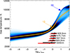 |
Fig. 1. Gas-temperature distribution with vertical logarithmic optical depth in the 3D model atmosphere (blue). The T − log τ relation of the corresponding 1D model atmosphere is also shown (orange). The full widths at half maximum of the line-profile’s integrated, 1D, non-LTE contribution functions to the line depressions (Amarsi 2015) are shown for the diagnostic S I lines (the line-averaged result is shown for the S I 1045 nm triplet). These are presented for both the disc-centre intensity (black) and disc-integrated flux (red) with circles indicating the positions of the peaks. |
2.2. Model atom
We illustrate the levels and lines of the comprehensive and reduced models in Figure 2, and we describe their construction below. The same models were recently used in Mohorian et al. (2025a, b) and Carlos et al. (2025); an early version was used in Kochukhov et al. (2024).
A comprehensive model atom was constructed for neutral sulphur using fine structure levels (namely, resolving L, S, and J; hereafter LSJ) up to E = 9.93 eV from Martin et al. (1990). These data were extracted from the NIST Database (Ralchenko & Kramida 2020) prior to the recent update of Civiš et al. (2024). The fine structure energies for the 5d 5Do, 7p 5P, and 6d 5Do terms were updated using the Kurucz database (Kurucz 1995). Higher LS terms were included from The Opacity Project (Cunto & Mendoza 1992; Seaton 1995), converting the reported quantum defects and experimental ionisation limits into energies relative to the ground state as described in Amarsi & Asplund (2017). Since the ionisation energy of sulphur is high (10.36 eV), neutral sulphur is the majority species, and so only the four lowest LS terms of singly ionised sulphur (taken from the NIST database and collapsed) were included in the model. Overall, the comprehensive model has 146 LSJ levels or LS terms, 142 of which are of neutral sulphur. Without any fine structure this would drop to 84 LS terms, comparable in complexity to the model presented in Korotin & Kiselev (2024), which contains 64 LS terms of neutral sulphur.
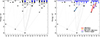 |
Fig. 2. Grotrian diagram for comprehensive (left) and reduced (right) model atoms used in this work. Terms for which fine-structure are unresolved are shown as short blue horizontal lines. Super levels in the reduced model atom are shown as long, blue horizontal lines. Transitions are shown as slanted grey lines; those used as abundance diagnostics are shown as coloured slanted lines in the right panel and labelled in the legend. |
The bound-bound radiative transitions were mainly taken from Podobedova et al. (2009) via the NIST database, most of which are based on Zatsarinny & Bartschat (2006). These were supplemented with data from The Opacity Project; where necessary, these LS data were redistributed across the LSJ levels using the tables in Allen (1973) to ensure a realistic description of the radiation field and thus the radiative rates for bound-bound transitions. With this combined data set in hand, natural broadening parameters were calculated by summations of the Einstein A coefficients, and Stark broadening parameters were extracted from the Kurucz database. Hydrogen collision broadening parameters were determined by interpolating the extended tables2 of Anstee & O’Mara (1995), Barklem & O’Mara (1997), and Barklem et al. (1998); when the line parameters were outside of these grids, the classical Unsöld recipe was used instead, with an enhancement factor of 2.0. The bound-free radiative transitions were taken from The Opacity Project; we took care to connect the neutral sulphur levels to the correct ionic core, shifting the provided wavelength basis such that the threshold wavelengths were consistent with the experimental energies from the NIST Database and (following Bard & Carlsson 2008) smoothing the sharp resonances in the data using a Gaussian filter.
For the collisions, the data for excitation by electron impact were mainly taken from OpenADAS (Summers & O’Mullane 2011), file ls#s0.dat. Missing allowed transitions were supplemented with calculations based on the recipe of Seaton (1962). Missing forbidden transitions were crudely estimated using the recipe of van Regemorter (1962), taking gf = 10−3; our tests found that these transitions had a negligible impact on the statistical equilibrium. The data for ionisation by electron impact were estimated using the recipe of Allen (1973). Excitation by neutral hydrogen impact as well as charge transfer involving different excited levels of neutral sulphur (S + H ↔ S+ + H−) were taken from the asymptotic model calculations of Belyaev & Voronov (2020). Motivated by Amarsi et al. (2018a) and subsequent studies, the rate coefficients for excitation were added to those calculated using the free-electron model (in the scattering-length approximation) of Kaulakys (1985, 1986, 1991). The free-electron model was also used to estimate the rate of ionisation by hydrogen impact. The collisional data described above do not consider fine structure; thus, the rate coefficients within LS terms were set to very high values, while the rate coefficients between LS terms were redistributed to the LSJ structure of the model atom so as to approximately conserve the total rates (e.g. Caliskan et al. 2025). Test 1D non-LTE calculations using a model atom with rate coefficients perturbed by a factor of ten showed that the statistical equilibrium is overall most sensitive to the excitation by neutral hydrogen impact, followed by excitation and then by electron impact. Moreover, the S I 1045 nm triplet, which shows large departures from LTE, is mainly sensitive to the collisions that couple its own lower and upper levels.
To reduce the computational cost, a 66 – level reduced model atom was constructed. Fine-structure LSJ levels were collapsed into LS terms for levels above 8.8 eV, and LS terms above 9.93 eV of the same multiplicity and within ±0.05 eV were merged into so-called super levels. There are seven super levels in total, with the highest one just 0.15 eV below the first ionisation limit. The affected transitions were collapsed into super transitions following the approaches described in Lind & Amarsi (2024). Testing 1D non-LTE calculations showed that the departure coefficients of the comprehensive and reduced model atoms closely follow each other, such that the abundance corrections for both the disc-centre intensity and disc-integrated flux agree between the two models to 0.001 dex in the worst case. For the production runs, the non-LTE iterations were performed on the reduced model to determine departure coefficients for each LSJ level, LS term, or super level. The final emergent spectra were calculated after applying these departure coefficients onto the LTE populations of the corresponding LSJ levels or LS terms in the comprehensive model.
2.3. Diagnostic S I lines and oscillator strengths
The focus of this work is on seven S I lines, a subset of the eight lines studied in Scott et al. (2015). The S I 469.41 nm that was included in their study is omitted here because of difficulties in accurately placing the continuum corresponding to a large uncertainty in equivalent width. We highlight the seven S I lines in Figure 2 and illustrate their formation regions in Figure 1. We also list the key line parameters in Table 1. As the S I 675 nm triplet is modelled with fine structure, there are nine lines shown in the table.
Parameters for diagnostic S I lines.
Four sets of oscillator strengths are considered in this analysis and are listed in different columns of Table 1. First are the experimental data of Zerne et al. (1997), which are only available for the S I 1045 nm triplet. These are based on laboratory lifetime measurements using laser spectroscopy. The reported uncertainties are only of the order of ±0.01 dex.
The other three data sets are based on mid-scale or large-scale theoretical atomic structure calculations. These are, in chronological order, the B-spline R-matrix (BSR) calculations of Zatsarinny & Bartschat (2006); the configuration interaction calculations of Deb & Hibbert (2008) with the CIV3 code; and the multi-configuration Dirac-Hartree-Fock (MCDHF) calculations of Li et al. (2025) with the GRASP code (Froese Fischer et al. 2019; Jönsson et al. 2023), following an approach that is similar to that described in Li et al. (2021, 2023a,b). As discussed by Deb & Hibbert (2008), their CIV3 calculations are about one order of magnitude larger than the BSR ones; on the other hand, the GRASP ones are yet another order of magnitude larger than the CIV3 ones, as estimated by the number of employed configuration state functions (CSFs). The CIV3 calculations and the GRASP calculations both employ fine-tuning of the Hamiltonian matrix to match experimental energies (Hibbert 1996; Li et al. 2023c). The results from the Babushkin (relativistic) or length (non-relativistic) gauge are used in this work. The internal differences with the Coulomb gauge (corresponding to the velocity gauge in the non-relativistic limit) are typically small for these lines (for the GRASP calculations the maximum difference is 0.014 dex).
The accuracy of the theoretical oscillator strengths (and other theoretical transition data) depends on how accurately the wave functions of the upper and lower state of the transition are described. If the percentage purity of a state is high, it is easier to describe them accurately. Conversely, if the mixing is strong, it is necessary to consider sufficient configuration interaction to describe them accurately. Consequently, if the upper or lower states, or both, of the diagnostic lines are strongly mixed, it can lead to strong cancellation effects, which can hamper the accuracy of the computed transition data when the configuration interaction is not sufficiently taken into account (e.g. Li et al. 2023b). This renders some diagnostic lines more reliable than others when relying on theoretical oscillator strengths (e.g. Li et al. 2021).
For the S I 1045 nm triplet, the GRASP calculations (Li et al. 2025) indicate that the lower and upper states have high percentage purity and that the cancellation effects are not severe. Table 1 shows that all three theoretical data sets agree with each other and with the experimental results of Zerne et al. (1997) on a level better than 0.02 dex. Consequently, consideration of these experimental data alone do not strongly support one theoretical data set over the other.
In contrast, the other lines appear to have much more uncertain oscillator strengths. Table 1 shows that the BSR and GRASP sets are systematically smaller than the CIV3 set by around 0.1 dex, after averaging over the S I 469.54 nm, 867.02 nm, and 869.46 nm lines. In the GRASP calculations these transitions display more severe cancellation effects than the S I 1045 nm triplet, as indicated by cancellation factors that are closer to zero (Cowan 1981). The S I 675 nm triplet is particularly uncertain, as the BSR and GRASP values differ by more than 0.07 dex, and unfortunately no value is provided for it in the CIV3 set. The upper level of this feature, 3p3(4So)5d 5Do, experiences significant mixing with other 3p3nd levels, and the cancellation factors of the three components are all less than 0.1, which indicates a high degree of cancellation (e.g. Li et al. 2023b; Kramida 2024). The uncertainties in the theoretical oscillator strengths as suggested by the differences between the three data sets play a significant role when trying to validate the abundance analysis on the basis of systematic differences between different groups of lines (Section ) and thus to infer the most reliable solar sulphur abundance (Section ).
Equivalent widths and abundance corrections determined in this work.
The emergent spectra for the diagnostic S I lines were only calculated with a single set of oscillator strengths, namely those given in the comprehensive model atom. For the S I 1045 nm triplet these are the precise experimental values of Zerne et al. (1997), while for the other lines these oscillator strengths come from the BSR calculations of Zatsarinny & Bartschat (2006) in the Babushkin gauge. As such, for a given line, the solar sulphur abundance inferred from the different atomic data sets was evaluated by adjusting the abundances inferred from comprehensive model atom for the difference in oscillator strength via ΔA(S) = −Δlog gf.
2.4. Observational data
The analysis of the solar sulphur abundance in Section and Section is primarily based on equivalent widths measured in the Liège (Delbouille et al. 1973) and Hamburg (Neckel & Labs 1984) disc-centre intensity atlases, WI. These data were collected at high altitude observatories, making them less susceptible to telluric contamination; and instruments of extremely high resolving power make the impact of blends easier to judge and mitigate. Small differences were found between the equivalent widths measured from the two atlases; these are of the order a few percent. As these differences did not appear to be systematic, it is valid to adopt the mean value, as Scott et al. (2015) did.
Lines in the disc-centre intensity spectrum form deeper in the solar atmosphere than lines in the disc-integrated flux spectrum, as seen by the contribution functions to the line depressions illustrated in Figure 1. They are therefore usually less susceptible to 3D and non-LTE modelling uncertainties. The lines in disc-centre intensity are not affected by rotational broadening either, and so blends are easier to identify and isolate. Thus, the advocated solar sulphur abundance we give in Section is based on the disc-centre intensity. Nevertheless, the disc-integrated flux is also considered in Section to help validate the 3D non-LTE modelling. For the disc-integrated flux, the equivalent widths, WF, were measured in the IAG atlas (Reiners et al. 2016).
The adopted WI and WF are listed in Table 2. It should be noted that although the S I 675 nm triplet is modelled with a fine structure (Table 1), the components significantly overlap in the solar spectrum, and a single equivalent width is listed corresponding to the entire feature. For all seven lines, the WI were taken from Scott et al. (2015) after we found them to be consistent with our values at a level of accuracy better than 5%. Concerning the flux measurements, our WF are in good agreement with those of Takeda et al. (2005) for the four lines in common, namely the S I 869.46 nm and the S I 1045 nm triplet; the largest disagreement is for the S I 1045.94 nm line, where our value is 6% larger than that of Takeda et al. (2005).
3. Results
3.1. Abundance corrections
We provide the derived abundance corrections for the seven S I lines in the disc-centre intensity and in the disc-integrated flux in Table 2. These were derived by determining the synthetic equivalent widths by direct integration and finding the abundances that matched the observed equivalent widths (WI or WF) in 1D LTE (1L), 1D non-LTE (1N), 3D LTE (3L), and 3D non-LTE (3N). The columns of the table give four different abundance corrections determined as the difference in these fitted abundances: 1N − 1L, 3N − 3L (the non-LTE effect), 3N − 1N (the 3D effect), and 3N − 1L.
The abundance corrections in disc-centre intensity are fairly similar for the weak S I 469.54 nm, 675.71 nm, and 867.02 nm lines. These form at similar heights in the atmosphere (Figure 1) and are in the same spin system (Figure 2). The 3D and non-LTE effects for these lines are usually small, i.e. in the −0.02 dex to +0.01 dex range. The S I 869.46 nm line is slightly stronger in terms of reduced equivalent width. It forms higher up in the atmosphere (Figure 1) and has slightly more severe abundance corrections; the non-LTE effect is 3N − 3L = −0.04 dex and the 3D effect is 3N − 1N = +0.03 dex. As expected from previous work, the lines that have the most severe abundance corrections are the S I 1045 nm triplet lines, with the bluest component having a non-LTE effect of −0.14 dex and a 3D effect of +0.07 dex in the disc-centre intensity. The effects going in different directions which means that the 3N − 1L difference is not extremely severe, only −0.05 dex. It is worth noting that the components suffer different 3D and non-LTE effects because they form at different depths (as discussed in, e.g. Kochukhov et al. 2024).
The 3D and non-LTE effects tend to be even more severe in the disc-integrated flux than in the disc-centre intensity. The S I 1045 nm triplet presents a notable exception, where the 3D effect is significantly reduced in the disc-integrated flux. It should be noted that this result is sensitive to the microturbulence fudge parameter adopted in the 1D models. Although a value of ξ1D = 1 km s−1 is typical for the disc-centre intensity and is adopted here, a larger value may in fact be more appropriate for the disc-integrated flux (e.g. Takeda 2022). Increasing the microturbulence increases the strength of the 1D non-LTE synthesis, which makes 3N − 1N more positive.
It is interesting to now consider which diagnostics are likely to be the more reliable abundance diagnostics. As discussed in Section , the oscillator strengths for the S I 1045 nm triplet are well-constrained with precise laboratory measurements of precisions ±0.01 dex as well as the three different theoretical data sets in agreement with these measurements to 0.02 dex. However, this advantage is offset by their higher sensitivity to the modelling approach. In contrast, the weaker lines show much less severe abundance corrections, with the 3N − 1L difference always in the −0.02 to +0.01 dex range in the disc-centre intensity. In other words, the sensitivity to the models for these lines is relatively weak. However, as discussed in Section , the oscillator strengths for these lines are poorly constrained. Precise laboratory measurements do not exist, and the theoretical CIV3 set is systematically offset from the BSR and GRASP sets by around 0.1 dex. The two groups of lines thus have distinct advantages and disadvantages, which should be taken into account when deriving a final estimate of the solar sulphur abundance (Section ).
3.2. Line-by-line abundances from equivalent widths in disc-centre intensity
We show the abundances inferred from different lines in the disc-centre intensity in the two upper panels of Figure 3. As discussed in Section , the S I 1045 nm triplet lines have well-constrained oscillator strengths (small scatter in the upper left panel), but a relatively large model dependence (large scatter in the upper right panel). Conversely, the other lines have poorly constrained oscillator strengths, but a relatively small model dependence.
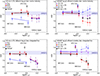 |
Fig. 3. Abundances inferred from different sulphur lines as function of logarithmic reduced equivalent width. The upper row shows results from the disc-centre intensity, and the lower row shows results from the disc-integrated flux. The left panel shows results for different sets of oscillator strengths based on the 3D non-LTE model. The right panel shows results for different models based on GRASP oscillator strengths. The black squares are the same in the left and right panels of a given row. The error bars reflect the estimated ±5% uncertainty on the measured equivalent widths. Weighted linear regressions to different line groups shown, with the S I 675 nm triplet (not present in the CIV3 set; open symbols) given zero weight in the fits. The shaded rectangle shows the solar sulphur abundance given in Asplund et al. (2021) of A(S) = 7.12 ± 0.03. |
The 3D non-LTE model gives consistent sulphur abundances from the three components of the S I 1045 nm triplet, whereas, as shown in the upper right panel of Figure 3, the other modelling approaches result in steeper trends in the inferred sulphur abundance with reduced equivalent width. Furthermore, if the 3D non-LTE model is assumed to be accurate, then the upper left panel suggests that the CIV3 data are more reliable out of the three theoretical data sets, as this set results in consistent results (on average) for the other lines together with the S I 1045 nm triplet.
Adopted oscillator strengths and recommend line-by-line and line-averaged solar sulphur abundances for different models, in the disc-centre intensity and disc-integrated flux.
On the other hand, the better overall agreement between the BSR and GRASP results may indicate that these data sets are more reliable than the CIV3 set of values. Moreover, comparisons with experimental lifetimes also suggest that the BSR and GRASP sets are slightly more reliable overall compared to CIV3 (see Li et al. 2025), although these comparisons do not include the lower or upper levels of the weak lines considered here. If these data sets are more reliable on average, then the upper right panel of Figure 3 suggests that the S I 1045 nm triplet is best modelled in 3D LTE, with 3D non-LTE in systematic error by around 0.1 dex. This would be surprising given that 3D non-LTE has consistently been demonstrated to outperform all other models, and especially 3D LTE, in various contexts (e.g. Lind & Amarsi 2024). Furthermore, the analysis we present in Section also favours 3D non-LTE over 3D LTE. Nevertheless, independent 3D non-LTE modelling of S I lines would be welcome to help verify our results.
3.3. Comparison with results from the disc-integrated flux
The spectral lines in the disc-integrated flux form in higher layers than the spectral lines in the disc-centre intensity. Consequently, the disc-integrated flux can also be analysed as a consistency check, one that is sensitive to the atmospheric stratification (3D effects) as well as for the non-LTE modelling given that departures from LTE tend to grow with height in the solar atmosphere. It should be noted, however, that uncertainties in the equivalent-width measurements, in particular placing the continuum in crowded parts of the spectrum, can render the results of this consistency test less clear.
Overall, the disc-integrated flux results in the lower left panel of Figure 3 show a similar pattern to the disc-centre intensity results in the upper left panel of that figure. Namely, with 3D non-LTE modelling, the S I 1045 nm triplet indicates a low solar sulphur abundance for all four sets of oscillator strengths. Meanwhile, the weaker lines give (on average) consistent results with the triplet when adopting the CIV3 set of oscillator strengths.
The mean result for the S I 1045 nm triplet in the disc-integrated flux is 6.99 dex, with a standard deviation of 0.03 dex, while the disc-centre intensity it is 7.05 dex with negligible scatter, based on the experimental oscillator strengths of Zerne et al. (1997). For the other lines, based on the CIV3 oscillator strengths (and excluding the S I 675 nm triplet for which there are no data in the CIV3 set) the average result in the disc-integrated flux is 6.99 dex with a standard deviation of 0.03 dex, while the disc-centre intensity it is 7.01 dex with a standard deviation of 0.04 dex.
Overall, there is good agreement between the results from the disc-centre intensity and the disc-integrated flux. However, there is a hint of a systematic bias towards lower inferred abundances in the latter case. In particular, for the S I 1045 nm triplet, the difference of 0.06 dex is somewhat larger than the line-to-line scatter. This could indicate a residual shortcoming in the 3D non-LTE models, such that the 3D non-LTE effects are slightly overestimated. Such an error would affect the synthesis of the disc-integrated flux to a greater degree than the disc-centre intensity, as the latter forms deeper in the atmosphere.
The ratio of the disc-integrated fluxes and disc-centre intensities can be used as an additional test of the S I 1045 nm triplet. This follows Amarsi et al. (2019), which considered centre-to-limb ratios for carbon lines using the centre-to-limb atlas of Stenflo (2015). Here, the observational data were drawn from the normalised Hamburg atlas (Neckel & Labs 1984) for the flux and for the intensity. The additional free parameters microturbulence and macroturbulence limit the usefulness of such a comparison for the 1D non-LTE and 1D LTE models, and so we restricted our attention to the 3D non-LTE and 3D LTE models here. The disc-integrated fluxes were broadened for stellar rotation following Dravins & Nordlund (1990) and adopting Vrot sin ι = 2.0 km s−1. Instrumental broadening was also applied to the emergent disc-centre intensities and disc-integrated fluxes, assuming R = 3.5 × 10⁵ (Neckel 1999) and adopting a sinc2 kernel. No other additional broadening was applied. The abundances were set to those inferred from the analysis of the equivalent widths in disc-centre intensity, namely 7.05 for the blue and middle components and 7.04 for the red component (Table 3).
We show the flux-to-intensity ratios in Figure 4. In comparison to observations, the 3D non-LTE model outperforms the 3D LTE model for each of the components of the S I 1045 nm triplet. It should be kept in mind that this test is carried out without the inclusion of any blending species. Still, the 3D non-LTE model shows some deviations in the wings, particularly for the strongest component for which the core also lies slightly above the observed data. As the S I 1045 nm triplet is sensitive to stellar magnetic fields (e.g. Kochukhov et al. 2024), these deviations in the wings of the ratio may be caused by the Zeeman effect, which is neglected in the present model, and thus the theoretical intensity profiles are too narrow. Interestingly, this is opposite to what is found by some other groups, where the line profiles from 3D CO5BOLD models are sometimes too broad (e.g. Deshmukh et al. 2022). The effect of some missing Zeeman broadening on the present abundance analysis is mitigated by working with equivalent widths rather than spectral line fits. Moreover, previous studies of other magnetically sensitive lines such as the O I 777 nm triplet suggest that the effects of small-scale magnetic fields in the solar atmosphere are less than 0.01 dex in abundances inferred from equivalent widths (e.g. Shchukina et al. 2016).
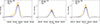 |
Fig. 4. Disc-integrated-flux-to-disc-centre-intensity ratios for the S I 1045 nm triplet. Observations from the Hamburg atlas. The thickness of the plotted lines corresponds to the ±1σ uncertainty in the 3D non-LTE and 3D LTE abundances illustrated in Figure 3, which result from a ±5% uncertainty in the measured equivalent widths. An instrumental broadening of R = 3.5 × 10⁵ is included for the synthetic intensities and fluxes, and a rotational broadening of Vrot sin ι = 2 km s−1 is included for the synthetic flux. |
Nevertheless, in future work, it may be worthwhile to explore 3D non-LTE spectrum synthesis of the S I 1045 nm triplet using 3D radiative-magnetohydrodynamics models of the solar photosphere. It may also be interesting to investigate the impact of uncertainties in the line broadening on the statistical equilibrium, although this likely corresponds to a small error overall, given that the 1D non-LTE versus 1D LTE abundance corrections for the S I 1045 nm triplet changes by less than 0.01 dex when increasing the microturbulence from 1 km s−1 to 2 km s−1.
3.4. Line-averaged solar sulphur abundance
We present line-by-line abundance results in Table 3; these are based on the disc-centre intensity and disc-integrated flux. To derive a line-averaged result, the lines were separated into two groups that suffer from different dominant systematic uncertainties, as discussed in Section . The line-averaged result was found by averaging in two groups separately.
The first group contains the three S I 1045 nm lines. These have a high sensitivity to the models (3D and non-LTE effects), but they also have precise oscillator strengths based on laboratory measurements (Zerne et al. 1997). The uncertainty in the line-averaged abundance was estimated as half the mean non-LTE effect, 3N − 3L, which was added in quadrature with half the mean 3D effect 3N − 1N. The first group gives A(S) = 7.050 ± 0.067 in the disc-centre intensity.
The second group contains the other, weaker lines. These are only moderately sensitive to the models, but a large uncertainty in their oscillator strengths is suggested by the 0.1 dex systematic shift between the CIV3 set (Deb & Hibbert 2008) compared to the GRASP set (Li et al. 2025) and the BSR set (Zatsarinny & Bartschat 2006). It is unclear which set is most reliable (Section ). To take this systematic uncertainty into account, the oscillator strengths from the CIV3 and GRASP sets were averaged together. Using the BSR set instead of the GRASP set here modifies the final result by less than 0.01 dex. As the S I 675 nm triplet is not included in the CIV3 data, and the GRASP and BSR values have a large difference of 0.07 dex that may reflect uncertainties caused by significant cancellation effects due to mixing of the 3p3(4So)5d 5Do state (Section ), this feature is deemed too questionable and is given zero weight in the line-averaged result. Nevertheless, for completeness, we list the abundances inferred from this feature in Table 3; this is based on the average of the GRASP and BSR oscillator strengths, reduced by 0.053 dex, which is half of the systematic difference between the two data sets averaged over the three weak lines. The uncertainty in the line-averaged abundance was then estimated as half of the average systematic difference (0.053 dex) added in quadrature with the standard error, which reflects the random uncertainties in the oscillator strengths and equivalent-width measurements. The second group gives A(S) = 7.068 ± 0.055 in the disc-centre intensity.
The bottom of Table 3 displays the resulting weighted mean and uncertainty after averaging the two groups using weights proportional to σ−2. The 3D non-LTE result from the disc-centre intensity is A(S) = 7.06 ± 0.04. The same weights were used to generate line-averaged results for the three other models. Repeating this exercise for the disc-integrated flux gives A(S) = 6.994 ± 0.10 for the first group and A(S) = 7.045 ± 0.054 for the second group, corresponding to a weighted mean and uncertainty of A(S) = 7.03 ± 0.05 in 3D non-LTE. It is reassuring that this result is consistent with that from the disc-centre intensity to within 1σ. This is expected because we attempted to fold in both random measurement errors and systematic modelling uncertainties.
4. Discussion
4.1. Comparison with the solar sulphur abundances of Scott et al. (2015) and Asplund et al. (2021)
The line-by-line 3D LTE results presented in Table 3 agree with those of Scott et al. (2015) to within 0.02 dex on average, after correcting for differences in the adopted oscillator strengths and including the S I 469.41 nm line. The 1D LTE results agree to within 0.01 dex on average. Some of this residual discrepancy may originate from differences between the 3D model atmosphere, the one used here being computed with the solar composition of Asplund et al. (2009), while that of Scott et al. (2015) is based on an older model computed with the metal poorer composition of Asplund et al. (2005). Some of the other differences may reflect updates in the spectrum synthesis with Scate, in particular to the atomic data and partition functions as described in Amarsi et al. (2021).
Concerning the non-LTE modelling, it is interesting to note that the 1N − 1L corrections presented in Table 2 for different lines are all within 0.02 dex of the 1N − 1L corrections in disc-centre intensity given in Scott et al. (2015) based on the model of Takeda et al. (2005). It should be noted that Scott et al. (2015) calibrated their non-LTE model so as to reduce the line-to-line scatter by scaling all of their inelastic hydrogen collisions (computed with the Drawin recipe) by a factor of 0.4. In this work, the non-LTE model takes a purely first-principles approach that includes a more physically motivated treatment of the inelastic hydrogen collisions, and therefore no calibrations were applied.
Our advocated solar sulphur abundance is different by 7.06 − 7.12 = −0.06 dex compared to that presented in Scott et al. (2015) and Asplund et al. (2021). The difference is somewhat larger than the 1σ uncertainty of ±0.04 dex arrived at here, as well as the combined 1σ uncertainty of  (even though these two uncertainties are not independent). Part of the difference is due to using a consistent 3D non-LTE approach in this work. Using an inconsistent 3D LTE + 1D non-LTE approach (3D LTE abundances with 1D non-LTE abundance corrections) as done by Scott et al. (2015) raises our result by 0.02 dex, putting it within 1σ of their result.
4.2. Comparison with the solar sulphur abundance of Caffau et al. (2007) and Caffau et al. (2011)
Another commonly-used compilation of the solar chemical composition is that of Caffau et al. (2011), which lists A(S) = 7.16 ± 0.05. The same value appears to be adopted in the compilation of Lodders et al. (2025), but with a much larger stipulated uncertainty of ±0.11 dex in their Table 2.
The result of Caffau et al. (2011) is based on the weak [S I] 1082 nm line (Caffau & Ludwig 2007), which we discuss in Section , as well as the S I 675 nm triplet, the S I 869.39 nm and 869.46 nm lines, and the S I 1045 nm triplet (Caffau et al. 2007). For the latter, they carried out a 3D LTE analysis of the disc-integrated flux. They adopted 1D non-LTE versus 1D LTE abundance corrections from Takeda et al. (2005). This model employs the Drawin recipe for the inelastic hydrogen collisions with neutral hydrogen and without any downscaling. As such, the abundance corrections for the disc-integrated flux used by Caffau et al. (2007) are less severe than the abundance corrections for the disc-centre intensity of Scott et al. (2015), which adopted a scaling of 0.4 as we discussed in Section .
Our advocated solar sulphur abundance (Section ) is different by 7.06 − 7.16 = −0.10 dex compared to that presented in Caffau et al. (2011). Adding the uncertainties of ±0.04 dex and ±0.05 dex in quadrature, the difference amounts to more than 1.5σ.
One source of the differences may be the non-LTE modelling for the S I 1045 nm triplet. Our 1D non-LTE versus 1D LTE abundance corrections for the disc-integrated flux are around 0.10 dex more negative than the values of −0.09 dex, −0.05 dex, and −0.07 dex, which Caffau et al. (2007) adopted from Takeda et al. (2005).
Another source may be the measurement of the solar spectrum. It is convenient to consider the logarithmic ratios of equivalent widths in the disc-integrated flux spectrum, dividing those given in Table 2 of Caffau et al. (2007) by those in our Table 2. For the five lines in common, these ratios are between 0.02 dex and 0.10 dex, our values being systematically smaller. Likewise, the equivalent widths given in their Table 2 tend to be larger than those given in Table 4 of Takeda et al. (2005). In fact, the equivalent widths for the disc-integrated flux reported in Caffau et al. (2007) are very close to our values for the disc-centre intensity in our Table 2. When repeating our analysis of the disc-integrated flux but adopting their equivalent widths, our 3D LTE results agree with theirs to better than 0.01 dex after averaging the lines in common. Correcting for differences in oscillator strengths slightly worsens the agreement, to 0.02 dex.
4.3. Other diagnostic S I lines of astrophysical interest
It is worth briefly discussing the [S I] 1082.1 nm line (Section ) and the S I 920 nm triplet (Section ), even though they were ultimately not folded into our advocated solar abundance. The [S I] 1082.1 nm line is sometimes used to study Galactic chemical evolution via sulphur abundances in giant stars (e.g. Ryde 2006; Jönsson et al. 2011; Matrozis et al. 2013), and the S I 920 nm triplet has been used for both giants (e.g. Lucertini et al. 2023) and dwarfs (e.g. Nissen et al. 2007), usually at lower metallicity.
4.3.1. The [S I] 1082.1 nm line
As we mentioned in Section , the [S I] 1082.1 nm line was studied in Caffau & Ludwig (2007), the results of which were folded into the recommended value of the solar sulphur abundance given in Caffau et al. (2011). They adopted log gf = −8.617 from an old version of the NIST database; this value is close to published theoretical values of −8.615 (Mendoza & Zeippen 1983) and −8.601 (Biémont & Hansen 1986). Their mean equivalent width is WI = 0.218 pm. With these values, our 3D LTE abundance is A(S) = 7.15. Our 1D abundance is only around 0.02 dex smaller, and non-LTE effects were confirmed to be negligible for this line, at least in the solar spectrum. These results are in good quantitative agreement with those reported in Table 2 of Caffau & Ludwig (2007).
However, the equivalent width of the line is difficult to precisely determine in the solar spectrum. It is strongly blended on its red side, and it sits on the outer wing of a strong feature. Our estimate is WI ≈ 0.28 pm, corresponding to a 0.11 dex larger inferred abundance. Concerning the oscillator strength, the NIST database currently states log gf = −8.73, with an accuracy rating of ‘C’ (around ±0.1 dex). This is based on the theoretical calculation of Froese Fischer et al. (2006), but corrected by around −0.03 dex for the experimental wavelength. Section 6.6 of Scott et al. (2015) states a value of log gf = −8.774 after Froese Fischer (priv. comm.). Adopting this latter value would raise the inferred abundance by a further 0.16 dex.
To shed light on this, we carried out a separate GRASP calculation for the [S I] 1082.1 nm M1 and E2 transitions. The model adopted a multi-reference set encompassing 3s23p4, 3s3p43d, 3p6, and 3s23p23d2 to produce the CSF expansion and account for the important interactions. The calculations were carried out in a layer-by-layer scheme, expanding the size of the active set of correlation orbitals up to n = 7 and l = 5 in the J = 2 symmetry block, corresponding to a maximum of 263 363 CSFs. A systematic investigation was performed on the convergence of the oscillator strength with respect to the choice of multi-reference electron-correlation effects and the size of the active set of correlation orbitals. From this analysis, we recommend a combined M1+E2 oscillator strength corresponding to log gf = −8.625.
With WI ≈ 0.28 pm and our GRASP log gf = −8.625, we arrive at A(S) = 7.27, which is difficult to reconcile with the results from the allowed S I lines, regardless of which atomic data sets are adopted for them. Despite our new oscillator strength, we arrive at the same conclusion as in Section 6.6 of Scott et al. (2015), that the weak [S I] 1082.1 nm line may be significantly blended, at least in the Sun.
4.3.2. The S I 920 nm triplet
The S I 920 nm triplet (921.29 nm, 922.81 nm, and 923.75 nm) is known to be affected by telluric water absorption when viewed using ground-based telescopes. In the IAG disc-integrated flux atlas, this renders them unusable. Fortunately, the lines appear much cleaner in the Liège disc-centre intensity atlas. The middle component has an uncertain continuum placement; from the blue and red components, we estimated equivalent widths of WI ≈ 16.44 pm and 10.80 pm, respectively. In the GRASP set, the three components have log gf = 0.395, 0.248, and 0.026 (Li et al. 2025), which is in close agreement with the BSR values via the NIST database; the lines are not present in the CIV3 set. The inferred 3D non-LTE abundance becomes A(S) ≈ 6.99, thereby also favouring a low solar sulphur abundance.
It must be stressed that the S I 920 nm triplet is saturated in the solar disc-centre intensity spectrum, with logarithmic reduced equivalent widths of −4.93 for the weakest component and −4.75 for the strongest component. They are also extremely sensitive to the models, with 3N − 3L ≈ −0.18 in the disc-centre intensity and almost 0.3 dex in the disc-integrated flux. The overall 3D non-LTE effect is slightly less severe, with 3N − 1L ≈ −0.07 in the disc-centre intensity and around −0.2 dex in the disc-integrated flux. For these reasons, this feature is considered an unreliable solar abundance diagnostic.
4.4. Comparison with the 1D non-LTE modelling of Korotin & Kiselev (2024)
The non-LTE modelling of the 1045 nm triplet plays an important role in shaping the conclusions of the current study. Thus, it is a useful consistency check to compare our model with that of an independent study. Although there are no other 3D non-LTE results in the literature, Korotin & Kiselev (2024) recently presented a detailed 1D non-LTE study of neutral and ionised sulphur in AFGK-type stars. They used ATLAS9 model atmospheres (e.g. Castelli & Kurucz 2003), the MULTI 1D non-LTE code (e.g. Carlsson 1986), and an independent approach to constructing the model atom. The complexity of the model atom in that work is similar to that used here, and key data sources that the statistical equilibrium is strongly sensitive to, including excitation by neutral hydrogen impact (Belyaev & Voronov 2020) and electron impact (Summers & O’Mullane 2011), are the same in their model as in ours. Their model does not take into account fine structure, which can have a small impact on the statistical equilibrium and thus the abundance corrections (e.g. Amarsi et al. 2024).
To make a quantitative comparison with Korotin & Kiselev (2024), 1D non-LTE calculations were carried out on the MARCS solar model atmosphere (Gustafsson et al. 2008). To better mimic their approach, ξ1D = 2.0 km s−1 was adopted. Furthermore, the equivalent widths were determined by integrating across the 1045 nm triplet as a whole, as was done in the grid of Korotin & Kiselev (2024), although the 1N − 1L values listed in Table 2 reveal that the different components may suffer rather different non-LTE effects.
The resulting 1D non-LTE versus 1D LTE abundance correction for the 1045 nm triplet in the disc-integrated flux, at an abundance of A(S) = 7.14, comes to −0.17 dex. Importantly, if repeating this same test but calculating the statistical equilibrium using a version of the reduced model atom in which all fine structure is collapsed (but still carrying out the final spectrum synthesis on the same comprehensive model atom described in Section ), the abundance correction becomes slightly less severe (−0.15 dex).
The latter result is in excellent agreement with the grid of Korotin & Kiselev (2024), which is calculated without fine structure. Interpolating their grid to the solar effective temperature and surface gravity, and adopting [Fe/H] = 0 and [S/Fe] = 0, gives a 1D non-LTE versus 1D LTE abundance correction of −0.14 dex. This is just 0.01 dex away from the result obtained here when using the reduced model atom with no fine structure, which is closer to the approach of Korotin & Kiselev (2024). This agreement makes us more confident about our non-LTE modelling and, consequently, about the overall conclusions of this study.
In lieu of full 3D non-LTE synthetic spectra or abundance corrections, the 1D non-LTE approach often gives more reliable results than 1D LTE (Lind & Amarsi 2024). Thus, we provide an extended grid of 1D non-LTE departure coefficients for sulphur levels on standard MARCS model atmospheres. These 1D non-LTE calculations employ the reduced model atom (including fine structure) and follow those presented previously in the literature for other elements (e.g. Mallinson et al. 2024; Caliskan et al. 2025) with background scattering treated as in Amarsi et al. (2022). They span the stellar parameter space described in Amarsi et al. (2020), but here with −1.5 ≤ [S/Fe] ≤ +1.5 using steps of 0.5 dex. The data are provided3 as text files and in formats that readily work with the codes SME (Piskunov & Valenti 2017) and PySME (Wehrhahn et al. 2023), with the usual caveat that the user must take care to ensure the labels of the sulphur levels in their line list match those within the grid of data.
4.5. Systematic differences between the solar photosphere and CI chondrites
Although they have long been assumed to be equal, different authors have recently pointed out the possibility of a systematic difference between the composition of CI chondrites and of the solar photosphere (e.g. Gonzalez et al. 2010; Desch et al. 2018; Jurewicz et al. 2024). All of these studies use spectroscopic results from Asplund et al. (2009) or Asplund et al. (2021), but Desch et al. (2018) added astrophysical modelling based on the compositions and ages of Solar System objects, while Jurewicz et al. (2024) included solar-wind values from the Genesis Solar Wind Sample Return (NASA Discovery 5), as well as a suite of other spectroscopic studies. The deviation between the compositions of the solar photosphere and CI chondrites are still being debated, the question being if solar spectroscopy is accurate enough to resolve such differences (e.g. Lodders et al. 2025).
In Figure 5, we plot the difference between the elemental composition of the solar photosphere and of CI chondrites (Sun − CI) as a function of 50% condensation temperature. For the photosphere, several different data sets were used, including Asplund et al. (2021) and Caffau et al. (2011), which we discuss in the context of the sulphur abundance in Sections 4.1 and 4.2, respectively, and these are based on 3D model atmospheres. A third data set is that of Magg et al. (2022), drawing on their internally derived results that are based on 1D model atmospheres constructed from a horizontally and temporally averaged 3D model. A fourth data set is that of Asplund et al. (2021), but with the sulphur abundance modified from A(S) = 7.12 ± 0.03 to A(S) = 7.06 ± 0.04, for which we advocate in Section . For the CI chondrites, the data set of Lodders (2021) is used, converted to the solar scale using A(Si) = 7.51, which is the 3D non-LTE estimate from Amarsi & Asplund (2017) adopted in Asplund et al. (2021). The reference element silicon is omitted from those data sets where it was available. Also, following Asplund et al. (2021), only elements with combined uncertainties in the photospheric and CI chondrite abundances (added in quadrature) less severe than ±0.1 dex are included.
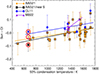 |
Fig. 5. Photospheric versus CI chondrite abundance differences as function of 50% condensation temperature from Wood et al. (2019). Photospheric data AAG21, CL11, and MB22 are from Asplund et al. (2021), Caffau et al. (2011), and Magg et al. (2022), respectively, the latter being restricted to their derivations based on a horizontally and temporally averaged 3D model. CI chondrite data are from Lodders (2021) and were converted to the solar scale with A(Si) = 7.51 from Asplund et al. (2021). Only elements with combined uncertainties less severe than ±0.1 dex are included, and the reference element silicon is omitted from those data sets where it was available. Sulphur, with Tcond = 672 K, has been circled, and the new solar sulphur abundance found in this work was used to update AAG21, forming the AAG21/new S data set. Weighted linear regressions are overplotted. |
In Figure 5, we show the weighted linear regressions for each of these data sets. By eye, all sets of photospheric data appear consistent with a linear Sun − CI versus 50% condensation temperature. According to the weighted linear regression, the gradient given by the data of Asplund et al. (2021) is 2.4σ away from a flat line, and that of Caffau et al. (2011) is 1.3σ away from a flat line. In contrast, although the line connecting them in Figure 5 is sloped, the Magg et al. (2022) data are scant and clustered around just two values of 50% condensation temperature that are only 200 K apart. So, given their moderate uncertainties, this set is consistent with having zero gradient at 1σ.
When updating the photospheric sulphur abundance in Asplund et al. (2021) to that derived in this work (AAG21/new S in Figure 5), the weighted linear regression becomes steeper. The gradient is now 2.9σ away from a flat line, compared to 2.4σ based on the unaltered Asplund et al. (2021) data set. This is because the sulphur abundance helps to drive the error-weighted trend. With Tcond = 672 K, sulphur is one of relatively few moderately volatile elements, and its abundance has relatively low uncertainty (with ±0.04 dex derived in this work). The only other elements in Figure 5 with Tcond < 800 K and combined (photospheric and CI chondrite) uncertainties less severe than ±0.1 dex are lead (Tcond = 495 K), zinc (Tcond = 704 K), and rubidium (Tcond = 752 K). In Asplund et al. (2021), these elements have more severe uncertainties than that of sulphur: ±0.08 dex, ±0.05 dex, and ±0.08 dex, respectively. Furthermore, these are all based on 3D LTE + 1D non-LTE analyses rather than consistent 3D non-LTE, and they may therefore be more susceptible to systematic errors.
The present study supports the case for systematic differences between the solar photosphere and CI chondrites that are correlated with a 50% condensation temperature. However, as discussed by Jurewicz et al. (2024), the uncertainties are large enough that different profiles may fit the Sun − CI versus 50% condensation temperature data equally well. Using a linear abundance scale (rather than logarithmic as used here), Jurewicz et al. (2024) quantified the quality of different profiles using the reduced chi-squared statistic, or mean, squared, weighted deviation, following Wendt & Carl (1991). They found that several different profiles are consistent with the Asplund et al. (2021) data, including, for example, a straight line as used here, as well as a step function with a break at around Tcond = 1350 K. When the new sulphur abundance is substituted into the set of Asplund et al. (2021), the conclusions of Jurewicz et al. (2024) do not change significantly, but the results are more consistent with the most probable value for each profile as quantified by the reduced chi-squared statistic. More precise and accurate solar-abundance measurements, particularly for other moderately volatile elements, would help with constraining different profiles and subsequently understanding the origins of the Sun − CI differences.
5. Conclusion
We reappraised the solar sulphur abundance. After considering different sets of theoretical oscillator strengths and, for the first time, consistent 3D non-LTE modelling, we argue that the abundances of A(S) = 7.12 ± 0.03 in the compilation of Asplund et al. (2021) and A(S) = 7.16 ± 0.05 in the compilation of Caffau et al. (2011) are overestimated. We advocate instead A(S) = 7.06 ± 0.04.
To confirm this argument, independent 3D non-LTE determinations would be welcome. Such efforts would clearly benefit from precise laboratory measurements of the oscillator strengths of the S I 469 nm, 675 nm, 867 nm, and 869 nm triplets. Furthermore, it would be worth repeating this study in the future using 3D non-LTE post-processing of 3D radiative-magnetohydrodynamics models of the solar photosphere to confirm the results obtained from the S I 1045 nm triplet.
The lower solar sulphur abundance supports the case for a systematic difference between the composition of the solar photosphere and of CI chondrites that is correlated with 50% condensation temperature (Gonzalez et al. 2010; Asplund et al. 2021; Jurewicz et al. 2024). This result has implications for our understanding of the early history of the Solar System, which remains under debate. To confirm the existence of this correlation and better constrain its profile, consistent 3D non-LTE abundance analyses of other moderately volatile elements would be welcome, in particular for lead, zinc, and rubidium.
A(X) ≡ log10NX/NH + 12.
Available at https://github.com/barklem/abo-cross
Acknowledgments
We thank the referee (Elisabetta Caffau) for constructive feedback that helped improve the manuscript. We also thank Sema Caliskan for valuable comments on the manuscript. AMA acknowledges support from the Swedish Research Council (VR 2020-03940) the Crafoord Foundation via the Royal Swedish Academy of Sciences (CR 2024-0015), and the European Union’s Horizon Europe research and innovation programme under grant agreement No. 101079231 (EXOHOST). WL acknowledges the support from the specialized research fund for State Key Laboratory of Solar Activity and Space Weather. AMA and WL also acknowledge support from the 2024 Chinese Academy of Sciences (CAS) President’s International Fellowship Initiative (PIFI). AJGJ acknowledges support from the NASA Laboratory Analysis of Returned Samples (LARS) Program (award number 80NSSC22K0589). This research was supported by computational resources provided by the Australian Government through the National Computational Infrastructure (NCI) under the National Computational Merit Allocation Scheme and the ANU Merit Allocation Scheme (project y89).
References
- Allen, C. W. 1973, Astrophysical Quantities, 3rd edn. (London: University of London, Athlone Press) [Google Scholar]
- Amarsi, A. M. 2015, MNRAS, 452, 1612 [NASA ADS] [CrossRef] [Google Scholar]
- Amarsi, A. M., & Asplund, M. 2017, MNRAS, 464, 264 [Google Scholar]
- Amarsi, A. M., Barklem, P. S., Asplund, M., Collet, R., & Zatsarinny, O. 2018a, A&A, 616, A89 [NASA ADS] [CrossRef] [EDP Sciences] [Google Scholar]
- Amarsi, A. M., Nordlander, T., Barklem, P. S., et al. 2018b, A&A, 615, A139 [NASA ADS] [CrossRef] [EDP Sciences] [Google Scholar]
- Amarsi, A. M., Barklem, P. S., Collet, R., Grevesse, N., & Asplund, M. 2019, A&A, 624, A111 [NASA ADS] [CrossRef] [EDP Sciences] [Google Scholar]
- Amarsi, A. M., Lind, K., Osorio, Y., et al. 2020, A&A, 642, A62 [EDP Sciences] [Google Scholar]
- Amarsi, A. M., Grevesse, N., Asplund, M., & Collet, R. 2021, A&A, 656, A113 [NASA ADS] [CrossRef] [EDP Sciences] [Google Scholar]
- Amarsi, A. M., Liljegren, S., & Nissen, P. E. 2022, A&A, 668, A68 [NASA ADS] [CrossRef] [EDP Sciences] [Google Scholar]
- Amarsi, A. M., Ogneva, D., Buldgen, G., et al. 2024, A&A, 690, A128 [NASA ADS] [CrossRef] [EDP Sciences] [Google Scholar]
- Anstee, S. D., & O’Mara, B. J. 1995, MNRAS, 276, 859 [Google Scholar]
- Asplund, M., Grevesse, N., & Sauval, A. J. 2005, ASP Conf. Ser., 336, 25 [Google Scholar]
- Asplund, M., Grevesse, N., Sauval, A. J., & Scott, P. 2009, ARA&A, 47, 481 [NASA ADS] [CrossRef] [Google Scholar]
- Asplund, M., Amarsi, A. M., & Grevesse, N. 2021, A&A, 653, A141 [NASA ADS] [CrossRef] [EDP Sciences] [Google Scholar]
- Bard, S., & Carlsson, M. 2008, ApJ, 682, 1376 [NASA ADS] [CrossRef] [Google Scholar]
- Barklem, P. S., & O’Mara, B. J. 1997, MNRAS, 290, 102 [Google Scholar]
- Barklem, P. S., O’Mara, B. J., & Ross, J. E. 1998, MNRAS, 296, 1057 [Google Scholar]
- Barklem, P. S., Belyaev, A. K., Guitou, M., et al. 2011, A&A, 530, A94 [NASA ADS] [CrossRef] [EDP Sciences] [Google Scholar]
- Belyaev, A. K., & Voronov, Y. V. 2020, ApJ, 893, 59 [NASA ADS] [CrossRef] [Google Scholar]
- Biémont, E., & Hansen, J. E. 1986, Phys. Scr., 34, 116 [Google Scholar]
- Buldgen, G., Canocchi, G., Le Saux, A., et al. 2025, Sol. Phys., 300, 97 [Google Scholar]
- Caffau, E., & Ludwig, H. G. 2007, A&A, 467, L11 [NASA ADS] [CrossRef] [EDP Sciences] [Google Scholar]
- Caffau, E., Faraggiana, R., Bonifacio, P., Ludwig, H. G., & Steffen, M. 2007, A&A, 470, 699 [NASA ADS] [CrossRef] [EDP Sciences] [Google Scholar]
- Caffau, E., Ludwig, H.-G., Steffen, M., Freytag, B., & Bonifacio, P. 2011, Sol. Phys., 268, 255 [Google Scholar]
- Caliskan, S., Amarsi, A. M., Racca, M., et al. 2025, A&A, 696, A210 [NASA ADS] [CrossRef] [EDP Sciences] [Google Scholar]
- Carlos, M., Amarsi, A. M., Nissen, P. E., & Canocchi, G. 2025, A&A, 700, A127 [NASA ADS] [CrossRef] [EDP Sciences] [Google Scholar]
- Carlsson, M. 1986, Upps. Astron. Obs. Rep., 33 [Google Scholar]
- Castelli, F., & Kurucz, R. L. 2003, in Modelling of Stellar Atmospheres, eds. N. Piskunov, W. W. Weiss, & D. F. Gray, IAU Symp., 210, A20 [Google Scholar]
- Christensen-Dalsgaard, J. 2021, Liv. Rev. Sol. Phys., 18, 2 [NASA ADS] [CrossRef] [Google Scholar]
- Civiš, S., Kramida, A., Zanozina, E. M., et al. 2024, ApJS, 274, 32 [Google Scholar]
- Collet, R., Nordlund, Ã., Asplund, M., Hayek, W., & Trampedach, R. 2018, MNRAS, 475, 3369 [NASA ADS] [CrossRef] [Google Scholar]
- Cowan, R. D. 1981, The Theory of Atomic Structure and Spectra (Berkeley, CA: University of California Press) [Google Scholar]
- Cunto, W., & Mendoza, C. 1992, Rev. Mex. Astron. Astrofis., 23 [Google Scholar]
- Deb, N. C., & Hibbert, A. 2008, At. Data Nucl. Data Tables, 94, 561 [Google Scholar]
- Delbouille, L., Roland, G., & Neven, L. 1973, Atlas photometrique du spectre solaire de [lambda] 3000 a [lambda] 10000 (Liege: Universite de Liege, Institut d’Astrophysique) [Google Scholar]
- Desch, S. J., Kalyaan, A., & O’D Alexander, C. M. 2018, ApJS, 238, 11 [NASA ADS] [CrossRef] [Google Scholar]
- Deshmukh, S. A., Ludwig, H. G., Kučinskas, A., et al. 2022, A&A, 668, A48 [NASA ADS] [CrossRef] [EDP Sciences] [Google Scholar]
- Dors, O. L., Valerdi, M., Riffel, R. A., et al. 2023, MNRAS, 521, 1969 [NASA ADS] [CrossRef] [Google Scholar]
- Dravins, D., & Nordlund, A. 1990, A&A, 228, 203 [NASA ADS] [Google Scholar]
- Froese Fischer, C., Tachiev, G., & Irimia, A. 2006, At. Data Nucl. Data Tables, 92, 607 [NASA ADS] [CrossRef] [Google Scholar]
- Froese Fischer, C., Gaigalas, G., Jönsson, P., & Bieroń, J. 2019, Comp. Phys. Commun., 237, 184 [Google Scholar]
- Gonzalez, G., Carlson, M. K., & Tobin, R. W. 2010, MNRAS, 407, 314 [NASA ADS] [CrossRef] [Google Scholar]
- Goswami, S., Vilchez, J. M., Pérez-Díaz, B., et al. 2024, A&A, 685, A81 [NASA ADS] [CrossRef] [EDP Sciences] [Google Scholar]
- Grevesse, N., & Sauval, A. J. 1998, Space Sci. Rev., 85, 161 [Google Scholar]
- Gustafsson, B., Edvardsson, B., Eriksson, K., et al. 2008, A&A, 486, 951 [NASA ADS] [CrossRef] [EDP Sciences] [Google Scholar]
- Hayek, W., Asplund, M., Collet, R., & Nordlund, Å. 2011, A&A, 529, A158 [NASA ADS] [CrossRef] [EDP Sciences] [Google Scholar]
- Hibbert, A. 1996, Phys. Scr. Vol. T, 65, 104 [Google Scholar]
- Jönsson, H., Ryde, N., Nissen, P. E., et al. 2011, A&A, 530, A144 [NASA ADS] [CrossRef] [EDP Sciences] [Google Scholar]
- Jönsson, P., Gaigalas, G., Fischer, C. F., et al. 2023, Atoms, 11, 68 [CrossRef] [Google Scholar]
- Jurewicz, A. J. G., Amarsi, A. M., Burnett, D. S., & Grevesse, N. 2024, Meteorit. Planet. Sci., 59, 3193 [Google Scholar]
- Kama, M., Shorttle, O., Jermyn, A. S., et al. 2019, ApJ, 885, 114 [Google Scholar]
- Kaulakys, B. P. 1985, J. Phys. B: At. Mol. Opt. Phys., 18, L167 [Google Scholar]
- Kaulakys, B. P. 1986, JETP, 91, 391 [Google Scholar]
- Kaulakys, B. P. 1991, J. Phys. B: At. Mol. Opt. Phys., 24, L127 [NASA ADS] [CrossRef] [Google Scholar]
- Keyte, L., Kama, M., Chuang, K.-J., et al. 2024, MNRAS, 528, 388 [NASA ADS] [CrossRef] [Google Scholar]
- Kochukhov, O., Amarsi, A. M., Lavail, A., et al. 2024, A&A, 689, A36 [NASA ADS] [CrossRef] [EDP Sciences] [Google Scholar]
- Korotin, S. A., & Kiselev, K. O. 2024, Astron. Rep., 68, 1159 [Google Scholar]
- Kramida, A. 2024, Eur. Phys. J. D, 78, 36 [Google Scholar]
- Kurucz, R. L. 1995, ASP Conf. Ser., 78, 205 [NASA ADS] [Google Scholar]
- Laming, J. M., Vourlidas, A., Korendyke, C., et al. 2019, ApJ, 879, 124 [Google Scholar]
- Leenaarts, J., & Carlsson, M. 2009, ASP Conf. Ser., 415, 87 [Google Scholar]
- Li, W., Amarsi, A. M., Papoulia, A., Ekman, J., & Jönsson, P. 2021, MNRAS, 502, 3780 [NASA ADS] [CrossRef] [Google Scholar]
- Li, M. C., Li, W., Jönsson, P., Amarsi, A. M., & Grumer, J. 2023a, ApJS, 265, 26 [NASA ADS] [CrossRef] [Google Scholar]
- Li, W., Jönsson, P., Amarsi, A. M., Li, M. C., & Grumer, J. 2023b, A&A, 674, A54 [NASA ADS] [CrossRef] [EDP Sciences] [Google Scholar]
- Li, Y., Gaigalas, G., Li, W., Chen, C., & Jönsson, P. 2023c, Atoms, 11, 70 [Google Scholar]
- Li, W., Amarsi, A. M., & Jönsson, P. 2025, A&A, submitted [Google Scholar]
- Lind, K., & Amarsi, A. M. 2024, ARA&A, 62, 475 [NASA ADS] [CrossRef] [Google Scholar]
- Lodders, K. 2021, Space Sci. Rev., 217, 44 [NASA ADS] [CrossRef] [Google Scholar]
- Lodders, K., Bergemann, M., & Palme, H. 2025, Space Sci. Rev., 221, 23 [Google Scholar]
- Lucertini, F., Monaco, L., Caffau, E., Bonifacio, P., & Mucciarelli, A. 2022, A&A, 657, A29 [NASA ADS] [CrossRef] [EDP Sciences] [Google Scholar]
- Lucertini, F., Monaco, L., Caffau, E., et al. 2023, A&A, 671, A137 [NASA ADS] [CrossRef] [EDP Sciences] [Google Scholar]
- Magg, E., Bergemann, M., Serenelli, A., et al. 2022, A&A, 661, A140 [NASA ADS] [CrossRef] [EDP Sciences] [Google Scholar]
- Magic, Z., Collet, R., Asplund, M., et al. 2013, A&A, 557, A26 [NASA ADS] [CrossRef] [EDP Sciences] [Google Scholar]
- Mallinson, J. W. E., Lind, K., Amarsi, A. M., & Youakim, K. 2024, A&A, 687, A5 [NASA ADS] [CrossRef] [EDP Sciences] [Google Scholar]
- Martin, W. C., Zalubas, R., & Musgrove, A. 1990, J. Phys. Chem. Ref. Data, 19, 821 [NASA ADS] [CrossRef] [Google Scholar]
- Matrozis, E., Ryde, N., & Dupree, A. K. 2013, A&A, 559, A115 [NASA ADS] [CrossRef] [EDP Sciences] [Google Scholar]
- Mendoza, C., & Zeippen, C. J. 1983, MNRAS, 202, 981 [NASA ADS] [CrossRef] [Google Scholar]
- Mohorian, M., Kamath, D., Menon, M., et al. 2025a, MNRAS, 538, 1339 [Google Scholar]
- Mohorian, M., Kamath, D., Menon, M., et al. 2025b, PASA, submitted [arXiv:2510.16691] [Google Scholar]
- Neckel, H. 1999, Sol. Phys., 184, 421 [Google Scholar]
- Neckel, H., & Labs, D. 1984, Sol. Phys., 90, 205 [Google Scholar]
- Nissen, P. E., Akerman, C., Asplund, M., et al. 2007, A&A, 469, 319 [NASA ADS] [CrossRef] [EDP Sciences] [Google Scholar]
- Nordlund, Å., Stein, R. F., & Asplund, M. 2009, Liv. Rev. Sol. Phys., 6, 2 [Google Scholar]
- Perdigon, J., de Laverny, P., Recio-Blanco, A., et al. 2021, A&A, 647, A162 [NASA ADS] [CrossRef] [EDP Sciences] [Google Scholar]
- Pérez-Montero, E., Pérez-Díaz, B., Vílchez, J. M., et al. 2025, Open J. Astrophys., submitted [arXiv:2506.14736] [Google Scholar]
- Piskunov, N., & Valenti, J. A. 2017, A&A, 597, A16 [NASA ADS] [CrossRef] [EDP Sciences] [Google Scholar]
- Podobedova, L. I., Kelleher, D. E., & Wiese, W. L. 2009, J. Phys. Chem. Ref. Data, 38, 171 [NASA ADS] [CrossRef] [Google Scholar]
- Ralchenko, Y., & Kramida, A. 2020, Atoms, 8, 56 [NASA ADS] [CrossRef] [Google Scholar]
- Reiners, A., Mrotzek, N., Lemke, U., Hinrichs, J., & Reinsch, K. 2016, A&A, 587, A65 [NASA ADS] [CrossRef] [EDP Sciences] [Google Scholar]
- Rodríguez Díaz, L. F., Lagae, C., Amarsi, A. M., et al. 2024, A&A, 688, A212 [NASA ADS] [CrossRef] [EDP Sciences] [Google Scholar]
- Ryde, N. 2006, A&A, 455, L13 [NASA ADS] [CrossRef] [EDP Sciences] [Google Scholar]
- Scott, P., Grevesse, N., Asplund, M., et al. 2015, A&A, 573, A25 [NASA ADS] [CrossRef] [EDP Sciences] [Google Scholar]
- Seaton, M. J. 1962, Proc. Phys. Soc., 79, 1105 [NASA ADS] [CrossRef] [Google Scholar]
- Seaton, M. J. 1995, The Opacity Project (Institute of Physics Pub.) [Google Scholar]
- Shchukina, N., Sukhorukov, A., & Trujillo Bueno, J. 2016, A&A, 586, A145 [NASA ADS] [CrossRef] [EDP Sciences] [Google Scholar]
- Stein, R. F., Nordlund, Å., Collet, R., & Trampedach, R. 2024, ApJ, 970, 24 [NASA ADS] [CrossRef] [Google Scholar]
- Stenflo, J. O. 2015, A&A, 573, A74 [NASA ADS] [CrossRef] [EDP Sciences] [Google Scholar]
- Summers, H. P., & O’Mullane, M. G. 2011, AIP Conf. Ser., 1344, 179 [NASA ADS] [Google Scholar]
- Takeda, Y. 2022, Sol. Phys., 297, 4 [NASA ADS] [CrossRef] [Google Scholar]
- Takeda, Y., Hashimoto, O., Taguchi, H., et al. 2005, PASJ, 57, 751 [NASA ADS] [Google Scholar]
- van Regemorter, H. 1962, ApJ, 136, 906 [NASA ADS] [CrossRef] [Google Scholar]
- Wehrhahn, A., Piskunov, N., & Ryabchikova, T. 2023, A&A, 671, A171 [NASA ADS] [CrossRef] [EDP Sciences] [Google Scholar]
- Wendt, I., & Carl, C. 1991, Chem. Geol. Isot. Geos., 86, 275 [Google Scholar]
- Wood, B. J., Smythe, D. J., & Harrison, T. 2019, Am. Mineral., 104, 844 [NASA ADS] [CrossRef] [Google Scholar]
- Zatsarinny, O., & Bartschat, K. 2006, J. Phys. B At. Mol. Opt. Phys., 39, 2861 [Google Scholar]
- Zerne, R., Caiyan, L., Berzinsh, U., & Svanberg, S. 1997, Phys. Scr., 56, 459 [NASA ADS] [CrossRef] [Google Scholar]
- Zhou, Y., Amarsi, A. M., Aguirre Børsen-Koch, V., et al. 2023, A&A, 677, A98 [NASA ADS] [CrossRef] [EDP Sciences] [Google Scholar]
All Tables
Adopted oscillator strengths and recommend line-by-line and line-averaged solar sulphur abundances for different models, in the disc-centre intensity and disc-integrated flux.
All Figures
|
Fig. 1. Gas-temperature distribution with vertical logarithmic optical depth in the 3D model atmosphere (blue). The T − log τ relation of the corresponding 1D model atmosphere is also shown (orange). The full widths at half maximum of the line-profile’s integrated, 1D, non-LTE contribution functions to the line depressions (Amarsi 2015) are shown for the diagnostic S I lines (the line-averaged result is shown for the S I 1045 nm triplet). These are presented for both the disc-centre intensity (black) and disc-integrated flux (red) with circles indicating the positions of the peaks. |
| In the text | |
|
Fig. 2. Grotrian diagram for comprehensive (left) and reduced (right) model atoms used in this work. Terms for which fine-structure are unresolved are shown as short blue horizontal lines. Super levels in the reduced model atom are shown as long, blue horizontal lines. Transitions are shown as slanted grey lines; those used as abundance diagnostics are shown as coloured slanted lines in the right panel and labelled in the legend. |
| In the text | |
|
Fig. 3. Abundances inferred from different sulphur lines as function of logarithmic reduced equivalent width. The upper row shows results from the disc-centre intensity, and the lower row shows results from the disc-integrated flux. The left panel shows results for different sets of oscillator strengths based on the 3D non-LTE model. The right panel shows results for different models based on GRASP oscillator strengths. The black squares are the same in the left and right panels of a given row. The error bars reflect the estimated ±5% uncertainty on the measured equivalent widths. Weighted linear regressions to different line groups shown, with the S I 675 nm triplet (not present in the CIV3 set; open symbols) given zero weight in the fits. The shaded rectangle shows the solar sulphur abundance given in Asplund et al. (2021) of A(S) = 7.12 ± 0.03. |
| In the text | |
|
Fig. 4. Disc-integrated-flux-to-disc-centre-intensity ratios for the S I 1045 nm triplet. Observations from the Hamburg atlas. The thickness of the plotted lines corresponds to the ±1σ uncertainty in the 3D non-LTE and 3D LTE abundances illustrated in Figure 3, which result from a ±5% uncertainty in the measured equivalent widths. An instrumental broadening of R = 3.5 × 10⁵ is included for the synthetic intensities and fluxes, and a rotational broadening of Vrot sin ι = 2 km s−1 is included for the synthetic flux. |
| In the text | |
|
Fig. 5. Photospheric versus CI chondrite abundance differences as function of 50% condensation temperature from Wood et al. (2019). Photospheric data AAG21, CL11, and MB22 are from Asplund et al. (2021), Caffau et al. (2011), and Magg et al. (2022), respectively, the latter being restricted to their derivations based on a horizontally and temporally averaged 3D model. CI chondrite data are from Lodders (2021) and were converted to the solar scale with A(Si) = 7.51 from Asplund et al. (2021). Only elements with combined uncertainties less severe than ±0.1 dex are included, and the reference element silicon is omitted from those data sets where it was available. Sulphur, with Tcond = 672 K, has been circled, and the new solar sulphur abundance found in this work was used to update AAG21, forming the AAG21/new S data set. Weighted linear regressions are overplotted. |
| In the text | |
Current usage metrics show cumulative count of Article Views (full-text article views including HTML views, PDF and ePub downloads, according to the available data) and Abstracts Views on Vision4Press platform.
Data correspond to usage on the plateform after 2015. The current usage metrics is available 48-96 hours after online publication and is updated daily on week days.
Initial download of the metrics may take a while.