| Issue |
A&A
Volume 703, November 2025
|
|
|---|---|---|
| Article Number | L4 | |
| Number of page(s) | 5 | |
| Section | Letters to the Editor | |
| DOI | https://doi.org/10.1051/0004-6361/202557165 | |
| Published online | 31 October 2025 | |
Letter to the Editor
Quasi-periodic oscillations in optical color evolutions to support sub-parsec binary black hole systems in broad line active galactic nuclei
Guangxi Key Laboratory for Relativistic Astrophysics, School of Physical Science and Technology, GuangXi University, No. 100, Daxue Road, Nanning 530004, PR China
⋆ Corresponding author: This email address is being protected from spambots. You need JavaScript enabled to view it.
Received:
9
September
2025
Accepted:
15
October
2025
Abstract
Optical quasi-periodic oscillations (QPOs) with periodicities that range from hundreds to thousands of days have been accepted as an efficient indicator for sub-parsec (sub-pc) binary black hole systems (BBHs) in broad line active galactic nuclei (BLAGN). However, considering the intrinsic variability (red noise) of BLAGN, it is still an open question on the physical origin of detected optical QPOs from AGN variability or truly from sub-pc BBHs. Here, a simple method is proposed to support optical QPOs related to sub-pc BBHs by detecting QPOs in time-dependent optical color evolutions of BLAGN. Periodic variations of obscurations are expected on optical light curves related to sub-pc BBHs, but there should be non-periodic variable obscurations on optical light curves in normal BLAGN. Through simulated optical light curves for intrinsic AGN variability by continuous autoregressive processes with time durations of around 2800 days (similar to the time durations of light curves in the ZTF), the probability is definitely lower than 3.3 × 10⁻⁷ that QPOs can be detected in the corresponding optical color evolutions, but about 3.1 × 10⁻² that optical QPOs with periodicity shorter than 1400 days (at least two cycles) can be detected in the simulated single-band light curves. Therefore, the confidence level is definitely higher than 5σ to support the QPOs in color evolutions not related to intrinsic AGN variability, but truly related to sub-pc BBHs. In the near future, the proposed method can be applied to searching for reliable optical QPOs in BLAGN through multi-band light curves from the ZTF and the upcoming LSST.
Key words: galaxies: active / galaxies: nuclei / galaxies: photometry / quasars: supermassive black holes
© The Authors 2025
 Open Access article, published by EDP Sciences, under the terms of the Creative Commons Attribution License (https://creativecommons.org/licenses/by/4.0), which permits unrestricted use, distribution, and reproduction in any medium, provided the original work is properly cited.
This article is published in open access under the Subscribe to Open model. This email address is being protected from spambots. You need JavaScript enabled to view it. to support open access publication.
1. Introduction
Sub-parsec (sub-pc) binary black hole systems (BBHs) have been commonly expected as natural products of galaxy mergers and evolution (Begelman et al. 1980; Silk & Rees 1998; Merritt 2006; Satyapal et al. 2014; Mannerkoski et al. 2022; Attard et al. 2024; Casey-Clyde et al. 2025). Considering the periodic orbital rotations of two BH accreting systems in sub-pc BBHs, long-standing optical quasi-periodic oscillations (QPOs) related to periodic obscurations have been widely accepted as the efficient indicator for sub-pc BBHs. To date, through optical QPOs with periodicities from hundreds to thousands of days, around 300 sub-pc BBHs have been reported in broad line active galactic nuclei (BLAGN) (e.g., the samples of candidates in Graham et al. 2015a; Charisi et al. 2016; Foustoul et al. 2025 and the individual candidates in Graham et al. 2015b; Liu et al. 2015; Kovacevic et al. 2019, 2020; Zheng et al. 2016; Serafinelli et al. 2020; Liao et al. 2021, 2025; Zhang 2022a,b, 2023a,b, 2025; Adhikari et al. 2024).
Although more and more long-standing optical QPOs have been reported in BLAGN, whether the detected QPOs were intrinsically related to sub-pc BBHs is also an open question. More specifically, red noise, traced by intrinsic AGN variability as one of fundamental characteristics of AGN (Wagner & Witzel 1995; Ulrich et al. 1997; Baldassare et al. 2018; Benati-Goncalves et al. 2025), can lead to mathematically determined fake optical QPOs. The effects of red noise on optical QPOs were first shown in Vaughan et al. (2016). Then, in our recent works in Zhang (2023a,b, 2025), Liao et al. (2025), such effects of red noise have been discussed, especially on corresponding confidence levels to support the detected optical QPOs not related to intrinsic AGN variability through mathematical simulations.
Due to the apparent and inevitable effects of red noise on optical QPOs in BLAGN, it is a challenge to propose a method applied to improve the confidence levels for detected optical QPOs in BLAGN, which is our main objective. Here, not through a single-band optical light curve but through optical color evolutions between two-band optical light curves, an improved method is proposed to support sub-pc BBHs with confidence levels higher than 5σ in this manuscript through simulated results.
For a single-band optical light curve in BLAGN, as discussed in Kelly et al. (2009), Kozlowski et al. (2010), MacLeod et al. (2010), Ma et al. (2024), it can be mathematically described by the widely accepted damped random walk (DRW) process or the first-order continuous autoregressive (CAR) process with two basic process parameters of the intrinsic variability timescale τ and intrinsic variability amplitude σ*. Certainly, improved higher-order continuous-time autoregressive moving average (CARMA) models have been proposed in Kelly et al. (2014), Yu et al. (2022), Kishore et al. (2024) to describe AGN variability with more subtle features. However, due to a greater number of free model parameters that are difficult to constrain, the CARMA models are not convenient models for our mathematical simulations.
Based on single-band optical light curves created by DRW and CAR processes in BLAGN, the other optical band light curve can be simply simulated after considering time lags and probably different emission structures of two-band optical emissions. Time lags of several days between two-band optical light curves have been discussed for more than three decades (see Edelson et al. 1996, 2015; Sergeev et al. 2005; Yu et al. 2020; Kammoun et al. 2021; Netzer 2022; Wang et al. 2025). Furthermore, considering the same source of ionization variability, similar variability patterns are accepted for optical light curves in different optical bands, but convolved with a kernel function for considerations of probably different structure information, as was done in Zu et al. (2016) and Ma et al. (2024).
In this manuscript, considering no variable obscurations on intrinsic AGN variability but apparent time lags between two-band optical light curves, an improved method through detecting QPOs in optical color (difference between two-band optical light curves) evolutions is mainly discussed to support sub-pc BBHs with higher confidence levels. The manuscript is organized as follows. Section 2 presents the main hypotheses and results. Our main conclusions are given in Section 3. Throughout the manuscript, we have adopted the cosmological parameters of H0 = 70 km s−1 Mpc−1, Ωm = 0.3, and ΩΛ = 0.7.
2. Hypotheses, results, and discussions
2.1. Main results through the simulated light curves
As described in the Introduction, the variability of optical color evolutions from two-band light curves are mainly considered. Therefore, among the current public sky survey projects, the Zwicky Transient Facility (ZTF) (Bellm et al. 2019; Dekany et al. 2020) is the most suitable choice at the current stage, which provides optical g- and r-band light curves with time durations of around 2800 days.
Before creating artificial optical two-band light curves of BLAGN, the mean values of two-band apparent magnitudes can be simply determined by the correlation between Sloan Digital Sky Survey (SDSS) g-band and r-band magnitudes (mg, mr) of 3530 low-redshift (z < 0.35) quasars listed in Shen et al. (2011). As shown in Fig. 1, there is a strong linear correlation with the Spearman rank correlation coefficient 0.96 (Pnull < 10−10). Considering uncertainties in both coordinates, through the least trimmed squares regression technique (Cappellari et al. 2013), the correlation can be described as
 (1)
(1)
with RMS scatter of about 0.154. Although the apparent magnitudes are collected from SDSS not from ZTF, there are few effects on our following results. Then, the equation can be applied to determine the apparent magnitudes of the following artificial optical two-band light curves by the following two steps.
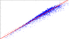 |
Fig. 1. Correlation between SDSS g- and r-band apparent magnitudes of 3530 low-redshift quasars. The solid and dashed red lines show the best fitting results and corresponding 5σ confidence bands. |
First, through the CAR process (Kelly et al. 2009), a single-band optical light curve LC1, 0(t) can be created as
 (2)
(2)
with ϵ(t) as a white noise process with zero mean and variance equal to 1. The corresponding time duration of t is about 2800 days and the time step is about 3 days, similar to the time durations and time steps of high-quality light curves in ZTF. Here the time t is created by 993 random values from 0 to 2800 (corresponding IDL code, t=randomu(seed, 993) * 2800) & t=t(sort(t)) & t=t(rem_dup(t)). The CAR process parameters are randomly collected from 100 days to 1500 days for τ and from 0.003 mag/day0.5 to 0.04 mag/day0.5 for σ*, which are common values for BLAGN as shown in Kelly et al. (2009), Kozlowski et al. (2010), MacLeod et al. (2010). Then, the mean apparent magnitudes m1 (assumed in g-band) are randomly collected from 16 mags to 20 mags, as shown in Fig. 1.
Second, light curves LC2(t) from the other optical band can be created as follows. Considering the results in Fig. 1, the mean apparent magnitude m2 (assumed in r-band) is collected by
 (3)
(3)
with k1 and k2 as random values determined by normal distributions centered at zero and with second moments to be the corresponding uncertainties of 0.057 and 0.003 determined in Equation (1). Considering a time lag Δt between g-band and r-band with random values from 0 days to 5 days (the value large enough) as more recent discussions in Netzer (2022), Wang et al. (2025), the delayed light curve can be described as
 (4)
(4)
Then, considering different structure information of emission regions for the two-band optical light curves, a Gaussian convolution function G(σt) with second moment σt randomly from 0 days to 5 days is applied as
![Mathematical equation: $$ \begin{aligned} k&\in [0, 1],\nonumber \\ LC_1(t)&=LC_{1,0}(t)\ \ \ \ \ \ (k<0.5),\nonumber \\ LC_2(t)&= LC_{2,0}(t) \otimes G(\sigma _t) \ \ \ \ \ \ (k < 0.5),\nonumber \\ LC_2(t)&= LC_{2,0}(t)\ \ \ \ \ \ (k\ge 0.5),\nonumber \\ LC_1(t)&= LC_{1,0}(t) \otimes G(\sigma _t) \ \ \ \ \ \ (k\ge 0.5), \end{aligned} $$](/articles/aa/full_html/2025/11/aa57165-25/aa57165-25-eq5.gif) (5)
(5)
with k as a random value from 0 to 1. Then, the color evolution
 (6)
(6)
can be calculated.
Based on simulated LC1(t) and CL(t), it is interesting to check whether probable fake QPOs can be detected in the artificial light curves tightly related to AGN variability (red noise). To repeat the two steps above three million times, QPOs can be checked through the LC1(t) and CL(t), which will provide clues to determine probability for detecting fake QPOs in the corresponding light curves. Here, the commonly accepted Lomb-Scargle (LS) periodogram (VanderPlas 2018) has been accepted to detect QPOs. Figure 2 shows examples of LC1, 0(t) and LC2, 0(t), LC1(t) and LC2(t), and CL(t) and the corresponding LS powers. As the shown examples, it is clear that the CAR created artificial light curves can lead to detected fake QPOs with a significance level higher than 5σ in single-band light curves. However, such fake QPOs cannot be detected in the corresponding CL(t), providing clues that probability of detecting fake QPOs in CL(t) should be significantly smaller than in single-band optical light curves.
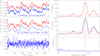 |
Fig. 2. Left panels: Light curves of LC1, 0(t) (in blue) and LC2, 0(t) (in red) (top left panel); LC1(t) (in blue) and LC2(t) (in red) (middle left panel); and Color(t) (bottom left panel). Right panels: Corresponding LS powers. In the top right panel (middle right panel), the solid line in blue and red show the results through LC1, 0(t) (LC1(t)) and LC2, 0(t) (LC2(t)), respectively. In each right panel, the horizontal dashed red line marks the 5σ significance level (determined by the input false alarm probability to be 3 × 10⁻⁷); the vertical dashed red line marks the position of periodicity around 812 days determined in LC1(t). |
Among the three million (Nt = 3d6) simulated cases, two probabilities of detecting fake QPOs are determined. The first probability P1 is for detecting QPOs in LC1(t) with a significance level higher than 5σ and the corresponding periodicity TP1 smaller than 1400 days (to support the artificial LC1(t) including at least two cycles), leading to N1 = 94527 LC1(t) to be collected. Therefore, through intrinsic AGN variability, fake optical QPOs can be detected, and the corresponding probability P1 is about N1/Nt ∼ 3.1 × 10⁻². Meanwhile, the probability P12 ∼ 3.1% can also be determined for detecting QPOs in LC2(t) after considering the same criteria applied for P1, due to N2 = 94579 LC2(t) to be collected. There are the same probabilities for detecting fake QPOs in the simulated LC1(t) and LC2(t). Furthermore, for the 94527 LC1(t) including fake QPOs, Fig. A.1 in the Appendix shows distributions of the parameters of τ, σ, Δt, and σt applied in the procedure above, indicating that smaller τ should favor the detection of fake QPOs in the simulated light curves. Moreover, in Zhang (2025) for optical QPOs in PG 1411, the probability is P0 ∼ 4.8 × 10⁻⁴, much smaller than P1, for detecting fake QPOs through the CAR process simulated light curves. However, in Zhang (2025), additional criteria have been applied: periodicity from 450 days to 650 days and sine function described simulated light curves. If the two additional criteria are accepted, the number should be N1 ∼ 2193, leading to the probability P10 ∼ 7.3 × 10⁻⁴ similar to P0. The small difference between P10 and P0 is probably due to different qualities of simulated light curves, different time steps, and different time durations.
The second probability P2 is for detecting QPOs in CL(t) with a significance level higher than 5σ and also with the corresponding periodicity TP2 similar to the TP1 detected in LC1(t), leading to not one CL(t) being collected. Here, we simply accepted the similar periodicities in LC1(t) and in CL(t), if  is between 0.85 and 1.15. Therefore, through the AGN variability expected color evolution CL(t), no fake QPOs can be detected, and the corresponding probability is approximately P2 < 1/Nt ∼ 3.3 × 10⁻⁷, about 9.5 × 10⁴ times smaller than P1. Based on the determined P2, we can safely state that once QPOs are detected in CL(t), the confidence level should be higher than 5σ to support that the detected QPOs are not related to intrinsic AGN variability. Therefore, detecting QPOs in CL(t) should provide stable evidence to support QPOs not related to intrinsic AGN variability, but truly related to sub-pc BBHs.
2.2. Application in the SDSS J1609+1756
The discussed results above are based on the given time information of light curves and randomly collected process parameters. It is necessary to test such results in long-term optical two-band light curves of a real BLAGN. Then, we checked the reported optical QPOs with periodicities of about 340 days in the blue quasar SDSS J1609+1756 in Zhang (2023a) through long-term ZTF light curves. The g- and r-band light curves of LCg(t) and LCr(t) and the CL(t) = LCg(t)−LCr(t) are shown in top two panels of Fig. 3. The corresponding LS powers of CL(t) are shown in the bottom panel of Fig. 3, leading to a periodicity of about 320 days in CL(t). Then, based on the time information t of the g-band light curve and the determined τ ∼ 140 days and σ* ∼ 0.035mag/day0.5 reported in Zhang (2023a), three million simulations were performed as what have recently done above, three million simulations were performed reproducing the above-described scenario, still leading to no case collected with apparent QPOs in CL(t). Therefore, relative to the probability of about 0.26% in Zhang (2023a) for detecting fake QPOs in CAR procedure simulated single-band optical light curves, the probability of detecting QPOs in CL(t) is clearly lower than 3.3 × 10⁻⁷ (< 1/3d6). In other words, the confidence level is higher than 5σ for the optical QPOs in the blue quasar SDSS J1609+1756.
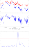 |
Fig. 3. Top panel: ZTF g-band (blue symbols) and r-band (red symbols) light curves of SDSS J1609+1756. Middle panel: CL(t). Bottom panel: Determined LS powers of CL(t). The horizontal dashed red line is the 5σ significance level. |
3. Conclusions
Considering the periodic variations in obscurations on light curves related to sub-pc BBHs, but no variable obscurations on light curves of normal BLAGN, we proposed a method to support detected QPOs not related to red noise (AGN intrinsic variability), but truly related to sub-pc BBHs, through reliable periodic features in time-dependent optical color evolutions. Among 3 × 10⁶ simulated cases of CL(t) by artificial two-band optical light curves for intrinsic AGN variability by the CAR process, the probability for detecting QPOs in CL(t) is definitely lower than 3.3 × 10⁻⁷, which is about 9.5 × 10⁴ times lower than the probability for detecting QPOs in single-band light curves. Therefore, a confidence level higher than 5σ can be safely accepted for optical QPOs in a BLAGN if there are QPOs in the corresponding optical color evolutions. The method was applied in the blue quasar SDSS J1609+1756 to support the reported optical QPOs related to sub-pc BBHs. The method proposed in this manuscript can be efficiently applied for searching for reliable optical QPOs in BLAGN through multi-band light curves from the ZTF and the upcoming project of Legacy Survey of Space and Time (LSST) in the near future.
Acknowledgments
Zhang gratefully acknowledge the anonymous referee for giving us constructive comments and suggestions to greatly improve the paper. Zhang gratefully thanks the kind financial support from GuangXi University and the kind grant support from NSFC-12173020, 12373014 and from the Guangxi Talent Programme (Highland of Innovation Talents). This article is kindly dedicated to celebrating the 60th birthday of my most respected supervisor, Prof. Wang TingGui. This manuscript has made use of the data from ZTF (https://www.ztf.caltech.edu), and use of the IDL code of lts_linefit.pro (https://users.physics.ox.ac.uk/~cappellari/) and scargle.pro (http://astro.uni-tuebingen.de/software/idl/aitlib/timing/scargle.html).
References
- Adhikari, S., Penil, P., Westernacher-Schneider, J. R., et al. 2024, ApJ, 965, 124 [CrossRef] [Google Scholar]
- Attard, K., Gualandris, A., Read, J. I., & Dehnen, W. 2024, MNRAS, 529, 2150 [Google Scholar]
- Baldassare, V. F., Geha, M., & Greene, J. 2018, ApJ, 868, 152 [NASA ADS] [CrossRef] [Google Scholar]
- Begelman, M. C., Blandford, R. D., & Rees, M. J. 1980, Nature, 287, 307 [Google Scholar]
- Bellm, E. C., Kulkarni, S. R., Barlow, T., et al. 2019, PASP, 131, 068003 [Google Scholar]
- Benati-Goncalves, H., Panda, S., Storchi-Bergmann, T., Cackett, E. M., & Eracleous, M. 2025, ApJ, 988, 27 [Google Scholar]
- Cappellari, M., Scott, N., Alatalo, K., et al. 2013, MNRAS, 432, 1709 [Google Scholar]
- Casey-Clyde, J. A., Mingarelli, C. M. F., Greene, J. E., et al. 2025, ApJ, 987, 106 [Google Scholar]
- Charisi, M., Bartos, I., Haiman, Z., et al. 2016, MNRAS, 463, 2145 [Google Scholar]
- Dekany, R., Smith, R. M., Riddle, R., et al. 2020, PASP, 132, 038001 [NASA ADS] [CrossRef] [Google Scholar]
- Edelson, R. A., Alexander, T., Crenshaw, D. M., et al. 1996, ApJ, 470, 364 [NASA ADS] [CrossRef] [Google Scholar]
- Edelson, R., Gelbord, J. M., Horne, K., et al. 2015, ApJ, 806, 129 [NASA ADS] [CrossRef] [Google Scholar]
- Foustoul, V., Webb, N. A., Mignon-Risse, R., et al. 2025, A&A, 699, A55 [NASA ADS] [CrossRef] [EDP Sciences] [Google Scholar]
- Graham, M. J., Djorgovski, S. G., Stern, D., et al. 2015a, MNRAS, 453, 1562 [Google Scholar]
- Graham, M. J., Djorgovski, S. G., Stern, D., et al. 2015b, Nature, 518, 74 [Google Scholar]
- Kammoun, E. S., Papadakis, I. E., & Dovciak, M. 2021, MNRAS, 503, 4163 [CrossRef] [Google Scholar]
- Kelly, B. C., Bechtold, J., & Siemiginowska, A. 2009, ApJ, 698, 895 [Google Scholar]
- Kelly, B. C., Becker, A. C., Sobolewska, M., Siemiginowska, A., & Uttley, P. 2014, ApJ, 788, 33 [NASA ADS] [CrossRef] [Google Scholar]
- Kishore, S., Gupta, A. C., & Wiita, P. G. 2024, ApJ, 960, 11 [NASA ADS] [CrossRef] [Google Scholar]
- Kovacevic, A. B., Popovic, L. C., Simic, S., & Ilic, D. 2019, ApJ, 871, 32 [Google Scholar]
- Kovacevic, A. B., Yi, T., Dai, X., et al. 2020, MNRAS, 494, 4069 [CrossRef] [Google Scholar]
- Kozlowski, S., Kochanek, C. S., Udalski, A., et al. 2010, ApJ, 708, 927 [CrossRef] [Google Scholar]
- Liao, W., Chen, Y., Liu, X., et al. 2021, MNRAS, 500, 4025 [NASA ADS] [Google Scholar]
- Liao, G. L., Chen, X. Q., Zheng, Q., Liu, Y. L., & Zhang, X. G. 2025, A&A, 698, A265 [NASA ADS] [CrossRef] [EDP Sciences] [Google Scholar]
- Liu, T., Gezari, S., Heinis, S., et al. 2015, ApJ, 803, L16 [NASA ADS] [CrossRef] [Google Scholar]
- Ma, Q., Wen, Y., Wu, X., Gu, H., & Fu, Y. 2024, ApJ, 966, 5 [Google Scholar]
- MacLeod, C. L., Ivezic, Z., Kochanek, C. S., et al. 2010, ApJ, 721, 1014 [Google Scholar]
- Mannerkoski, M., Johansson, P. H., Rantala, A., et al. 2022, ApJ, 929, 167 [NASA ADS] [CrossRef] [Google Scholar]
- Merritt, D. 2006, ApJ, 648, 976 [NASA ADS] [CrossRef] [Google Scholar]
- Netzer, H. 2022, MNRAS, 509, 2637 [NASA ADS] [Google Scholar]
- Satyapal, S., Ellison, S. L., McAlpine, W., et al. 2014, MNRAS, 441, 1297 [Google Scholar]
- Serafinelli, R., Severgnini, P., Braito, V., et al. 2020, ApJ, 902, 10 [Google Scholar]
- Sergeev, S. G., Doroshenko, V. T., Golubinskiy, Y. V., Merkulova, N. I., & Sergeeva, E. A. 2005, ApJ, 622, 129 [NASA ADS] [CrossRef] [Google Scholar]
- Shen, Y., Richards, G. T., Strauss, M. A., et al. 2011, ApJS, 194, 45 [Google Scholar]
- Silk, J., & Rees, M. J. 1998, A&A, 331, L1 [NASA ADS] [Google Scholar]
- Ulrich, M. H., Maraschi, L., & Urry, C. M. 1997, ARA&A, 35, 445 [NASA ADS] [CrossRef] [Google Scholar]
- VanderPlas, J. T. 2018, ApJS, 236, 16 [Google Scholar]
- Vaughan, S., Uttley, P., Markowitz, A. G., et al. 2016, MNRAS, 461, 3145 [Google Scholar]
- Wagner, S. J., & Witzel, A. 1995, ARA&A, 33, 163 [NASA ADS] [CrossRef] [Google Scholar]
- Wang, Y., Liu, J., & Wang, J. M. 2025, A&A, 695, A143 [NASA ADS] [CrossRef] [EDP Sciences] [Google Scholar]
- Yu, Z., Martini, P., Davis, T. M., et al. 2020, ApJS, 246, 16 [Google Scholar]
- Yu, W., Richards, G. T., Vogeley, M. S., Moreno, J., & Graham, M. J. 2022, ApJ, 936, 132 [NASA ADS] [CrossRef] [Google Scholar]
- Zhang, X. G. 2022a, MNRAS, 512, 1003 [Google Scholar]
- Zhang, X. G. 2022b, MNRAS, 516, 3650 [Google Scholar]
- Zhang, X. G. 2023a, MNRAS, 526, 1588 [NASA ADS] [CrossRef] [Google Scholar]
- Zhang, X. G. 2023b, MNRAS, 525, 335 [Google Scholar]
- Zhang, X. G. 2025, ApJ, 979, 147 [Google Scholar]
- Zheng, Z., Butler, N. R., Shen, Y., et al. 2016, ApJ, 827, 56 [Google Scholar]
- Zu, Y., Kochanek, C. S., Koziowski, S., & Peterson, B. M. 2016, ApJ, 819, 122 [NASA ADS] [CrossRef] [Google Scholar]
Appendix A: Parameter distributions of the LC(t) including fake QPOs
For the N1 = 94527 artificial LC1(t) including fake QPOs, the distributions of the τ, σ, Δt, and σt are shown in Fig. A.1. It is clear that smaller τ should favor the detection of fake QPOs in simulated light curves. The other three parameters have few effects on detecting fake QPOs. Meanwhile, for the N2 = 94579 LC2(t) including fake QPOs, very similar results can be confirmed. There are no re-plotted results for the parameters of the N2 = 94579 LC2(t) in Fig. A.1 due to totally overlapped results in the plots.
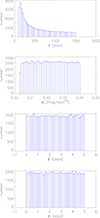 |
Fig. A.1. Distributions of the τ, σ, Δt, and σt of the N1 = 94527 artificial LC1(t) including fake QPOs. |
All Figures
|
Fig. 1. Correlation between SDSS g- and r-band apparent magnitudes of 3530 low-redshift quasars. The solid and dashed red lines show the best fitting results and corresponding 5σ confidence bands. |
| In the text | |
|
Fig. 2. Left panels: Light curves of LC1, 0(t) (in blue) and LC2, 0(t) (in red) (top left panel); LC1(t) (in blue) and LC2(t) (in red) (middle left panel); and Color(t) (bottom left panel). Right panels: Corresponding LS powers. In the top right panel (middle right panel), the solid line in blue and red show the results through LC1, 0(t) (LC1(t)) and LC2, 0(t) (LC2(t)), respectively. In each right panel, the horizontal dashed red line marks the 5σ significance level (determined by the input false alarm probability to be 3 × 10⁻⁷); the vertical dashed red line marks the position of periodicity around 812 days determined in LC1(t). |
| In the text | |
|
Fig. 3. Top panel: ZTF g-band (blue symbols) and r-band (red symbols) light curves of SDSS J1609+1756. Middle panel: CL(t). Bottom panel: Determined LS powers of CL(t). The horizontal dashed red line is the 5σ significance level. |
| In the text | |
|
Fig. A.1. Distributions of the τ, σ, Δt, and σt of the N1 = 94527 artificial LC1(t) including fake QPOs. |
| In the text | |
Current usage metrics show cumulative count of Article Views (full-text article views including HTML views, PDF and ePub downloads, according to the available data) and Abstracts Views on Vision4Press platform.
Data correspond to usage on the plateform after 2015. The current usage metrics is available 48-96 hours after online publication and is updated daily on week days.
Initial download of the metrics may take a while.