© The Authors 2025

1. Introduction

The current precession model recommended by the IAU is known as the IAU 2006 model (Capitaine et al. 2003). It is dynamically consistent with the IAU 2000 nutation and provides polynomial formulas for a number of angular quantities that are used in the GCRS-to-ITRS transformation paradigms. Recent studies show that different models of the Earth’s dynamical flattening H_d (in precession H_d is represented by a linear model, while in the nutation it is still a constant) is responsible for small inconsistency in the Earth’s rotation theory. To solve this problem, certain correction terms in nutation series were developed (see, e.g., Capitaine et al. 2005; Escapa et al. 2017).

As one part of the IAU 2006 model, the precession of the ecliptic was derived by fitting the analytical ephemerides VSOP87 (Bretagnon & Francou 1988) to the long-term numerical ephemerides DE406 (Standish 1998) over 2000 years. For the precession of the equator, the basic quantities ψ_A and ω_A were solved by integrating the dynamical precession equations of the equator based on the improved ecliptic precession and on the Williams (1994) expressions for the precession rates and the IAU 2000 integration constants (Mathews et al. 2002) corrected for a number of small perturbing effects (Capitaine et al. 2003).

A negative J₂ rate, which is generally attributed to the postglacial rebound of the Earth’s mantle, was adopted by the IAU 2006 precession of the equator: ${\dot{J}}_2=-3.001\times {10}^{-9}{\mathrm{cy}}^{-1}.$ This is a very important feature of the IAU 2006 model; however, the relative uncertainty of the ${\dot{J}}_2$ is about 20% (Williams 1994), and hence it is one of the main factors that limits the accuracy of the IAU 2006 precession model.

More recently, Liu & Capitaine (2017, denoted LC17 in the following) tried to construct an improved precession model by taking into account various advances in the Earth’s rotation theories and the Solar System ephemerides. In that work, new ephemerides DE422 (Folkner et al. 2009), INPOP10 (Fienga et al. 2011), and VSOP2013 (Simon et al. 2013) were incorporated to build the precession of the ecliptic. Several advances in theoretical precession rates, including contributions from revised nonlinear terms, tidal Poisson terms, second-order torque, Galactic aberration effect, and, more importantly, new determinations of the J₂ variation, were applied to derive the precession of the equator.

The LC17 solution has a clear difference for the quadratic and cubic terms in the polynomials of ψ_A. It shows a slight improvement with respect to the IAU 2006 precession as indicated by VLBI-observed celestial pole offsets (CPOs). Although adopted, the parabolic variation in the J₂ data up to 2012 was not firmly convincing. Due to the uncertainty in the J₂ empirical models and the limited time span of the VLBI observations, the authors recommended to retain the IAU 2006 model. In this paper, we resume our effort to improve the IAU precession model. Sect. 2 describes our investigation into the J₂ long-term variation with most recent satellite laser ranging (SLR) data, which is 13 years longer than that in LC17. In Sect. 3, the updated J₂ trend is used to integrate the precession equations. In Sect. 4 we check the updated precession against VLBI data over 45 years, for a comparison with the standard IAU 2006 model.

2. Long-term variation in the Earth’s J₂ parameter

Figure 1 shows the J₂ data points from 1976 to 2025, which were derived from the SLR observations of several geodetic satellites including LAGEOS-1 and -2, Starlette, Stella, as well as Ajisai. The original data description was given in Cheng et al. (2013)¹, and we note that the J₂ value was transformed from the original C₂₀ harmonic coefficient of the geopotential via simple relation $J_2=-\sqrt{5}{C}_{20}$. The data was provided for each 30 days, and thus we have a total of 597 data points for the following analysis.

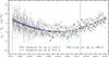Fig. 1. Earth’s J2 values evaluated from SLR and its long-term variation. The constant ${\overline{J}}_2$ is the mean value for J2, which equals 0.0010826359797. The original data with continuous updates to 2025 are provided by Cheng et al. (2013). The error bars are shown in gray. The green dashed line indicates the endpoint of the data that were used in LC17. The linear and parabolic fits within different time intervals are shown as colored curves.

The Earth’s oblateness is influenced by various geophysical processes, including the gradual slowing of its rotation due to tidal braking, large earthquakes, and ongoing post-glacial rebound. In the past years, the J₂ trend has been approximated by a negative linear drift attributed to postglacial rebound of the Earth’s mantle or the ongoing global isostatic adjustment (Yoder et al. 1983; Cox & Chao 2002), and therefore a constant J₂ rate was adopted in the IAU 2006 precession using data up to 1996 (straight blue line in Fig. 1). However, the value of J₂ tends to increase at around 2000. The disappearance of the negative trend is attributed to recent ice melt in the cryosphere, which altered the global mass distribution (see, e.g., Cheng & Ries 2018). At present, the SLR data spanning nearly 50 years demonstrates that the long-term variation of J₂ appears to be more quadratic than linear in nature (Cheng et al. 2013; Marchenko & Lopushanskyi 2018).

To explore the possibility of updating the precession model, LC17 adopted J₂ data from 1976 to 2012 (see the vertical dashed line in Fig. 1) and a parabola was used to interpret its long-term behavior. However, the quadratic feature at that time was not very convincing because the axis of symmetry is too close to the data ending. Having additional accurate J₂ data in the last 13 years, the nonlinear feature is visible with more clarity, and J₂ can be fit to a parabolic function with higher confidence. Using a weighted least-squares fit, the resulting J₂ variation is such that

$$\begin{array}{c}\hfill J_2=1.08263582\times {10}^{-3}-0.0778\times {10}^{-9}t+12.016\times {10}^{-9}{t}^2,\end{array}$$(1)

where t is Julian centuries elapsed from J2000.0. It can be found from the coefficients of t¹ (which indicate the symmetry axis position of the parabola) that the inflection point of J₂ changed a little bit because new data added. We note that the t¹ term of J₂ obtained in LC17 is about −0.5 × 10⁻⁹ cy⁻¹.

Using the coefficients of the empirical expression in Eq. (1), we derive the contribution of the J₂ variation to the precession rates in longitude, r_ψ (see Appendix A for the detailed procedure). The numerical values are listed in Table 1. The precision of the t² and t³ coefficients of r_ψ have been improved relative to LC17 by about 50% and 60%, respectively. The improvement percentage of the t² coefficient accuracy relative to the IAU 2006 model (∼78%) is even more remarkable.

3. Updated precession quantities consistent with the IAU 2006 model

The upgraded precession is developed with a semi-analytical approach similar to that used in Capitaine et al. (2003), and hence we regard the current study as an extension of LC17 in the framework of the IAU 2006 model. To emphasize the J₂ long-term model as the most important change, we consider it appropriate to name the new precession IAU 2006_J2. The updated solutions were obtained by integrating the differential equations (see Appendix B) using (i) the ecliptic precession P_A and Q_A derived from VSOP2013 and DE422, as given in LC17, and (ii) the theoretical contributions to the precession rates including the J₂ variation, as listed in line 3 of Table 1. Here we note that using the precession of the ecliptic from the latest ephemerides only produce a < 1 μas difference in the precession of the equator. To keep consistency with previous works and the IAU model, the polynomial expressions for P_A and Q_A from DE422 were retained (i.e. the upper part of Table 3 in LC17). The primary precession quantities, ψ_A and ω_A, of the updated solution IAU 2006_J2 are

$$\begin{array}{cc}\hfill {\psi }_{\mathrm{A}}& =5038\stackrel{″}{.}482041t-1\stackrel{″}{.}07182t^2+0\stackrel{″}{.}01754827t^3\hfill \\ \hfill & +0\stackrel{″}{.}000126577t^4-0\stackrel{″}{.}000000103t^5\hfill \\ \hfill {\omega }_{\mathrm{A}}& ={ϵ}_0-0\stackrel{″}{.}025754t+0\stackrel{″}{.}0512625t^2-0\stackrel{″}{.}0077249t^3\hfill \\ \hfill & -0\stackrel{″}{.}000000245t^4+0\stackrel{″}{.}000000260t^5,\hfill \end{array}$$(2)

with ${ϵ}_0=84381\stackrel{″}{.}406$ being the obliquity at the epoch of J2000.0. The secondary quantities p_A, ϵ_A, and χ_A are simultaneously derived and they are listed in Eq. (B.6).

The comparison of the precession quantities between the IAU 2006_J2 and IAU 2006 are listed in Table 2. The largest differences in the quadratic and cubic terms for ψ_A and p_A are attributed to the use of a very different empirical model for J₂ variation. The sign for the t³ term of ψ_A is now positive ($+0\stackrel{″}{.}01754827t^3$), whereas it is negative in the IAU 2006 ($-0\stackrel{″}{.}00114045t^3$). The precession in obliquity ω_A is very close to the IAU 2006 value because J₂ has no effect on this parameter: the only difference, at an order of 1 μ as cy⁻¹, originates from the ϵ-dependence of the theoretical effects used in LC17.

4. Comparison of the updated precession expressions with VLBI celestial pole offsets

Due to its unprecedented high accuracy, VLBI provides the best observational material to verify the precession–nutation models. Since 1980, the Earth orientation parameters are provided regularly by the International VLBI Service for Geodesy and Astrometry (IVS). For this work, we focused on the celestial pole offsets (CPOs) dX and dY, which represent the deviation of the standard IAU 2006/2000 model prediction from observations. To check the updated precession using VLBI data, the CPOs associated with the IAU 2006_J2 model (dX_IAUJ2, dY_IAUJ2) were required. To this end, a rigorous transformation method was implemented (see Appendix C).

4.1. Celestial pole offsets from VLBI observations

To date, thousands of 24h VLBI sessions have been analyzed, and the products of celestial pole offsets are published regularly by the IVS. As pointed out in Gattano et al. (2017), no CPO series from one specific analysis center has a clear advantage compared to the others. In this work we considered two typical CPO time series:² (1) the OPA2025a solution from the Paris observatory (7598 sessions from 1980.28 to 2025.63); and (2) the C04 data, which is the combined series (15213 sessions from 1984.03 to 2025.65). The comprehensive C04 provides interpolated data with a one-day interval, and thus it has a higher number of sessions. Both of the series take the IAU 2006/2000 precession–nutation as the reference model, and they can be converted to dX_IAUJ2 and dY_IAUJ2 using the procedure described in Appendix C.

As an example, we plot in Fig. 2 the dX time series from the OPA2025a solution. The IERS recommended model³ (Petit & Luzum 2010) was applied to remove the effect of free core nutation (FCN) in the CPO series. The original CPO series (corresponding to the IAU 2006 precession model) and the revised series (corresponding to the updated IAU 2006_J2 precession) are plotted in Panels (a) and (b), respectively. The formal error of the celestial pole offsets is the root sum square of the original VLBI error and the uncertainties of the FCN model. When comparing the upper and lower panels of Fig. 2, one can find that the curvature signal in the IAU 2006_J2 compatible series is clearly reduced, particularly at the end of the time interval. We expect that the deviation between two series will enlarge continuously in the coming decades.

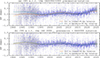Fig. 2. dX component of the celestial pole offsets after removing the free core nutation. Panel (a): CPO series referring to the reference model IAU 2006/2000A precession-nutation. Panel (b): CPO series with respect to the IAU 2006J2 precession plus IAU 2000A nutation (dXIAUJ2). The orange and green curves are fitted with Eq. (3; see Sect. 4.2 for more details).

The properties of the dY component is described briefly in Appendix D. There is no clear difference between the IAU 2006-compatible and IAU 2006_J2-compatible series, since the J₂ variation has almost no effect on ω_A, which dominates the Y coordinate of the CIP. In the following analysis, we mainly focus on the dX component that is affected intensively by the J₂ term.

Before going further, we tried to eliminate the effect of extreme outliers that are defined as |dX|> 20 mas. Consequently, 14 sessions from the OPA2025a data were excluded, and 7442 data points were retained. For the C04 series, no outlier was found. Table 3 provides the descriptive statistics for the CPO series corresponding the IAU 2006 and the IAU 2006_J2 precession models. The mean, weighted mean, and median values decrease very significantly if the updated IAU 2006_J2 expressions (Eqs. (2) and (B.6)) are adopted as the precession part of the Earth’s orientation model. This is true for the data from both CPO solutions, and therefore we arrived at the conclusion that the IAU 2006_J2 precession model is more consistent with the VLBI observations, in a global sense, than the present IAU 2006 model.

4.2. Comparison of precession models with VLBI

To interpret more deeply the properties of the residuals between the observations and different precession solutions, we adopted two empirical functions: (i) a straight line plus 18.6-year nutation, and (ii) a parabola plus the 18.6-year nutation, as in Capitaine et al. (2009) for the least-squares fits. The 18.6-year nutation is the largest nutation term and is expected to be sensitive to the errors of the secular precession model. The equations used for the fit of celestial pole offsets are such that

$$\begin{array}{c}\hfill \mathrm{d}X=\{\begin{array}{cc}\hfill A_0+A_{1}t+A_{\mathrm{s}}sin\mathrm{\Omega }+A_{\mathrm{c}}cos\mathrm{\Omega }& \hfill (\mathrm{i})\\ \hfill A_0+A_{1}t+A_2{t}^2+A_{\mathrm{s}}sin\mathrm{\Omega }+A_{\mathrm{c}}cos\mathrm{\Omega }& \hfill (\mathrm{ii}),\end{array}\end{array}$$(3)

where Ω is the mean longitude of the ascending node of the lunar orbit with a period of 18.6 years. The coefficients (A₀,  A₁,  A₂,  A_s,  A_c) in the two functions of Eq. (3), as well as the pre- and post-fit weighted root means squares (WRMS) of the residuals are demonstrated in Table 4. The fitted curves are plotted in orange and green in Fig. 2.

In Table 4, one can see pre-fit WRMS, which is another statistic to indicate the overall consistency between the observed CIP location and the theoretical prediction, is in all cases much smaller for the IAU 2006_J2 solution. The fitted coefficients are sensitive to the VLBI series, but generally the coefficients of most terms decreased obviously when the IAU 2006_J2 precession was employed, especially for the quadratic term from thousands of microarcseconds to the order of 15 and 364 μas. As expected, the residual coefficients for the main nutation term were also reduced by different amounts, particularly for the A_s value which decreased quite notably. In all cases, the post-fit WRMS are also 10% smaller for the CPO series when the IAU 2006_J2 precession is considered in data reduction. It should be kept in mind that the most important changes in our precession model is the introduction of an updated J₂ representation, leading to the reasonable inference that the use of J₂ quadratic variation eliminated most of the residual quadratic and long-period curvatures in the celestial pole offsets. A discussion of the correlation coefficients between the fitted parameters is presented in Appendix E.

5. Conclusion

In this study we investigated the possibility of improving the IAU 2006 precession model by updating the work of LC17. We introduced a more reliable parabolic function to model the long-term variation of J₂ based on accurate SLR observations over 50 years. It was implemented in the integration of the precession equations for the equator, with the same procedure as used in LC17. The new precession is named IAU 2006_J2. Since our approach is still in the framework of the IAU 2006 precession, we consider the present update as an IAU 2006 consistent model.

Table 2 shows that the quadratic and cubic terms in the precession in longitude, ψ_A, have differences on the order of 7.1 mas cy⁻² and 18.7 mas cy⁻³ with respect to the IAU 2006 model. With the help of the most accurate VLBI data in over 45 years, we tried to check and compare our precession models against state-of-the-art observations for the Earth’s rotation. The IAU 2006_J2 precession has shown clear advantages with respect to the IAU 2006 model (see Tables 3 and 4). Because a more realistic and accurate J₂ variation was applied, the IAU 2006_J2 solution shows better agreement to the real motion of the Earth in the GCRS, and will be more effective for predicting the CIP location in the GCRS. This is already so, as shown by the CPO series in recent years (see Fig. 2). Considering the improvements exhibited in the present work, we propose that the IAU 2006_J2 solution could be considered to replace the current standard model for the next update of the IERS Conventions. This work is also a contribution to the main objectives of the IAU/IAG Joint Working Group “Consistent Improvement of the Earth’s Rotation Theory (CIERT).” According to the updated precession, studies of the supplementary terms to the nutation series is necessary in order to ensure the consistency between precession (with varying H_d) and nutation (with constant H_d) models (Escapa et al. 2016, 2017; Ferrándiz et al. 2018).

Acknowledgments

We are grateful to Prof. Nicole Capitaine for valuable comments and discussion. We also thank the anonymous referee for his/her suggestions to improve the manuscript. This work is funded by the National Natural Science Foundation of China (NSFC) under grant Nos. 12373074 and 12233010.

References

Appendix A: The contribution of J₂ to the precession rate of the equator

According to the precession rate from the first order luni-solar term (e.g., Kinoshita & Souchay 1990), the effect of ${\dot{J}}_2$ is

$$\begin{array}{c}\hfill \frac{\mathrm{d}{r}_{\psi ,{\dot{J}}_2}}{\mathrm{d}t}=(\frac{{\dot{k}}_{\mathrm{M}}}{F_2^3}{M}_0+{\dot{k}}_{\mathrm{S}}{S}_0)cos{ϵ}_0,\end{array}$$(A.1)

where

$$\begin{array}{c}\hfill {\dot{k}}_{\mathrm{M}}=3{\dot{H}}_{\mathrm{d}}\frac{M_{\mathrm{M}}}{M_{\mathrm{M}}+M_{\mathrm{E}}}\frac{n_{\mathrm{M}}^2}{\omega },{\dot{k}}_{\mathrm{S}}=3{\dot{H}}_{\mathrm{d}}\frac{M_{\mathrm{S}}}{M_{\mathrm{S}}+M_{\mathrm{M}}+M_{\mathrm{E}}}\frac{n_{\mathrm{EM}}^2}{\omega }.\end{array}$$(A.2)

In Eqs. (A.1) and (A.2), the masses of the Moon, the Earth, and the Sun are denoted as M_M, M_E, and M_S, respectively. The subscript ‘EM’ means Earth-Moon. Here n_M denotes the mean motion of the Moon with respect to the Earth, n_EM the mean motion of the Earth-Moon barycenter with respect to the Sun, ω the mean angular velocity of the Earth, and F₂ a factor of mean Earth-Moon distance calculated from the spatial average about the orbital angle. The constant M₀ is (Kinoshita 1977)

$$\begin{array}{c}\hfill M_0=\frac{1}{4}(3{cos}^2{i}_{\mathrm{M}}-1){(1-e_{\mathrm{M}}^2)}^{-3/2}.\end{array}$$(A.3)

To calculate S₀, we just need to change i_M to i_EM = 0 and e_M to e_EM, where e and i are the eccentricity and the inclination, respectively. In Eq. (A.2), the Earth’s dynamical flattening H_d is

$$\begin{array}{c}\hfill H_{\mathrm{d}}=1-\frac{A+B}{2C},\end{array}$$(A.4)

which represents the ratio of the axial moment of inertia (C) to the equatorial moment of inertia (A and B). As shown in Bourda & Capitaine (2004), H_d is connected with J₂ via

$$\begin{array}{c}\hfill J_2=\frac{C}{M_{\mathrm{E}}{a}^2}{H}_{\mathrm{d}},\end{array}$$(A.5)

where a is the mean radius of the Earth.

To the first approximation, we can calculate the contribution of J₂ variation to the precession rate using Eq. (A.1) with an assumption that all of the quantities are constants except for the Earth’s global parameter J₂:

$$\begin{array}{c}\hfill \frac{\mathrm{d}{r}_{\psi ,{\dot{J}}_2}}{\mathrm{d}t}=3{\dot{J}}_2\frac{M_{\mathrm{E}}{a}^2}{C}(\frac{M_0}{F_2^3}·Q_{\mathrm{M}}+S_0·Q_{\mathrm{S}})·cos{ϵ}_0.\end{array}$$(A.6)

Here Q_M and Q_S are defined as

$$\begin{array}{c}\hfill Q_{\mathrm{M}}=\frac{M_{\mathrm{M}}}{M_{\mathrm{M}}+M_{\mathrm{E}}}\frac{n_{\mathrm{M}}^2}{\omega },Q_{\mathrm{S}}=\frac{M_{\mathrm{S}}}{M_{\mathrm{S}}+M_{\mathrm{M}}+M_{\mathrm{E}}}\frac{n_{\mathrm{EM}}^2}{\omega }.\end{array}$$(A.7)

This is also the procedure adopted by Kinoshita & Souchay (1990) and Williams (1994).

Appendix B: The dynamical equations for the precession of the equator

The dynamical equations for solving the primary precession quantities ψ_A and ω_A can be found in Capitaine et al. (2003):

$$\begin{array}{cc}\hfill sin{\omega }_{\mathrm{A}}\frac{\mathrm{d}{\psi }_{\mathrm{A}}}{\mathrm{d}t}& =(r_{\psi }sin{ϵ}_{\mathrm{A}})cos{\chi }_{\mathrm{A}}-r_{ϵ}sin{\chi }_{\mathrm{A}},\hfill \\ \hfill \frac{\mathrm{d}{\omega }_{\mathrm{A}}}{\mathrm{d}t}& =r_{ϵ}cos{\chi }_{\mathrm{A}}+(r_{\psi }sin{ϵ}_{\mathrm{A}})sin{\chi }_{\mathrm{A}}.\hfill \end{array}$$(B.1)

Here r_ψ and r_ϵ are theoretical precession rates including the contribution of J₂. The other two precession angles p_A (general precession) and ϵ_A (obliquity of date) depend on the precession of the ecliptic P_A and Q_A,

$$\begin{array}{cc}\hfill \frac{\mathrm{d}{p}_{\mathrm{A}}}{\mathrm{d}t}& =r_{\psi }-cot{ϵ}_{\mathrm{A}}(A·sin{p}_{\mathrm{A}}+B·cos{p}_{\mathrm{A}})-2C\hfill \\ \hfill \frac{\mathrm{d}{ϵ}_{\mathrm{A}}}{\mathrm{d}t}& =r_{ϵ}-B·sin{p}_A+A·cos{p}_{\mathrm{A}},\hfill \end{array}$$(B.2)

where A, B, and C are functions of variables p and q:

$$\begin{array}{cc}\hfill A(p,q)& =r[\dot{q}+p(q\dot{p}-p\dot{q})],\hfill \\ \hfill B(p,q)& =r[\dot{p}-q(q\dot{p}-p\dot{q})],\hfill \\ \hfill C(p,q)& =q\dot{p}-p\dot{q},\hfill \end{array}$$(B.3)

with $r=2/\sqrt{1-p^2-q^2}$. The parameters p and q are alternative representations of the precession of the ecliptic

$$\begin{array}{c}\hfill p=\frac{P_{\mathrm{A}}}{2\sqrt{1-P_{\mathrm{A}}^2-Q_{\mathrm{A}}^2}};q=\frac{Q_{\mathrm{A}}}{2\sqrt{1-P_{\mathrm{A}}^2-Q_{\mathrm{A}}^2}},\end{array}$$(B.4)

with P_A and Q_A being polynomials of t. They can be found in Tables 2 and 3 of the LC17 paper. The last quantity χ_A (precession of the ecliptic measured along the mean equator of date) is derived from geometric relation:

$$\begin{array}{c}\hfill sin{\chi }_{\mathrm{A}}sin{\omega }_{\mathrm{A}}=P_{\mathrm{A}}cos{p}_{\mathrm{A}}+Q_{\mathrm{A}}sin{p}_{\mathrm{A}}.\end{array}$$(B.5)

As done in LC17, the 7(8)-degree Runge-Kutta-Fehlberg (RKF) method is employed to integrate Eqs. (B.1−B.5) in the time interval of J1000 to J3000. Except for the main quantities ψ_A and ω_A in Eq. (2), the secondary quantities p_A, ϵ_A, and χ_A are simultaneously derived:

$$\begin{array}{cc}\hfill p_{\mathrm{A}}& ={5028}^{″}.796900t+1^{″}.1125525t^2+0^{″}.0187702t^3\hfill \\ \hfill & -0^{″}.000019662t^4-0^{″}.000000017t^5,\hfill \\ \hfill {ϵ}_{\mathrm{A}}& ={ϵ}_0-{46}^{″}.836734t-0^{″}.0001936t^2+0^{″}.00200004t^3\hfill \\ \hfill & -0^{″}.000000602t^4+0^{″}.000000011t^5,\hfill \\ \hfill {\chi }_{\mathrm{A}}& ={10}^{″}.556240t-2^{″}.3813876t^2-0^{″}.00121400t^3\hfill \\ \hfill & +0^{″}.000159277t^4-0^{″}.000000087t^5.\hfill \end{array}$$(B.6)

Appendix C: Celestial pole offsets associated with the IAU 2006_J2 precession model

According the definition of celestial pole offsets, the observed CIP coordinates in the GCRS can be written as

$$\begin{array}{c}\hfill X_{\mathrm{obs}}=X_{\mathrm{IAU}}+\mathrm{d}{X}_{\mathrm{IAU}},Y_{\mathrm{obs}}=Y_{\mathrm{IAU}}+\mathrm{d}{Y}_{\mathrm{IAU}},\end{array}$$(C.1)

where the subscript IAU means that the reference model is the IAU 2006/2000A. To verify our updated precession model using VLBI data, the celestial pole offsets compatible with the IAU 2006_J2 precession solution is needed. The procedure for this purpose was introduced in Capitaine & Wallace (2006).

As the first step, we form the precession matrix ${\mathcal{P}}_{{\mathrm{IAU}}_{J_2}}$ associated with the IAU 2006_J2 model in Eqs. (2) and (B.6),

$$\begin{array}{c}\hfill {\mathcal{P}}_{{\mathrm{IAU}}_{J_2}}={\mathcal{R}}_3({\chi }_{\mathrm{A}})·{\mathcal{R}}_1(-{\omega }_{\mathrm{A}})·{\mathcal{R}}_3(-{\psi }_{\mathrm{A}})·{\mathcal{R}}_1({ϵ}_0),\end{array}$$(C.2)

where ℛ₁, ℛ₂, and ℛ₃ are rotation matrices around the x-, y-, and z-axes, respectively. This classical four-rotation transformation method makes use of the original quantities derived from the dynamical solutions. The advantage is that it can separate distinctly precession of the ecliptic and precession of the equator.

Then the bias-precession-nutation matrix ${\mathcal{M}}_{{\mathrm{IAU}}_{J_2}}$ is calculated using the IAU 2000A_R06 nutation matrix 𝒩 and the frame bias matrix ℬ at J2000.0:

$$\begin{array}{c}\hfill {\mathcal{M}}_{{\mathrm{IAU}}_{J_2}}=\mathcal{N}·{\mathcal{P}}_{{\mathrm{IAU}}_{J_2}}·\mathcal{B}.\end{array}$$(C.3)

In the above equation, the frame bias matrix

$$\begin{array}{c}\hfill \mathcal{B}={\mathcal{R}}_1(-{\eta }_0)·{\mathcal{R}}_2({\xi }_0)·{\mathcal{R}}_3(\mathrm{d}{\alpha }_0)\end{array}$$(C.4)

specifies the constant orientation offset between the ICRS and the J2000.0 mean equatorial reference system. Here η₀ = −16.617 ± 0.01 mas and ξ₀ = −6.819 ± 0.01 mas are the coordinates of the CIP at J2000.0 in the GCRS, and dα₀ = −14.6 ± 0.5 mas is the equinox offset between the two reference systems. The nutation matrix 𝒩 is written as

$$\begin{array}{c}\hfill \mathcal{N}={\mathcal{R}}_1(-[{ϵ}_{\mathrm{A}}+\mathrm{\Delta }ϵ])·{\mathcal{R}}_3(-\mathrm{\Delta }\psi )·{\mathcal{R}}_1({ϵ}_{\mathrm{A}}),\end{array}$$(C.5)

where the Δψ and Δϵ are the nutation angles in longitude and obliquity with respect to the moving ecliptic. The IAU 2000A nutation series (Mathews et al. 2002) with adjustments of IAU 2006 precession is applied.

In the next step, the CIP coordinates corresponding to the IAU 2006_J2 precession are extracted from the [3, 1] and [3, 2] elements of the matrix ${\mathcal{M}}_{{\mathrm{IAU}}_{J_2}}$:

$$\begin{array}{c}\hfill X_{{\mathrm{IAU}}_{J_2}}={\mathcal{M}}_{{\mathrm{IAU}}_{J_2}}[3,1];Y_{{\mathrm{IAU}}_{J_2}}={\mathcal{M}}_{{\mathrm{IAU}}_{J_2}}[3,2].\end{array}$$(C.6)

This is due to the fact that (IERS Conventions 2010, Petit & Luzum 2010):

$$\begin{array}{c}\hfill {\mathcal{M}}_{{\mathrm{IAU}}_{J_2}}=\left(\begin{array}{ccc}1-a{X}^2& -aXY& -X\\ -aXY& 1-a{Y}^2& -Y\\ X& Y& 1-a(X^2+Y^2)\end{array}\right),\end{array}$$(C.7)

in which a ≃ 1/2 + (X² + Y²)/8. Here the subscript IAU_J2 for all of the X and Y coordinates are omitted for brevity.

Finally, the theoretical predictions of X_IAUJ2 and Y_IAUJ2 are subtracted from the observed CIP coordinates to get the new celestial pole offsets,

$$\begin{array}{c}\hfill \mathrm{d}{X}_{{\mathrm{IAU}}_{J_2}}=X_{\mathrm{obs}}-X_{{\mathrm{IAU}}_{J_2}},\mathrm{d}{Y}_{{\mathrm{IAU}}_{J_2}}=Y_{\mathrm{obs}}-Y_{{\mathrm{IAU}}_{J_2}},\end{array}$$(C.8)

with X_obs and Y_obs being derived from Eq. (C.1). The IAU SOFA software package⁴ (Standard of Fundamental Astronomy,Hohenkerk 2012) was employed for the above calculations. The transformed CPO series correspding to the IAU 2006_J2 precession (dX_IAUJ2, dY_IAUJ2) will be analyzed in Sect. 4.

Appendix D: Brief results for the dY component

Since J₂ has no contribution to the precession of the obliquity ω_A, the CIP coordinate Y merely has changes on the order of several microarcseconds (see Table 2). As a result, the dY component of the celestial pole offsets remains almost the same when different precession has been considered (see Fig. D.1). We only give out simple statistical information for the OPA2025a series: the mean, weighted mean, and the median value for the dY component of the celestial pole offsets (FCN removed using the model in Petit & Luzum 2010), are 20 μas, 77 μas, and −84 μas, respectively. If, for example, a weighted fit of a model comprising a parabola plus a correction to the 18.6-year periodic term was conducted, we get the coefficients: A₀ = −90, A₁ = −86, A₂ = 554, A_s = 16, and A_c = −62 μas. In general, the magnitude of these numbers are in agreement with those derived from the dX component.

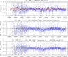Fig. D.1. The dY component of CPO series from the OPA2025a solution. Panel (a) shows the original CPOs and the empirical FCN model (the red curve). Panels (b) and (c) are the CPOs after removing the FCN effect, corresponding to the IAU 2006J2 and the IAU 2006 precession models, respectively.

Appendix E: Correlation coefficients for the parameters in Table 4

The coefficients of correlation associated with the least squares fits using the C04 series (see Table 4) are summarized in Table E.1. Generally they are quite small. In the fit of a linear plus nutation term, the correlation coefficient is on the order of 0.6 between the constant and linear term, and the correlation between linear term and nutation sine term is also pronounced. For the fit using function (ii) in Eq. (3), we have strong correlation (∼0.7) between linear and quadratic term. This may be attributed to the fact that precession itself is a motion with a period of ∼26 000 years, while the time span of the VLBI data is still not long enough to fully interpret the nature of the residuals. However, at a global level, the correlations for nutation terms are weak, indicating that the VLBI data is now capable of separating the precession and nutation parts from the motion of the CIP. We note that the results for the OPA2025a solution is quite similar to C04.

All Tables

All Figures

Fig. 1. Earth’s J2 values evaluated from SLR and its long-term variation. The constant ${\overline{J}}_2$ is the mean value for J2, which equals 0.0010826359797. The original data with continuous updates to 2025 are provided by Cheng et al. (2013). The error bars are shown in gray. The green dashed line indicates the endpoint of the data that were used in LC17. The linear and parabolic fits within different time intervals are shown as colored curves.

In the text

	Fig. 2. dX component of the celestial pole offsets after removing the free core nutation. Panel (a): CPO series referring to the reference model IAU 2006/2000A precession-nutation. Panel (b): CPO series with respect to the IAU 2006J2 precession plus IAU 2000A nutation (dXIAUJ2). The orange and green curves are fitted with Eq. (3; see Sect. 4.2 for more details).
In the text

	Fig. D.1. The dY component of CPO series from the OPA2025a solution. Panel (a) shows the original CPOs and the empirical FCN model (the red curve). Panels (b) and (c) are the CPOs after removing the FCN effect, corresponding to the IAU 2006J2 and the IAU 2006 precession models, respectively.
In the text

References

- Bourda, G., & Capitaine, N. 2004, A&A, 428, 691 [NASA ADS] [CrossRef] [EDP Sciences] [Google Scholar]
- Bretagnon, P., & Francou, G. 1988, A&A, 202, 309 [NASA ADS] [Google Scholar]
- Capitaine, N., & Wallace, P. T. 2006, A&A, 450, 855 [NASA ADS] [CrossRef] [EDP Sciences] [Google Scholar]
- Capitaine, N., Wallace, P. T., & Chapront, J. 2003, A&A, 412, 567 [NASA ADS] [CrossRef] [EDP Sciences] [Google Scholar]
- Capitaine, N., Wallace, P. T., & Chapront, J. 2005, A&A, 432, 355 [NASA ADS] [CrossRef] [EDP Sciences] [Google Scholar]
- Capitaine, N., Mathews, P. M., Dehant, V., Wallace, P. T., & Lambert, S. B. 2009, CeMDA, 103, 179 [Google Scholar]
- Cheng, M., & Ries, J. C. 2018, Geophys. J. Int., 212, 1218 [Google Scholar]
- Cheng, M., Tapley, B. D., & Ries, J. C. 2013, J. Geophys. Res. (Solid Earth), 118, 740 [Google Scholar]
- Cox, C. M., & Chao, B. F. 2002, Science, 297, 831 [Google Scholar]
- Escapa, A., Ferrándiz, J. M., Baenas, T., et al. 2016, Pure Appl. Geophys., 173, 861 [Google Scholar]
- Escapa, A., Getino, J., Ferrándiz, J. M., & Baenas, T. 2017, A&A, 604, A92 [NASA ADS] [CrossRef] [EDP Sciences] [Google Scholar]
- Ferrándiz, J. M., Navarro, J. F., Martínez-Belda, M. C., Escapa, A., & Getino, J. 2018, A&A, 618, A69 [NASA ADS] [CrossRef] [EDP Sciences] [Google Scholar]
- Fienga, A., Laskar, J., Kuchynka, P., et al. 2011, Celest. Mech. Dyn. Astron., 111, 363 [Google Scholar]
- Folkner, W. M., Williams, J. G., & Boggs, D. H. 2009, Interplanet. Network Prog. Rep., 42-178, 1 [Google Scholar]
- Gattano, C., Lambert, S. B., & Bizouard, C. 2017, J. Geod., 91, 849 [NASA ADS] [CrossRef] [Google Scholar]
- Hohenkerk, C. 2012, in IAU SOFA Software, IAU Joint Discussion, P23 [Google Scholar]
- Kinoshita, H. 1977, Celest. Mech., 15, 277 [Google Scholar]
- Kinoshita, H., & Souchay, J. 1990, CeMDA, 48, 187 [Google Scholar]
- Liu, J. C., & Capitaine, N. 2017, A&A, 597, A83 (LC17) [NASA ADS] [CrossRef] [EDP Sciences] [Google Scholar]
- Marchenko, A., & Lopushanskyi, O. 2018, Geodynamics, 2, 5 [Google Scholar]
- Mathews, P. M., Herring, T. A., & Buffett, B. A. 2002, J. Geophys. Res. (Solid Earth), 107, 2068 [NASA ADS] [CrossRef] [Google Scholar]
- Petit, G., & Luzum, B. 2010, IERS conventions (2010), Bundesamt für Kartographie und Geodäsie Frankfurt am Main, Germany [Google Scholar]
- Simon, J. L., Francou, G., Fienga, A., & Manche, H. 2013, A&A, 557, A49 [NASA ADS] [CrossRef] [EDP Sciences] [Google Scholar]
- Standish, E. M. 1998, Interoffice memorandum: JPL IOM 312. F - 98-048 [Google Scholar]
- Williams, J. G. 1994, AJ, 108, 711 [Google Scholar]
- Yoder, C. F., Williams, J. G., Dickey, J. O., et al. 1983, Nature, 303, 757 [Google Scholar]
Appendix A: The contribution of J2 to the precession rate of the equator