| Issue |
A&A
Volume 704, December 2025
|
|
|---|---|---|
| Article Number | A101 | |
| Number of page(s) | 16 | |
| Section | Extragalactic astronomy | |
| DOI | https://doi.org/10.1051/0004-6361/202452055 | |
| Published online | 03 December 2025 | |
Enhanced active galactic nucleus activity in overdense galactic environments at 2 < z < 4
1
Department of Physics and Astronomy, University of California, Davis, One Shields Avenue, Davis, CA 95616, USA
2
Gemini Observatory, NSF NOIRLab, 670 N. A’ohoku Place, Hilo, HI 96720, USA
3
Space Telescope Science Institute, Baltimore, MD 21218, USA
4
Department of Physics and Astronomy, Texas A & M University, College Station, TX 77843-4242, USA
5
INAF-Osservatorio di Astrofisica e Scienza dello Spazio, Via Gobetti 93/3, I-40129 Bologna, Italy
6
University of Hawai’i, Institute for Astronomy, 2680 Woodlawn Drive, Honolulu, HI 96822, USA
7
Department of Astronomy, Tsinghua University, Beijing 100084, China
8
INAF – Osservatorio astronomico di Padova, Vicolo Osservatorio 5, 35122 Padova, Italy
9
INAF-IASF Milano, Via Alfonso Corti 12, 20133 Milano, Italy
10
University of Bologna – Department of Physics and Astronomy “Augusto Righi” (DIFA), Via Gobetti 93/2, 40129 Bologna, Italy
11
SISSA, Via Bonomea 265, I-34136 Trieste, Italy
12
IFPU – Institute for fundamental physics of the Universe, Via Beirut 2, 34014 Trieste, Italy
⋆ Corresponding author: This email address is being protected from spambots. You need JavaScript enabled to view it.
Received:
30
August
2024
Accepted:
25
August
2025
Abstract
We carried out a study on the relationship between galaxy environments and their active galactic nucleus (AGN) activity at high redshifts (2.0 < z < 4.0). Specifically, we studied the AGN fraction in galaxies residing in a range of environments at these redshifts, from field galaxies to the densest regions of highly overdense peaks in the GOODS-S extragalactic field. Utilizing the extensive photometric and spectroscopic observations in this field, we measured the local overdensities (σδ) and global overdensities across a broad a range of environments, including those in massive (Mtot ≥ 1014.8 M⊙) protostructures. We employed a multiwavelength AGN catalog consisting of AGNs in nine different categories. Our analysis shows a higher AGN fraction (10.9−2.3+3.6%) for galaxies in the highest local overdensity regions compared to the AGN fraction (1.9−0.3+0.4%) in the corresponding coeval field galaxies (a ∼4σ difference). This trend of increasing AGN fraction in denser environments relative to the field is present in all redshift bins. We also find this trend to be consistent across all five AGN categories that have a sufficient number of AGNs to make a meaningful comparison: the mid-infrared (MIR) spectral energy distribution (SED), MIR color, X-ray luminosity, X-ray-luminosity-to-radio-luminosity-ratio, and optical-spectroscopy. Our results also demonstrate a clear trend for higher (∼4×) AGN fractions in denser local overdensity environments for a given stellar mass. Additionally, we observe the same trend (though at a lower significance) with the global environment of galaxies, measured using a metric based on the projected distance of galaxies from their nearest massive (Mtot > 1012.8 M⊙) overdense (σδ > 5.0) peak, normalized with respect to the size of the peak. These findings indicate that the prevalence of AGN activity is highly dependent on the environment a host galaxy resides in, even at early times in the formation history of the Universe.
Key words: galaxies: active / galaxies: evolution / galaxies: high-redshift / galaxies: nuclei / galaxies: structure / large-scale structure of Universe
© The Authors 2025
 Open Access article, published by EDP Sciences, under the terms of the Creative Commons Attribution License (https://creativecommons.org/licenses/by/4.0), which permits unrestricted use, distribution, and reproduction in any medium, provided the original work is properly cited.
This article is published in open access under the Subscribe to Open model. This email address is being protected from spambots. You need JavaScript enabled to view it. to support open access publication.
1. Introduction
Galaxies are found in a variety of environments, ranging from sparsely populated field regions where galaxies have very few neighbors to dense galaxy clusters in which thousands of galaxies can reside in a relatively small region. The environment of a galaxy plays a crucial role in its formation and evolution. The gravitational potential well of large dense structures affect the motion of galaxies as well as their interaction and merger rate with other galaxies (Kim et al. 2024). For these reasons and many others, large dense structures can significantly alter the properties of their constituent galaxies such as morphology, stellar mass, star formation rate (SFR), and active galactic nuclei (AGN) activity (Dressler 1980; Balogh et al. 2000; Edler et al. 2024; Rihtaršič et al. 2024), as well as a number of other properties.
The term AGN refers to the supermassive black hole (SMBH) at the center of a galaxy that is actively accreting matter and emitting intense radiation. As more material gets accreted onto a SMBH, it grows, eventually leading to a triggering of the AGN (e.g., Silk & Rees 1998; Fabian 1999). The feedback caused by AGN emission can affect the properties of galaxies such as its star formation (e.g., Silk & Rees 1998; Di Matteo et al. 2005; Belli et al. 2024), morphology (e.g., Dubois et al. 2016), and chemical enrichment of the intragalactic medium (e.g., Hamann & Ferland 1999; Bower et al. 2008; Kara et al. 2024) among many other properties. Therefore, the interplay between black hole growth and AGN feedback is a critical aspect of galaxy evolution as it connects the growth of the black hole to the properties and evolution of the host galaxy.
AGNs are typically classified into various categories based on their observed properties. For example, radio-loud AGNs emit strong radio waves relative to the strength of emission in other bandpasses (typically optical), likely due to the presence of relativistic jets powered by the central SMBH. Radio-quiet AGNs have weaker radio emission, possibly due to the absence or weakness of these jets (e.g., Urry & Padovani 1995; Wilson & Colbert 1995). Based on optical spectra, AGNs with broad emission lines (known as type I) are thought to provide a direct view of the central engine of the AGN and broad-line region, whereas type II AGNs, which exhibit narrow emission lines, are thought to be viewed through an optically thick dusty torus that obscures the central engine and broad-line region (e.g., Ramos Almeida et al. 2011; Villarroel & Korn 2014). The re-radiation of absorbed light from dust surrounding the AGN can cause an infrared-bright (IR-bright) AGNs (e.g., Stern et al. 2005; Donley et al. 2012). Some types of AGN can also be identified by their strong X-ray emission (e.g., Rees 1984; Ueda et al. 2003; Buchner et al. 2014). Among the most extreme examples of AGN are quasars, which are so luminous that they often outshine their host galaxies (e.g., Antonucci 1993; Urry & Padovani 1995; Silk & Rees 1998). Additionally, the “little red dots” observed by the James Webb Space Telescope (JWST) could represent a population of heavily obscured, high-redshift AGNs, providing insights into early black hole growth (e.g., Matthee et al. 2024). Different processes may be responsible for triggering different types of AGN. Since an AGN identified using one criterion does not necessarily meet the criteria in all other categories simultaneously, the results of AGN studies can vary depending on the type of AGN considered.
Galaxy interactions and mergers can have profound impacts on the evolution of galaxies, affecting their morphology, gas content, and star formation histories (SFHs, e.g., Barnes & Hernquist 1991; Mihos & Hernquist 1996; Lotz et al. 2008; Ellison et al. 2010). In particular, the relationship between mergers and AGNs has been studied extensively over cosmic time (e.g., Sanders et al. 1988; Alonso et al. 2007; Ellison et al. 2011; Hopkins & Quataert 2011; Silverman et al. 2011; Donley et al. 2018; Blecha et al. 2018). Theoretical models suggest that the gravitational torques arising from interactions can funnel large amounts of cold gas into the nuclear regions, thus enhancing black-hole accretion and boosting AGN activity (e.g., Kawakatu et al. 2006; Hopkins & Quataert 2011). This scenario appears to hold in many studies of low-z galaxies which find significant AGN enhancement in close pairs or merging galaxies (e.g., Ellison et al. 2013; Satyapal et al. 2014; Ellison et al. 2019).
However, other observational works have suggested that a large fraction of AGNs – particularly moderate-luminosity and/or high-redshift (z ∼ 1.5 − 2.5) AGNs – are triggered by mechanisms that are not typically associated with major mergers, such as disk instabilities or stochastic processes (e.g., Cisternas et al. 2011; Kocevski et al. 2012). Additionally, the timescales for AGN visibility may not align perfectly with mergers and dust obscuration (especially at higher redshift) could complicate the observational studies (e.g., Hopkins & Quataert 2011). At even higher redshifts (z ≳ 2), the role of mergers and dense environments in triggering AGNs becomes even more uncertain. Some studies have found enhanced AGN fractions in protoclusters or close galaxy systems at z > 1 − 2 (e.g., Digby-North et al. 2010; Polletta et al. 2021; Monson et al. 2023), while others have reported little to no difference in AGN incidence between merging and isolated galaxies (e.g., Macuga et al. 2019; Shah et al. 2020). While large gas fractions in early galaxies could, in principle, promote merger-driven inflows (e.g., Kawakatu et al. 2006), increased turbulence and shorter dynamical timescales may counteract these inflows and suppress AGN fueling (e.g., Di Matteo et al. 2008; Fensch et al. 2017).
Another challenge is the complex interplay between local (i.e., small-scale, galaxy-galaxy) environments and global (cluster-scale or proto-cluster) environments. Galaxy-scale interactions and mergers can drive immediate gas inflows, while large-scale cluster membership can influence halo gas reservoirs or accretion modes over longer timescales (Koulouridis et al. 2013). By comparing local overdensity (e.g., close pairs) with global overdensity (e.g., distance from a massive cluster), we can begin to discern the relative roles of small-scale interactions versus cluster-scale processes in AGN triggering.
The complex connection of AGN activity and dense environments of galaxy clusters has been studied in depth at low-to-intermediate redshifts (z ≲ 1.5). In the Local Universe, observational studies show that luminous AGNs are fractionally less common among cluster galaxies compared to coeval field galaxies (Kauffmann et al. 2004; Popesso & Biviano 2006), while the population of less luminous AGN does not show a significant difference with environment (Martini et al. 2002; Miller et al. 2003; Martini et al. 2006; Haggard et al. 2010). Best (2004) found that AGNs are preferentially found in large-scale environments (such as moderate groups and clusters) compared to the local environment of the galaxy. At 0.65 < z < 0.96, Shen et al. (2017) show that radio-AGNs are more likely to be found in dense local environments of the large-scale structures (LSSs) identified as a part of the Observations of Redshift Evolution in the Large-Scale Environments (ORELSE) survey (Lubin et al. 2009). However, at 1 < z < 1.5, Martini et al. (2013) show consistent X-ray and mid-IR (MIR) selected AGN fractions in the clusters and field. Some studies show a significant decrement in the fraction of X-ray AGNs with a decreasing cluster-centric radius, from r500 to the central regions (e.g., Ehlert et al. 2013; Pentericci et al. 2013; Koulouridis et al. 2024). Additionally, at 0.65 < z < 1.28, Rumbaugh et al. (2017) generally did not observe any strong connection between AGN activity and location within the LSSs in the ORELSE survey. However, they observed a notable exception in two dynamically most unrelaxed LSSs (SG0023 and SC1604), where there was an overabundance of kinematic pairs, suggesting that merging activity could be a significant factor in AGN triggering. This highlights that at least some LSS environments might play a role in triggering AGN activity through merging processes at these redshifts. Some studies show higher AGN fractions in groups compared to clusters at low z (z < 0.5) (Arnold et al. 2009; Koulouridis et al. 2018). On the other hand, studies such as Klesman & Sarajedini (2012) did not report any significant correlations between AGN activity and cluster properties such as mass, X-ray luminosity, size, morphology, and redshift at 0.5 < z < 0.9 in their sample of AGNs identified based on optical variability, X-ray emission, or MIR power-law spectral energy distributions (MIR SEDs).
The complexity of the relation between dense environments of galaxies and their AGN activity is in some ways heightened at high redshift. Some studies on individual protoclusters, such as Krishnan et al. (2017) (X-ray AGNs; z ∼ 1.7), Tozzi et al. (2022) (X-ray AGNs; z ∼ 2.156), Digby-North et al. (2010) (AGN identification using emission-lines in optical/near-IR (optical/NIR) spectra; z ∼ 2.2), and Monson et al. (2023) (X-ray AGNs; z ∼ 3.09) show enhanced AGN activity among galaxies inhabiting protoclusters as compared to their field counterparts. Lemaux et al. (2014) showed a strong AGN activity in the brightest protocluster galaxy of Cl J0227-0421 at z ∼ 3.3. However, other studies, such as that of Macuga et al. (2019) (X-ray AGNs; z ∼ 2.53), do not show this same trend. Similarly, Lemaux et al. (2018) did not see any AGN activity in member galaxies of a massive protocluster at z ∼ 4.57. A large sample of protostructures1 over a large redshift range is required to understand the overall nature of this trend. Furthermore, as highlighted in Hashiguchi et al. (2023), populations of various types of AGN should be used to study the environment-AGN connection. Each type of AGN provides unique insights into different aspects of AGN activity, revealing information such as the central engine, obscuring structures, and the interaction of an AGN with its surroundings. A diverse approach encapsulating different types of AGN is key for capturing a broad spectrum of AGN phenomena across various redshifts. However, achieving this across a large redshift range requires deep, multiwavelength observations, which are challenging due to the faintness of distant sources and the extensive multiwavelength observational resources needed. These requirements make studying the environment-AGN connection at high redshift challenging.
Utilizing the vast amount of deep multiwavelength data in the Great Observatories Origins Deep Survey – South (GOODS-S) extragalactic field (Giavalisco et al. 2004) and the CANDELS survey (Grogin et al. 2011; Koekemoer et al. 2011), we were able to study the connection of environment and AGN activity of galaxies at 2 < z < 4. We used a large sample of spectroscopically and photometrically selected galaxies spanning a wide range of environments, from field to protostructures, with the latter including five of the spectroscopically confirmed massive protostructures presented in Shah et al. (2024), as well as a large number of other massive protostructures. We used a novel environmental measurement technique, which allowed us to define a coeval sample of field galaxies along with the samples of galaxies in denser environments. For the AGN identification, we employed the AGN catalog presented in Lyu et al. (2022), which uses deep multiwavelength observations from X-ray to radio to provide AGN samples in nine different categories. These samples of galaxies and AGNs enable us to conduct an unprecedented study on the environment-AGN connection of galaxies during an important epoch (2 < z < 4) of the cosmic history.
The layout of this paper is as follows. We describe the data and methods used for generating the galaxy and AGN samples in Sect. 2. In Sect. 3, we present our analysis on the change in the AGN fraction with environment overdensity. We discuss our results and compare them with other studies in Sect. 4. Lastly, we summarize our results in Sect. 5.
2. Data and methods
In this section, we provide the details of the observations and methods used to generate the galaxy sample (Sect. 2.1) and the AGN sample (Sect. 2.2). We then describe the spectral energy distribution (SED) fitting process used to estimate the stellar masses of galaxies in Sect. 2.3 and the Voronoi Monte Carlo mapping method used to measure the local overdensity of galaxies in Sect. 2.4.
2.1. Galaxy sample
In this study, we utilized2 the extensive photometric (Sect. 2.1.1) and spectroscopic (Sect. 2.1.2) observations in the Extended Chandra Deep Field South (ECDFS) field (Lehmer et al. 2005), which encapsulated the GOODS-S field. The ECDFS field has deep multiwavelength observations available across the electromagnetic spectrum (e.g., Zheng et al. 2004; Wuyts et al. 2008; Cardamone et al. 2010; Dahlen et al. 2013; Hsu et al. 2014) enabling a wide range of extragalactic studies (e.g., Kaviraj et al. 2008; Le Fèvre et al. 2015; Marchi et al. 2018; Birkin et al. 2021).
2.1.1. Photometric catalog
To generate the initial galaxy sample, we selected galaxies from the Cardamone et al. (2010) photometric catalog for galaxies in the ECDFS field. This catalog includes deep optical medium-band photometry (18 bands) from the Subaru telescope, UBVRIz photometry from the Garching-Bonn Deep Survey (GaBoDS; Hildebrandt et al. 2006) and the Multiwavelength Survey by Yale-Chile (MUSYC; Gawiser et al. 2006) survey, as well as deep NIR imaging in JHK from MUSYC (Moy et al. 2003), and Spitzer Infrared Array Camera (IRAC) photometry obtained using the Spitzer IRAC/MUSYC Public Legacy Survey in ECDFS (SIMPLE; Damen et al. 2011). The multiwavelength observations used for generating the galaxy catalogs, estimating the stellar masses of galaxies using spectral energy distribution, and utilizing the Voronoi Monte Carlo (VMC) mapping technique to calculate the overdensity values for galaxies are described in detail in Shah et al. (2024).
For this study, we only selected only the galaxies which have their IRAC1 (3.6 μm band) or IRAC2 (4.5 μm band) magnitudes brighter than 24.8. The selection of this cutoff was determined by considering the 3σ limiting depth of the IRAC images within the ECDFS field. This cut ensures a reliable detection in the rest-frame optical wavelengths at these redshifts, which helps constrain the Balmer/4000 Å break for galaxies at 2 < z < 5 (see Lemaux et al. 2018 for details). There are 55,147 unique objects in our sample satisfying this IRAC magnitude cut. Following the method of Lemaux et al. (2018), this IRAC cut effectively results in a sample with an 80% stellar mass completeness limit of log(M/M⊙) ∼8.8–9.14, depending on the redshift in the range 2.0 < z < 4.0.
2.1.2. Spectroscopy
For this study, we utilized a combination of publicly available and proprietary spectroscopic observations. We used a compilation of publicly available redshifts in the GOODS-S field compiled by one of the authors (NPH). This compilation includes spectroscopic redshifts from surveys such as VIsible Multi-Object Spectrograph (VIMOS; Le Fèvre et al. 2003) VLT Deep Survey (VVDS; Le Fèvre et al. 2004, 2013), the MOSFIRE Deep Evolution Field (MOSDEF) survey (Kriek et al. 2015), the 3D-HST survey (Momcheva et al. 2016), a deep VIMOS survey of the CANDELS CDFS and UDS field (VANDELS; McLure et al. 2018; Pentericci et al. 2018), along numerous other surveys. Additionally, we also used spectroscopic redshifts from the VIMOS Ultra-Deep Survey (VUDS; Le Fèvre et al. 2015). These surveys predominantly focus on star-forming galaxies (SFGs) with ∼0.3 − 3LUV* luminosity, where LUV* is the characteristic UV luminosity at a given redshift (Schechter 1976). These galaxies are generally representative of SFGs at their given redshifts (see Lemaux et al. 2022 for details).
Along with the publicly available spectroscopic redshifts, we also utilized our proprietary spectroscopic redshifts obtained using Keck/DEep Imaging Multi-Object Spectrograph (DEIMOS, Faber et al. 2003) and Keck/Multi-Object Spectrometer for Infra-Red Exploration (MOSFIRE, McLean et al. 2010, 2012) as a part of the Charting Cluster Construction with VUDS and ORELSE (C3VO) survey (Shen et al. 2021; Lemaux et al. 2022). These observations consists of a total of 29 and 26 secure (i.e., reliability of ≳95%) spectroscopic redshifts obtained from five MOSFIRE masks and two DEIMOS masks, respectively. Most of these redshifts are in the range of 2.5 < z < 4.0. These masks were designed to target a suspected protostructure at z ∼ 3.5 (e.g., Ginolfi et al. 2017; Forrest et al. 2017), which is now spectroscopically confirmed (see protostructure 4: Smruti in Shah et al. 2024). The details of these MOSFIRE and DEIMOS observations, data reduction, and procedure for the redshift estimation are described in detail in Shah et al. (2024).
We combined these C3VO spectroscopic observations with the publicly available spectroscopic redshifts described above. To get the spectroscopic redshift for a given photometric object, we performed a nearest-neighbor matching within an aperture of 1.0″ centered on the coordinates of each source in the spectral catalog. For cases where multiple spectroscopic redshifts exist for a specific photometric object, we chose the most reliable zspec, considering factors like the quality of the redshift, the type of instrument used, the integration time of the survey, and the photometric redshift. Out of the 55 147 galaxies satisfying the IRAC cut, 9111 have a secured spectroscopic redshift.
2.2. AGN sample
In this study, we utilized the extensive AGN catalog provided by Lyu et al. (2022), which presents a comprehensive census of AGNs identified by multiwavelength observations (Sect. 2.2.1) from X-ray to radio in the GOODS-S/HUDF region. Lyu et al. (2022) probed diverse populations of obscured as well as unobscured AGNs by selecting AGNs using nine different criteria (Sect. 2.2.2) based on X-ray properties, ultraviolet to MIR SEDs, optical spectral features, MIR colors, radio loudness and spectral slope, and AGN variability. Using these techniques, Lyu et al. (2022) generated a comprehensive sample of 901 AGNs within the ∼170 arcmin2 3D-HST GOODS-S footprint, which significantly expanded the number of known AGNs in the region. Their analysis shows the complexity of the AGN population and indicates that no single selection method can exhaustively identify all types of AGN within a field. Hence, their extensive AGN sample identified using various selection methods is invaluable for our study, enabling our detailed analyses of how the overall AGN population as well as how various types of AGNs get affected by dense environments.
We note that while our density mapping (see Sect. 2.4) covers the larger ECDFS region compared to GOODS-S, the Lyu et al. (2022) AGN sample is only available for the GOODS-S region within ECDFS. Therefore, for the AGN fraction analysis, we selected galaxies exclusively from the GOODS-S region. However, the overdensity values for these galaxies in the GOODS-S field are still sourced from our density maps covering the entire ECDFS field.
2.2.1. Observations used for generating the AGN sample
To generate their AGN sample, Lyu et al. (2022) compiled a sample of 1886 unique GOODS-S 3D-HST (v4.1) (Brammer et al. 2012; Skelton et al. 2014) sources with multiwavelength counterparts identified as (i) “radio-detected” sources in VLA 3 GHz images; (ii) “X-ray detected sources” from the Chandra 7 Ms X-ray source catalog (Luo et al. 2017; iii) “MIR-detected” sources from the Spitzer MIPS 24 μm (Pérez-González et al. 2008; Barro et al. 2011a,b) or IRS 16 μm images or sources (Teplitz et al. 2011) with AGN-like IRAC colors in MIR; or (iv) time variable sources in the HST or Chandra images. For the radio sources, the optical to MIR counterparts are matched within a radius of 0.5″. For the X-ray sources, they used a matching radius of 2.0″ to identify the optical-to-MIR counterparts. The Lyu et al. (2022) catalog also includes redshifts of AGNs sourced from the 3D-HST catalog, with spectroscopic redshifts for some objects and photometric redshifts for others. This redshift distribution of all AGNs listed in the Lyu et al. (2022) catalog, as well as their AGNs that have a match in our C3VO catalog (see Sect. 2.2.3) are shown in Figure 1.
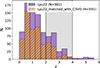 |
Fig. 1. Redshift distribution of all 901 AGNs in the Lyu et al. (2022) catalog (purple histogram). This large AGN dataset includes all nine categories of AGN defined in Lyu et al. (2022). Note: the categories are not mutually exclusive, i.e., a given AGN can satisfy the selection criteria for multiple categories of AGNs. The redshift values for these AGNs are sourced from the Lyu et al. (2022) catalog. We also overplotted the redshift distribution of 591 Lyu et al. (2022) AGNs that are matched with the C3VO (MUSYC) sources within a projected separation of 0.5 (orange histograms with purple lines). The redshift distribution peaks around z ∼ 0.75, and almost vanishes at z > 4. In this study, we restricted our analysis to the redshift range of 2.0 < z < 4.0 as shown by the gray shaded region between the two black dashed vertical lines. |
2.2.2. AGN Selection criteria
To probe populations of different types of AGN, Lyu et al. (2022) applied various selection criteria on the multiwavelength source catalog described above. The nine categories of AGN presented in Lyu et al. (2022) are summarized below, along with the selection criteria used for the identification of AGNs of each category. For each category, we also provided the average number of AGNs in our sample, focusing on the redshift range 2.0 < z < 4.0. These average values are taken from the mean of the fractions estimated over the 100 Monte Carlo realizations of our data (see Sect. 2.4 for a description of the Monte Carlo process):
2.2.2.1. MIR-SED:
AGNs in this category exhibit a notable excess emission in the NIR to MIR (λ ∼ 2 − 8 μm) from hot to warm dust. There are 288 MIR-SED AGNs in the Lyu et al. (2022) catalog. Lyu et al. (2022) conducted SED fitting of galaxies using the SED fitting tool Prospector (Johnson et al. 2021). They utilized the Flexible Stellar Population Synthesis (FSPS) stellar model from Prospector, along with their own (semi) empirical models of dust emission and AGN continuum emission (Lyu et al. 2017; Lyu & Rieke 2017, 2018). To identify AGN based on an SED analysis, they required for the best-fitting SED contains a significant AGN component with LAGN > 108 L⊙. For these cases, the SED fits are visually inspected to discard the cases for which the fitting solutions are degenerate with multiple peaks of the LAGN posterior as well as the cases for which the photometric constraints are too limited to determine if the AGN component exists. In cases where the classification of objects is unclear, the method involves conducting SED fitting both with and without an AGN component. If the inclusion of the AGN component results in the chi-square values being reduced by a factor of 2.5 or more, the object is then categorized as a MIR SED AGNs. For cases with LAGN > 108 L⊙ but visual inspection of borderline or marginal, they conducted an SED fitting both with and without an AGN component. Similarly to other objects, for these cases, if the inclusion of the AGN component results in the chi-square values of the data being reduced by a factor of 2.5 or more, the object is categorized as an MIR SED AGN. On average, there are ∼27 MIR-SED AGNs in our sample.
2.2.2.2. Mid-IR-COLOR:
These objects have MIR colors that are dominated by AGN warm-dust emission. They are selected using the criterion of log(S5.8/S3.6) > 0.08 and log(S8.0/S4.5) > 0.15 from Kirkpatrick et al. (2017). Lyu et al. (2022) list 104 MIR-COLOR AGNs in their catalog. Our AGN sample contains an average of ∼13 MIR-COLOR AGNs.
2.2.2.3. X-ray-lum:
These objects have an intrinsic X-ray luminosity that is higher than expected for stellar processes in galaxies. These AGNs were identified using LX, int > 1042.5 erg s−1 (Luo et al. 2017). For cases with slightly lower intrinsic X-ray luminosity cut (LX, int > 1042.0 erg s−1) if their SED fittings suggested low SFRs (≲10 M⊙ yr−1), they were determined to be AGNs (e.g., Pereira-Santaella et al. 2011; Mineo et al. 2014; Symeonidis et al. 2014; Algera et al. 2020). The observed X-ray luminosity distribution with redshift is shown for all Lyu et al. (2022) AGNs that have values of Lxobs > 0 in Figure 2. The figure also shows this distribution for such sources that are also matched to the C3VO (MUSYC) sources within a projected separation of 0.5″. Lyu et al. (2022) identified 321 AGNs satisfying their X-ray-lum criteria. On average, in our sample, there are ∼41 AGNs selected in this X-ray-lum category.
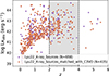 |
Fig. 2. Distribution of the observed X-ray luminosity (Lxobs) vs. redshift (z) for all 658 sources in Lyu et al. (2022) with Lxobs > 0.0 (purple filled circles). Out of them, the 435 sources that are matched to the C3VO sources within a separation of 0.5″ are highlighted (purple filled circles with orange edge colors). The redshifts for the Lyu et al. (2022) sources are from their AGN catalog, which are sourced from the 3D-HST catalog. For this study, we only focused on redshift range of 2.0 < z < 4.0 as shown by the gray shaded region between the two black dashed vertical lines. |
2.2.2.4. X2R:
These objects have an X-ray (0.5–7 keV) to radio (3 GHz) luminosity ratio higher than expected for stellar processes in a galaxy. These AGNs are identified using the criterion of LX, int[erg/s]/L3 GHz[W/Hz] > 8 × 10¹⁸. In their catalog, Lyu et al. (2022) report 588 X2R AGN. Our AGN sample consists of an average ∼51 X2R AGNs.
2.2.2.5. Radio-loud:
These objects are radio-loud AGNs with excess emission in the radio band compared with the prediction of templates of normal star-forming galaxies (SFGs). They are selected using q24, obs = log(S24 μm, obs/S1.4 GHz, obs), q24, obs < q24, temp. Here, S24 μm, obs and S1.4 GHz, obs are the observed MIPS 24 μm flux and the radio flux density at 1.4 GHz, respectively. S1.4 GHz, obs is computed by extrapolating the 3 GHz flux assuming that the radio spectrum can be described as a power law with α = −0.7. q24, obs is computed following Alberts et al. (2020). q24, obs is then compared to q24, temp, which is from the radio-IR correlations based on the Rieke et al. (2009) SFG templates at the appropriate redshifts. An object that is 0.5 dex below the midpoint of the radio–infrared relation with more than a 2σ significance is classified as an AGN. We note that as they compare radio emission with emission at 24 μm, their definition of radio-loud AGN differs from its canonical definition in the literature, where the radio-emission is compared with the optical brightness (Kellermann et al. 1989; Padovani 1993; La Franca et al. 1994). The selection criterion of Lyu et al. (2022) is very conservative, which might have resulted in many AGNs that would have satisfied the traditional radio-AGN criteria (see, e.g., Lemaux et al. 2014, among many others) being missed in the Lyu et al. (2022) AGN sample. Lyu et al. (2022) found 43 radio-loud AGNs. Our AGN sample contains, on average, four radio-loud AGNs.
2.2.2.6. Radio-slope:
Assuming a power-law spectrum (fν ∝ να) between the observed 3 GHz and 6 GHz bands, Lyu et al. (2022) calculated the radio slope of any given object. The object with a slope index α of more than –0.5 with a 2σ significance is considered to be a flat-spectrum radio source and identified as an AGN. There are 18 AGNs in the Lyu et al. (2022) catalog identified using this criteria. Our AGN sample does not contain any AGN identified using this radio-slope criteria.
2.2.2.7. Opt-spectroscopy:
This type of AGN shows optical spectra with hydrogen broad emission lines or hard line ratios usually caused by AGN-driven gas ionization. These AGNs are identified using either of the two criteria: (i) narrow-line AGNs presented in Santini et al. (2009) identified using Baldwin, Phillips & Terlevich (BPT) (Baldwin et al. 1981) criteria or (ii) broadline AGN presented in Silverman et al. (2010) identified based on FWHM(Hα) > 1000–2000 km/s. Lyu et al. (2022) selected 22 radio-detected and 26 radio-undetected AGNs by cross-matching these AGNs with the 3D-HST sample. Hence, they reported a total of 48 AGNs selected based on opt-spectroscopy-based criteria. Our AGN sample contains, on average, nine AGNs selected from this category.
2.2.2.8. Opt-SED:
These objects are classified as an optical SED AGN as they have LAGN > 108 L⊙ for their best-fit SED as well as a significant UV/optical excess above the stellar component which is attributed to an optically blue AGN component. Lyu et al. (2022) reported 99 opt-SED AGNs in their catalog. On average, our AGN sample contains ∼3 opt-SED AGNs.
2.2.2.9. Variable AGN:
These objects exhibit a significant photometric variation at any wavelength within either the X-ray or optical wavebands. They are identified based on their higher median absolute deviation (e.g., Pouliasis et al. 2019). Lyu et al. (2022) included variable AGN identified in optical by Pouliasis et al. (2019) and in the X-ray by Young et al. (2012) and Ding et al. (2018). There are 111 variable AGNs in the Lyu et al. (2022) catalog and our AGN sample contains, on average, seven variable AGNs.
All 901 AGNs reported in Lyu et al. (2022) are unique systems, that is, they each satisfy at least one of the nine AGN selection criteria. We note that the AGN categories are not mutually exclusive, namely, a given system can be identified as an AGN in multiple categories. In their Figure 1, Lyu et al. (2022) shows the overlap of sources in various AGN categories. While our AGN selection does not explicitly exclude obscured AGNs (e.g., type II AGNs), we acknowledge that the completeness of our sample for such sources is limited to those exhibiting strong emission in non-optical bands. Since obscured AGNs often emit strongly in the X-ray or IR, many can still be identified through selection criteria in those bands (e.g., Zakamska et al. 2003; Yan et al. 2011; Hickox et al. 2009; Donley et al. 2012), and such sources are present in our sample. However, the identification of optically selected type II AGNs using narrow emission lines is not feasible across our full redshift range, primarily due to varying spectral coverage and depth. Therefore, while some type II AGNs are captured via our multiwavelength selection, our sample is likely biased toward more luminous and less obscured sources. We note this as a limitation to consider when interpreting AGN fractions across environments in this study.
2.2.3. AGN matching
To identify AGNs within our galaxy sample, we cross-matched the 3D HST coordinates of optical/NIR AGNs counterparts provided in the Lyu et al. (2022) catalog with the coordinates of galaxies in our galaxy sample, using a nearest-neighbor matching radius of 0.5″. For only one case multiple matches were found, and we selected the match that had the most similar redshifts in the C3VO and the Lyu et al. (2022) catalogs. We note that we also checked for a presence of a bulk astrometric offset between our galaxy coordinates from Cardamone et al. (2010) and the coordinates of the optical/NIR counterparts of Lyu et al. (2022) AGNs selected from the 3D-HST catalog and found no appreciable offset. Out of 901 AGNs reported in the Lyu et al. (2022) catalog, 591 AGNs are matched to C3VO (MUSYC) sources within a projected separation of 0.5″. The redshift distribution of all Lyu et al. (2022) AGNs and the ones that are matched with C3VO sources is shown in Figure 1. For approximately 25% of sources that do not have a match in C3VO, the lack of matching seems to be caused by strong deblending of C3VO sources into multiple sources in the 3D-HST catalog. Most of the remaining sources are missed due to the difference in the depth of observations between the two catalogs, the C3VO catalog adopted here being shallower between the two. In spite of its shallowness, we used the C3VO catalog instead of the deeper catalogs, which are only available for parts of the ECDFS field, to prioritize uniformity across the ECDFS field in our VMC mapping process.
2.3. Estimation of stellar mass using spectral energy distribution fitting
We estimated the properties of galaxies, such as their stellar mass, by utilizing the SED fitting code LePhare (Arnouts et al. 1999; Ilbert et al. 2006) for the photometry described above included in the Cardamone et al. (2010) catalog. For the SED fitting process, we fixed the redshift of the galaxy to its spectroscopic redshift zspec (if available) or photometric redshift zphot. The methodology used here is the same as that used in Le Fèvre et al. (2015), Tasca et al. (2015), Lemaux et al. (2022). Briefly, we fitted a range of Bruzual & Charlot (2003) synthetic stellar population models to the observed photometry (magnitudes) in different wavebands. These population models were created based on a Chabrier (2003) initial mass function (IMF), a range of dust contents and stellar-phase metallicities, and exponentially declining and delayed SFHs. The output of the SED fitting process in LePhare includes the marginalized probability distribution function (PDF) of various physical parameters, such as stellar mass. Stellar masses of galaxies were used only as a test for examining the impact of a stellar mass-limited sample on AGN enhancement, and were not used for the final AGN enhancement results presented in this paper.
2.4. Measurement of local overdensity using VMC mapping
We used a metric of local overdensity σδ to measure the environment of galaxies. We calculated this metric using a modified version of the Voronoi tessellation used in many studies (e.g., Lemaux et al. 2017, 2018; Tomczak et al. 2017). The version of the VMC mapping used for this study is described in detail in Lemaux et al. (2022). This method partitions an area into discrete regions called Voronoi cells. A Voronoi cell consists of all points in the area that are closer to one particular predefined point (galaxy) than to any other predefined points. The edges between these cells are at the same distance from the nearest two or more galaxies, ensuring that each cell is uniquely associated with the closest galaxy. Furthermore, the sizes of these cells vary based on the proximity of galaxies to one another. This variation in cell size effectively captures the variability in galaxy distribution and serves as a robust indicator of local galaxy density.
This method cannot be directly applied to the redshift dimension due to uncertainties caused by peculiar velocities in spectroscopically confirmed galaxies and relatively large uncertainties in the photometric redshifts. These uncertainties complicate the spatial analysis as they affect the precise location of galaxies in the redshift space. To mitigate these complications, we divided the volume into redshift slices, and apply the VMC method in the projected space of each redshift slice. The redshift slice widths are chosen based on the approximate sizes of protoclusters in simulations (Chiang et al. 2013; Muldrew et al. 2015; Contini et al. 2016; Lim et al. 2024), with an additional margin to account for peculiar motion.
Our approach incorporates both spectroscopic and photometric redshifts, adjusting for their respective uncertainties to determine the most suitable redshifts for various Monte Carlo iterations as described in detail in Lemaux et al. (2022). We note that we did not use the spectroscopic redshifts of galaxies as absolute truth; instead, we treated them in a probabilistic manner. Similarly, for the probabilistic consideration of the photometric redshifts, we used the median redshift and 16th and 84th percentile of the redshift PDF. Our treatment of the redshifts of galaxies based on Monte Carlo technique is identical to the technique used in Shah et al. (2024), Forrest et al. (2023), Staab et al. (2024) and described in detail in the appendix of Lemaux et al. (2022). In brief, we generated a suite of 100 Monte Carlo (MC) realizations of zgal. If the galaxy does not have a spectroscopic redshift, then zgal was chosen from an asymmetric Gaussian distribution of zphot based on the median value of the photometric redshift and its 1σ errors (16th and 84th percentile of the photometric redshift PDF). If the galaxy had a spectroscopic redshift, then the selection of zspec as zgal is based on reliability, namely, the quality flag of the zspec. Galaxies with secure spectroscopic redshift (reliability ∼99.3%) quality flag of 3 or 4 had their zspec selected as zgal for ∼99.3% of all 100 MC iterations. For the rest of the iterations, their zgal was drawn from their asymmetric Gaussian distribution of zphot. Similarly, for galaxies with the spectroscopic redshift (reliability ∼70%) quality flag of 2 or 9, for ∼70% iterations, zspec was used as zgal, and for the rest of the iterations, zgal was drawn from their asymmetric Gaussian distribution of zphot. All 100 MC iterations were utilized for the AGN fraction analysis, as described in Section 3.
The VMC technique is capable of yielding measurements of galaxy overdensity (δgal) and the statistical significance of these overdensities (σδ) across a three-dimensional grid aligned with the right ascension (RA), declination (DEC), and redshift (z) axes. For additional information on the computation of these metrics, we refer to Forrest et al. (2023) and Shah et al. (2024). The overdensity values assigned to any given galaxy would correspond to the σδ of the nearest Voronoi cell to the galaxy’s coordinates and its zgal. For 120,525 cases (i.e., average ∼1205 objects per MC iteration), where zgal is between 2.0 < zgal < 4.0, the redshift vs. σδ distribution over all 100 MC iterations is shown in Figure 3. As the figure shows, we divided the galaxy sample in 3 different overdensity bins of (i) σδ < 2 (coeval field), (ii) 2 < σδ < 5 (intermediate overdensity), (iii) σδ > 5 (highest overdensity peaks) for our analysis (see details in Sect. 3).
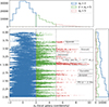 |
Fig. 3. Distribution of redshift vs. σδ (local galaxy overdensity) for 120 525 objects with 2.0 < zgal < 4.0 across the 100 Monte Carlo realizations. The number of objects is approximately 100 times higher than the true number of galaxies, averaging around 1205 objects per Monte Carlo iteration. The scatter points represent galaxies with their MC realization-specific local overdensity (σδ): coeval field (σδ < 2.0) (blue points), intermediate overdensities (2.0 < σδ < 5.0) (green points), and highly overdense peaks (σδ > 5.0) (red points). The histograms on top show the σδ distribution and the histograms on right show the redshift (zgal) for the three σδ bins: σδ < 2.0 (solid blue line), 2.0 < σδ < 5.0 (dashed green line), and σδ > 5.0 (dotted red line). The dashed gray lines show the division of the local overdensity in the three different bins used in our analyses. We also write the given names (gray text) of all five spectroscopically confirmed massive (Mtot ≥ 1014.8 M⊙) protostructures that are at z < 4 as presented in Shah et al. (2024) along with their redshift extent (horizontal dashed lines above and below the protostructure names). Furthermore, we also show the redshift of the most massive (Mtot = 1014.7 M⊙) protostructure in 2.0 < z < 4.0, which is located at z ∼ 2.45, and spread over 2.40 < z < 2.48. The broad horizontal stripe at z ∼ 3.05 consists of four protostructures, each less massive than those discussed in Shah et al. (2024). Likewise, the stripe at z ∼ 2.05 corresponds to a single protostructure with lower mass than the z ∼ 2.45 structure reported in this paper. Signs of these additional structures are visible in the figure above, but are not discussed in detail in Shah et al. (2024) or in the present paper due to their lower masses. |
Using the VMC maps, a protostructure was defined as a contiguous envelope of VMC cells, where each cell has an overdensity of more than 2.5 times the RMS of the density distribution in a given slice as measured by fifth-order polynomial to σ vs. z. In Shah et al. (2024), we presented six spectrosocopically confirmed massive (Mtot ≥ 1014.8 M⊙) protostructures at 2.5 < z < 4.5. In this study, we excluded the redshift range of 4 < z < 4.5 due to limiting depth of multiwavelength observations significantly affecting the number of AGNs (see Figure 1 and Figure 2) in this redshift range. Therefore while the first five protostructures Drishti (Mtot ∼ 1014.9 M⊙, z ∼ 2.67), Surabhi (Mtot ∼ 1014.8 M⊙, z ∼ 2.80), Shrawan (Mtot ∼ 1015.1 M⊙, z ∼ 3.3), Smruti (Mtot ∼ 1015.1 M⊙, z ∼ 3.47), and Sparsh (Mtot ∼ 1014.8 M⊙, z ∼ 3.70) from Shah et al. (2024) are included in this study, the highest redshift structure Ruchi (Mtot ∼ 1015.4 M⊙) at z ∼ 4.14 is not included. The redshift of these five massive spectroscopically confirmed protostructures is also showed in Figure 3.
Furthermore, for this study, we extended the lower bound of the redshift to z = 2, selecting the redshift range of 2 < z < 4 for our analysis. Below this redshift bound (z < 2), VUDS and C3VO do not effectively target galaxies. By extending the lower redshift bound from z = 2.5 used in Shah et al. (2024) to z = 2.0 in this study, we were able to considerably increase the galaxy sample and the corresponding AGN sample.
The redshift range of 2 < z < 2.5 was not considered in Shah et al. (2024) because that study concentrated on six of the most massive protostructures within the redshift range 2.5 < z < 4.5. Thus, it is no coincidence that these six protostructures are the most massive protostructures in the extended range of 2.0 < z < 4.5, surpassing all protostructures in the 2 < z < 2.5 range in terms of mass. We show the total mass distribution of all large structures (Mtot > 1012 M⊙) in the three redshift bins of 2.0 < z < 2.5, 2.5 < z < 3.0, and 3.0 < z < 4.0 in Figure 4. These structures are identified based on a search consistent with the process described in Shah et al. (2024). There are considerably more highly massive (Mtot > 1014 M⊙) structures at higher redshift compared to in the lowest redshift bin. We present the most massive structure in the redshift range of 2.0 < z < 2.5 below.
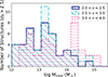 |
Fig. 4. Total mass distribution of massive (Mtot > 1012 M⊙) structures (contiguous envelope consisting of voxels with σδ > 2.5) in three different redshift bins: 2.0 < z < 2.5 (navy solid line), 2.5 < z < 3.0 (turquoise dashed line), and 3.0 < z < 4.0 (pink dotted line). |
The most massive protostructure in the redshift range of 2.0 < z < 2.5 is at z ∼ 2.45, which is spread over 2.40 < z < 2.48. The 3D distribution of the local overdensity distribution in this protostructure along with its two massive (Mtot > 1013 M⊙) overdensity peaks is shown in Figure 5. It has a total mass of Mtot = 1014.7 M⊙ and volume of 7387 cMpc3.
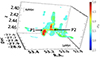 |
Fig. 5. 3D distribution of local overdensity in ECDFS, highlighting the most massive protostructure (Mtot = 1014.7 M⊙) at z ∼ 2.45, spread over 2.40 < z < 2.48. The protostructure encapsulates two massive (Mtot > 1013.25 M⊙) overdensity peaks (σδ > 5.0) shown as P1 and P2. |
To summarize the galaxy sample selection and its property estimation process described in this entire section, the final galaxy sample consists of all 100 MC iterations as described in Sect. 2.4. For each galaxy in a given MC iteration, we estimate the stellar mass using SED fitting for its redshift zgal, and the overdensity σδ value using the VMC maps and the location of galaxy (RA, Dec, zgal). Consequently, the redshift, zgal, and, thus, the stellar mass and σδ of a given galaxy may vary across different MC iterations. We only selected galaxies with IRAC1 or IRAC2 magnitudes brighter than 24.8 and 2 < zgal < 4. Using these criteria, we generated a sample of 5 514 700 objects (i.e., × 100 Monte Carlo iterations for 55 147 unique objects). Out of these, there are 120 525 cases where 2 < zgal < 4 over all 100 iterations. The zgal and σδ distribution of the 120 525 cases (i.e., average ∼1205 objects per MC iteration) are shown in Figure 3.
3. AGN fraction analysis
We defined the AGN fraction as the ratio of the number of AGN to the total number of galaxies. We calculated the AGN fraction in each of the 100 MC iterations and use the median AGN fraction value of all iterations as the final AGN fraction. For the errors on the AGN fraction, we used the 16th and 84th percentiles of the AGN fraction in all MC iterations, added in quadrature with the error on the number of AGN fraction values computed by assuming binomial statistics (Cameron 2011).
3.1. Enhancement in AGN fraction with local environment
For our entire sample (2.0 < z < 4.0), we show the change in the AGN fraction (in %) of galaxies with local overdensity (σδ) in Figure 6. As the AGN fraction increases from 1.9 % for galaxies in the coeval field, namely, σδ < 2 to 10.9
 % for galaxies in highly overdense peaks, i.e., σδ > 5, which is a clear trend of an increasing AGN fraction with the increasing overdensity of galaxies. This difference in AGN fraction is at ∼3.9σ level.
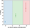 |
Fig. 6. Variations in the AGN fraction (in %) with local overdensity (σδ) for all different types of AGNs combined at 2 < z < 4. The σδ is divided into three different bins – (i) σδ < 2.0 (blue): coeval field, (ii) 2.0 < σδ < 5.0 (green): intermediate overdensity, (iii) σδ > 5 (red): highest overdensity peaks. The figure shows a clear trend of an increasing AGN fraction with the increasing local overdensities of galaxies. |
To check the sensitivity of our results to the stellar mass limit of galaxies in our redshift range, we conducted a test to see if the AGN fraction results vary when using a redshift-based 80% stellar-mass completeness limited galaxy sample instead of our entire sample. The trend described above remains unchanged and we do not see a significant difference in the results for this stellar-mass limited sample as shown in Appendix A.
3.1.1. AGN fraction of various AGN types in different environments
We show the values of AGN fraction (in %) corresponding to the different types of AGN in these local overdensity bins in Figure 7. There are five categories of AGN that have on average, more than eight AGNs across all MC iterations. These categories are: MIR, MIR-color, X-ray-lum, X2R, and opt-sp. We find that for all of these five categories, there is a clear trend of an increasing AGN fraction with the increasing overdensity, as shown in the figure. Out of all of these categories, we see the highest AGN fraction for the X2R category compared to the rest of the four categories in all environment overdensity bins. For the X2R category, the AGN fraction increases from 1.0 % to 8.2
 (∼3.5σ level) as the local ovendensity increases from σδ < 2.0 to σδ > 5.0.
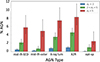 |
Fig. 7. AGN fraction (in %) for the different types of AGN in different overdensity bins: coeval field (blue) intermediate overdensity (green), and highest overdensity peaks (red). Here, we only show the five categories (MIR-SED, MIR-color, X-ray-lum, X2R, and opt-sp) for which, on average, there are more than eight AGNs across all 100 MC iterations. Note: the categories are not mutually exclusive and an AGN may meet the criteria for more than one category. See Figure 11 in Lyu et al. (2022) for the overlap of sources in different AGN categories. The asymmetric 1σ errors on these AGN fractions are shown. For all categories, there is a clear trend of higher AGN fraction for galaxies in denser environments. |
3.1.2. AGN fraction as a function of stellar mass and environment
To study the change in the AGN fraction with environment for different stellar masses of the AGN host galaxies, we divided our entire galaxy sample into two different stellar mass bins: M* > 1010.2 M⊙ and M* ≤ 1010.2 M⊙. The median stellar mass in these two bins differ approximately by an order of magnitude (∼109.5 M⊙ vs. ∼1010.4 M⊙); however, the median stellar mass in different environments is similar (with a difference of ≤0.1 dex) within each of these two mass bins. The change in the AGN fraction with the local overdensity in the subsamples of the two mass bins is shown in Figure 8. For the higher stellar mass bin (M* > 1010.2 M⊙), the AGN fraction increases from 10.3 % for σδ < 2.0 to 42.1
 % (a ∼2.9σ increment) for σδ < 5.0. Similarly, for the lower stellar mass bin (M* < 1010.2 M⊙), the AGN fraction increases from 1.1
 % for σδ < 2.0 to 4.0
 % (a ∼2.3σ increment) for σδ < 5.0. Notably, at the same local environment for all environmental bins, galaxies in the higher stellar mass bin have an AGN fraction that is ∼10× higher than their counterparts in the lower stellar mass bins in all three environment bins. This increment (∼10×) in the AGN fraction with a 10× increase in stellar mass in a given local overdensity environment, is higher compared to the increment (∼4×) in the AGN fraction with the change in the local overdensity of environment (σδ < 2.0 to σδ > 5.0) at a given stellar mass of the AGN host galaxies.
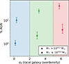 |
Fig. 8. Variations in the AGN fraction (in %) with local overdensity (σδ) for all different types of AGN combined at 2 < z < 4 in two different mass bins divided at M* = 1010.2 M⊙. The σδ bins are the same as in Figure 6. The diamond points correspond to galaxies with M* > 1010.2 M⊙ and star points correspond to galaxies with M* < 1010.2 M⊙. The figure shows a clear trend of an increasing AGN fraction with the increasing local overdensities of galaxies in both stellar mass bins. |
3.1.3. AGN fraction as a function of redshift and environment
We further divided our entire sample in three different redshift bins of 2.0 < z < 2.5, 2.5 < z < 3.0, and 3.0 < z < 4.0. We show the AGN fraction for different environments in these three redshift bins in Figure 9. For 3.0 < z < 4.0, the AGN fraction increases from 1.1 % for σδ < 2.0 to 8.7
 % (∼3.2σ level) for σδ > 5.0. Except for the highest overdensity bin for the lowest redshift bin (σδ > 5 and 2.0 < z < 2.5), all other points show a clear and continuous trend of an increasing AGN fraction with the increasing overdensity in all three redshift bins. In the intermediate overdensity bin, the AGN fraction of galaxies in the highest redshift bin is slightly lower (1.5–2.5σ) than in the other two redshift bins. Meanwhile, the AGN fraction remains roughly consistent across redshift bins in the low and high overdensity bins. This trend is influenced by factors such as variations in the completeness of Lx, obs (Figure 2) and other multiwavelength observations used for AGN identification. We also note that the intrinsic AGN fraction for different types can also vary significantly with redshift. So our results at different redshifts are affected by both of these factors. However, even considering these variations, we still see higher AGN fractions in denser local environments compared to the coeval fields at all redshifts.
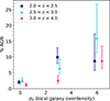 |
Fig. 9. Variations in the AGN fraction (in %) with local overdensity for all different types of AGN combined in three different redshift bins of 2.0 < z < 2.5 (navy squares), 2.5 < z < 3.0 (cyan triangles), and 3.0 < z < 4.0 (pink pentagons). Almost all points show a higher AGN fraction in denser environments at all redshifts. |
3.2. Enhancement in AGN fraction with global environment
In addition to local environment metrics, considering the global environment offers a complementary view of any potentially environment-related factors influencing AGN activity. The global environment includes large-scale structures such as clusters, filaments, and voids, which can significantly affect galaxy properties and evolution. While local overdensity metrics capturing the immediate surroundings of a galaxy, global overdensity metrics provide insights into its larger scale environment. The global environment can reveal the influence of large-scale gravitational potential wells and other dynamical processes that might not be apparent from local densities alone. This is particularly important for understanding the role of massive protostructures in galaxy evolution. Furthermore, local and global environments can influence galaxies in different ways. While local density likely correlates with immediate processes like galaxy mergers and interactions, the global environment can impact broader phenomena such as gas accretion, stripping, and the infall of galaxies into larger structures. By combining both local and global measures, we can identify if certain trends in AGN activity are consistent across different scales or if they exhibit scale-dependent behavior. This helps in understanding the multiscale nature of environmental effects on galaxies.
To study the variation in the AGN fraction of galaxies with their global environment, we computed an environment metric based on the location of galaxies with regards to its closest massive (Mtot > 1012.8 M⊙) 5σδ peak. We note that such peaks are typically embedded in protostructures with mass of more than 1014 M⊙, namely, through these systems, we are probing cores of protoclusters (See Appendix B). We defined this metric by Rproj, norm = Rproj/Reff. Here, Rproj is the projected distance of the galaxy from its closest 5σδ peak and Reff is the effective radius (Reff = (Rx+Ry)/2) of the corresponding 5σδ peak, where Rx and Ry are the effective radii of a peak along the RA and Dec directions, respectively. Mathematically, they are analogous to the standard deviation of the peak in each transverse coordinate, weighted by the local overdensity.
For each galaxy in any MC iteration, we first identified all 5σδ peaks in the ECDFS field where the galaxy’s redshift falls within the redshift range of the peak, allowing for a buffer of ±0.05 (i.e., zext ± 0.05). Additionally, we ensured that the galaxy is within a projected separation (Rproj) of less than 10 cMpc from the peak. Then we selected the peak for which Rproj, norm value is the lowest for the given galaxy in order to study the relation of AGN fraction of galaxies with their global environment. The galaxies that have an associated peak identified using this method are considered to be in dense environments. The galaxies in 2 < z < 4 that (i) do not have an associated peak (i.e., zgal outside zext ± 0.05 for all peaks) or (ii) Rproj of more than 10 cMpc – make a coeval field sample used for a comparison. For this analysis, we only considered massive (Mtot > 1012.8 M⊙) 5σ peaks as they are likely associated with massive protostructures, providing probes for denser large-scale global environments.
The AGN fraction for galaxies with an associated peak as well as galaxies in this coeval field sample is shown as a function of Rproj, norm in Figure 10. For the galaxies closest to the overdense peaks (Rproj, norm < 1.0), namely, the highest global overdensity, we observe a higher AGN fraction of 5.0 % (a ∼2.0σ increment), compared to AGN fraction (2.7
 %) of the coeval field galaxies. Hence, similar to the local environment result, we see a higher AGN activity for galaxies in a denser environment as compared to coeval field galaxies. Our results are not sensitive to the threshold (Rproj, norm < 1) used for the lowest bin, the mass-threshold (Mtot > 1012.8 M⊙), or the buffer (zext ± 0.05) around the 5σ peaks. We note that the value of the AGN fraction increases further (though not statistically significantly) for the lowest Rproj, norm bin as we decrease the upper limit from Rproj, norm = 1.
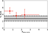 |
Fig. 10. AGN fraction (in %) as a function of global environment Rproj, norm = Rproj/Reff (red points), where Rproj is the projected distance of the galaxy from its nearest 5σδ peak and Reff is the effective radius of the corresponding 5σδ peak. The solid black line is the AGN fraction value for the corresponding coeval field, with its 1σ errors shown using dashed black lines. |
The AGN fraction of 5.0 % for the highest global overdensity (Rproj, norm < 1.0) is lower compared to the AGN fraction of 10.9
 % for the highest local overdensity (σδ > 5.0) bin shown in Figure 6. Furthermore, the AGN fraction (2.7
 %) of the coeval field defined based on global environment as described above, is slightly higher (∼1σ level) compared to the AGN fraction (1.9
 %) corresponding to the coeval field defined based on local overdensity (σδ < 2.0). In other words, the increment in the AGN fraction with changes in local overdensity of galaxies is higher compared to the changes in their global overdensities. Part of this difference is caused by the change in the overdense galaxy sample and coeval field sample selected based on global overdensity compared to local overdensity. As we adopted a redshift cylinder around the peaks to match galaxies with peaks for the global environment measure, galaxies that have a lower local density can end up having higher global overdensity. The resultant may lower the dilution of the contrast in AGN fraction with overdensity, lowering the AGN fraction for the highest global density sample. Similarly, some galaxies that resid in highly locally overdense regions may not live in a globally rich environment. Thus, while global environment provides a complementary view to local environment, the considerate uncertainties associated with measuring and characterizing the latter prevents us from drawing strong conclusions.
4. Discussion
To study the role of the environment on AGN activity in galaxies at high redshift, we conducted an analysis of the AGN fraction across a range of environments–from coeval fields to highly dense protostructure peaks at 2.0 < z < 4.0. In this section, we discuss our results of AGN activity across local and global environments, their comparison with local and high redshift studies, and implications of such results for AGN-triggering processes at different redshifts. We also discuss our results for the stellar mass dependence of the AGN-environment relation and their comparison with the literature. Finally we discuss the implications of our results in the broader context of the evolving AGN-environment relation across cosmic time.
4.1. AGN activity across local environments
The environment of galaxies can be characterized over different spatial scales, that is, the local environment (small-scale, e.g., typical galaxy separations scales) and global environment (large-scale, e.g, galaxy clusters or protoclusters scales). To probe the local environments of galaxies, we used a local-overdensity measure (σδ), which was calculated using the VMC method described in Section 2.4. We then studied the variation in AGN fraction for galaxies residing in a range of local environments from the coeval field (σδ < 2.0) to highly overdense regions (σδ > 5.0) at 2 < z < 4. A key finding from our study was a clear trend of increasing AGN fraction with higher local galaxy overdensity at 2 < z < 4 for the combined sample, including all nine AGN types (see Figure 6). We observed a ∼5× increase in AGN fraction, with a significance of ∼3.9σ, from the coeval field (σδ < 2.0) to highly overdense regions (σδ > 5.0). We also examined this relation separately for different AGN types, specifically, for the five AGN types with an average of more than eight AGN per Monte Carlo iteration. These five types are MIR SED, MIR color, X-ray luminosity, X-ray-to-radio luminosity ratio, and optical spectroscopy. For all five AGN types, we saw the above-mentioned trend of increased AGN fraction in galaxies with higher local overdensities (see Figure 7). Regions of higher local overdensity, as defined in our study, were more likely to host processes like galaxy interactions and mergers. Therefore, our findings suggest a strong connection between these processes and elevated AGN activity at these redshifts.
The relationship between AGN incidence and the local environment of galaxies, observed in our study at 2 < z < 4, is similar to that seen at z ∼ 0, where numerous studies have reported significant AGN enhancements in interacting or merging galaxies compared to their isolated counterparts (e.g., Sanders et al. 1988; Alonso et al. 2007; Ellison et al. 2011; Satyapal et al. 2014; Weston et al. 2017; Goulding et al. 2018; Ellison et al. 2019, 2025; Comerford et al. 2024; Cezar et al. 2024) as well as at lower redshifts (z ≲ 1) (e.g., Silverman et al. 2011; Lackner et al. 2014; La Marca et al. 2024).
At intermediate redshifts and on smaller scales (i.e., in spectroscopic galaxy pairs at 0.5 < z < 3.0), Shah et al. (2020) found no significant enhancement in X-ray AGN or IR-AGN fractions relative to a stellar mass-, redshift-, and environment-matched control sample of isolated galaxies. As discussed in Fensch et al. (2017), Shah et al. (2020), and Shah et al. (2024), despite the larger gas fractions of galaxies at these intermediate redshifts compared to the local Universe, extreme gas conditions such as elevated turbulence and temperature, as well as other physical processes appear to suppress the nuclear inflow of gas that would otherwise trigger AGN during interactions and mergers.
In contrast, our study shows that at even higher redshifts (2 < z < 4), the role of the local environment-likely driven by galaxy interactions and mergers is reversed, as we observe a higher AGN fraction in denser local environments. Several factors may contribute to this observed reversal, including the increased gas supply in high-redshift galaxies (e.g., Gowardhan et al. 2019), higher merger rates (e.g., Ferreira et al. 2020), and differences in galaxy properties such as stellar mass (e.g., Ownsworth et al. 2014) and morphology (e.g., Kartaltepe et al. 2023) at these epochs. For example, the merger rate of galaxies is more than twice as high in the proto-supercluster Hyperion (Giddings et al. 2025) compared to coeval field environments. Our findings show the increasingly important role of local environmental processes-especially interactions and mergers in triggering AGN activity in the early Universe.
4.2. AGN activity across global environments
To probe the large-scale (global) environment of galaxies, we used a measure (Rproj, norm) based on the separation of galaxies from their corresponding closest massive peak, normalized by the effective radius of the peak as described in Section 3.2. We then studied the change in the AGN fraction over a large range (0–5) of Rproj, norm. Here, Rproj, norm < 1 denotes galaxies located inside their corresponding peak, while Rproj, norm > 1 indicates galaxies located outside their corresponding peak. Our results presented in Figure 10, show tentative signs (∼2σ) of an increasing AGN fraction with a decreasing Rproj, norm, namely, a decreasing normalized distance from highly overdense (σδ > 5) peaks. Therefore, this result also suggests higher AGN fraction in galaxies residing in denser global environments.
This finding is a contrast of the results of studies in local Universe showing significant decrease in the fraction of (X-ray) AGNs with a decreasing cluster-centric radius, going from r500 to central regions of clusters (e.g., Ehlert et al. 2013; Pentericci et al. 2013; Koulouridis et al. 2024). Similarly, our results vary compared to studies showing lower AGN fractions of luminous AGN in cluster galaxies compared to coeval field galaxies (Kauffmann et al. 2004; Popesso & Biviano 2006). The relationship between the incidence of AGN and environment at 2 < z < 4 also seems to contrast with results at z ∼ 1, such as those presented by Rumbaugh et al. (2017) at 0.65 < z < 1.28, which showed an absence of a strong relation between AGN activity and location within the large-scale structures (LSSs) in the ORELSE survey (Lubin et al. 2009). Additionally, (Martini et al. 2013) showed similar X-ray and MIR-selected AGN fractions in cluster galaxies and field galaxies at 1 < z < 1.5.
Therefore, similarly to the redshift-based change in the impact of the local environment on AGN activity, our results based on the global environment, along with their comparison with results at low redshift, also suggest a reversal of the AGN-environment relation at high redshift. This reversal might be occurring before z ∼ 2.0 as our results are consistent with studies based on samples of clusters (Bufanda et al. 2017), as well as studies based on individual protoclusters, such as Krishnan et al. (2017) (X-ray AGNs; z ∼ 1.7), Tozzi et al. (2022) (X-ray AGNs; z ∼ 2.156), Polletta et al. (2021) (X-ray AGNs; z ∼ 2.16), Digby-North et al. (2010) (AGN identification using emission-lines in optical/NIR spectra; z ∼ 2.2), and Monson et al. (2023) (X-ray AGNs; z ∼ 3.09), all of which show a higher AGN fraction in protocluster galaxies as compared to field galaxies.
Additionally, our X-ray-luminosity AGN fraction values in the intermediate and highly overdense environments at 2 < z < 4 are consistent with the X-ray AGN fraction in individual clusters reported by Digby-North et al. (2010) (z∼2.2) and Lehmer et al. (2009) (z ∼ 3.09). The enhancement of ∼2.5× at 3.0 < z < 4.0 in the intermediate overdensity bin compared to the field, observed in our sample, is within the error bars of the enhancement seen in individual protoclusters at z ∼ 3.09 reported by Lehmer et al. (2009) (Lyman break galaxies, X-ray AGN sample). While our findings may appear to contrast with those of Macuga et al. (2019), who did not find a relation between environment and X-ray AGN fraction in a z ∼ 2.53 protocluster, we recall here that our conclusions are based on an ensemble of protostructures. Therefore, our results do not preclude the possibility that individual protostructures might show no strong relation between environment and AGN activity. This ensemble-based approach enables us to identify average trends for a population of protostructures spanning a broad range of environments.
Another possible reason for this difference in AGN fraction in our study compared to those z > 2 studies discussed above could be the variation in the dynamical states and masses of the protoclusters in the various samples, which could result in different impacts of the environment on AGN activity in various protoclusters. As a given protocluster can show a range of impacts on AGN activity, adopting an ensemble of structures, such as the one utilized in this study, is necessary to understand the overall impact of the protocluster population on AGN activity in galaxies. Furthermore, there are also differences in the methods used to characterize protoclusters and their member galaxies between our study and these studies, which could result in variations in AGN fraction enhancement. The substantial photometric and spectroscopic data used for our galaxy sample, along with the extensive AGN sample provided by Lyu et al. (2022), have allowed us to have a large sample of galaxies and AGNs spanning a wide range of redshift and environment expanding the scope of this type of analysis.
Both of our results, based on local and global environments, show a higher AGN fraction in denser environments compared to coeval-field environments. Our analysis indicates that the enhancement in AGN fraction is more pronounced in the local environment compared to the global environment. This suggests that the processes driving the increase in AGN fraction are more effective on smaller scales rather than larger scales. As discussed earlier, smaller-scale processes like galaxy interactions or mergers could be significant factors in this enhancement. As the interaction and merger rates of galaxies (e.g., Lin et al. 2010) as well as gas reservoirs (Gururajan et al. 2025) can also vary with global environments, the global environments can also indirectly affect the AGN fraction observed in these local environments. Such large-scale changes to local conditions could then influence AGN triggering by modifying the frequency and nature of galaxy encounters in galaxy clusters, likely enhancing black hole fueling. This scenario is supported by observational studies showing that AGNs in galaxy clusters are often associated with infalling, merging, or morphologically disturbed galaxies (Haines et al. 2012; Ehlert et al. 2015; Drigga et al. 2025). These complexities, along with the dilution in AGN enhancement caused by the way global environment is measured (see Sect. 3.2), make it challenging to disentangle the impact of global environment and local environment on the AGN activity of galaxies. Despite these complexities, our findings suggest a significant redshift evolution in the influence of environment on AGN activity, highlighting the need for further investigation into the processes driving such evolution and their variation across different environment scales and cosmic epochs.
4.3. Stellar mass and redshift dependence of the AGN-environment relation
Studies show approximately an order of magnitude increment in the AGN fraction of galaxies with an increment in the host galaxy mass of an order of magnitude at lower redshifts (z ≤ 1.0) (e.g., Juneau et al. 2013; Aird & Coil 2021) and in the stellar mass range and redshift range of our study (e.g., Aird et al. 2019; Guetzoyan et al. 2025; Martínez-Marín et al. 2024). These increments are consistent with our results of approximately an order of magnitude increment in AGN fraction in the higher mass bin compared to the lower mass bin in a given environment as shown in Figure 8. We note that the cited studies are based on a single type of AGN (for example, X-ray or optical), as opposed to, the nine different AGN categories included in our study. There are also differences between our study and these studies such as the depth of multiwavelength observations, methods used to generate galaxy samples, and so on. These differences can lead to differences in the AGN fraction values observed in our study compared to these studies.
As shown in Figure 8, the increase in AGN fraction with stellar mass (at fixed local overdensity) is greater than the increase in AGN fraction with local overdensity (at fixed stellar mass). This comparison may suggest that the impact of processes related to the stellar mass-AGN connection is larger compared to that of the environment-AGN connection. Furthermore, we have observed approximately the same increase in AGN fraction with environment in both higher and lower stellar mass bins (also shown in Figure 8). These similarities may indicate that the processes driving the increase in AGN activity with environment do not strongly depend on the stellar mass of the host galaxies.
To study the redshift dependence of the AGN-environment relation, we divided our sample into three redshift bins: 2.0 < z < 2.5, 2.5 < z < 3.0, and 3.0 < z < 4.0. We observed a consistent trend of increasing AGN fraction with local overdensity across all bins, except in the highest local overdensity bin (σδ > 5) at 2.5 < z < 3.0, where low-number statistics likely limit the reliability of the result. These results suggest a strong relation between AGN incidence and the local environment of galaxies throughout the redshift range of this study.
Considering our analysis of the mass and redshift dependence of the AGN-environment relation, our results suggest that while stellar mass plays a dominant role, the local environment is also significantly and consistently associated with AGN activity in galaxies. This might imply that the processes connecting galaxy environment and AGN activity were already taking place in the early universe and despite evolving galaxy and environmental conditions, they also persisted over a long time in cosmic history.
As discussed in this section, our results present a strong multi-scale connection linking AGN activity in galaxies to both internal properties of galaxies, such as stellar-mass, and their external environments on small (local) and large (global) scales. The consistent trends between AGN incidence and galaxy environment across large spatial scales, redshift ranges, and for different AGN types in our study suggest that external environmental processes play a fundamental role in triggering AGN activity of galaxies at 2 < z < 4. Furthermore, the reversal of environment-AGN connection at such high redshifts compared to the local universe indicates that these processes evolve significantly over cosmic time.
5. Summary
We present a study on the relation of the environment of galaxies with its AGN activity at 2.0 < z < 4.0. We conducted a robust analysis on the change in the AGN fraction of galaxies with the change in the local overdensity as well as global overdensity of galaxies. These overdensities were measured using a novel environment measurement technique, utilizing deep multiwavelength spectroscopic and photometric observations in the GOODS-S field. The AGNs in our sample were sourced from the multiwavelength AGN catalog over nine categories provided by Lyu et al. (2022). We summarize our findings below.
-
For our entire galaxy sample and the AGN sample at 2.0 < z < 4.0, we see a clear trend of an increasing AGN fraction with an increasing local overdensity of galaxies. The AGN fraction of galaxies increases from 1.9
 % to 10.9
 % (a ∼3.9σ increment) as the local overdensity of galaxies increase from σδ < 2.0 (coeval field) to σδ > 5.0 (highly overdense peaks). Our results exhibit a ∼3× and ∼5× increment in the AGN fraction compared to the coeval-field for an intermediate overdensity bin (2 < σδ < 5.0) and a highly overdense bin (σδ > 5.0), respectively.
 -
The trend of an increasing AGN fraction with the increasing local overdensity of galaxies is present in all five categories of AGNs (for which there are, on average, more than eight AGNs across all 100 MC iterations), including MIR-SED, MIR-color, X-ray luminosity, X-ray-to-radio (X2R) luminosity ratio, and optical-spectroscopy at 2.0 < z < 4.0. We note that these categories are not mutually exclusive, namely, a given system can be identified as an AGN for more than one AGN categories. The highest AGN fraction is 8.2
 for σδ > 5 for X2R AGN category, which is ∼3.5σ higher than that for the coeval field σδ < 2 galaxies (1.0
 ).
). -
We divided our sample into two stellar mass bins: M* > 1010.2 M⊙ and M* ≤ 1010.2 M⊙. We observed a clear trend of higher (∼4×) AGN fractions in denser local overdensity environments in both stellar mass bins. For a given environment, the AGN fractions of the galaxies in the higher stellar mass bins are ∼10× higher compared to the galaxies in the lower stellar mass bins in all three environment bins.
-
We split the sample in three different redshift bins: 2.0 < z < 2.5, 2.5 < z < 3.0, and 3.0 < z < 4.0. The results for all three redshift bins show the trend of increasing AGN fraction with increasing local overdensity of galaxies, with an exception of σδ > 5 bin for 2.0 < z < 2.5, which is likely affected by low-number statistics. For 3.0 < z < 4.0, the AGN fraction increases from 1.1
 for σδ < 2.0 to 8.7
 (a ∼3.2σ increment) for σδ > 5.0.
 -
For global environment measure, Rproj, norm, we see a higher AGN fraction (5.0
 %) (∼2.0σ higher) for galaxies in denser global environment (Rproj, norm < 1.0) compared the AGN fraction (2.7
 %) of the corresponding coeval field galaxies.
Our results, as compared to cluster studies of the low- and intermediate-redshift Universe, suggest a reversal in the role of environment in AGN activity. Specifically, at high redshifts of 2.0 < z < 4.0, galaxies in denser environments exhibit a substantially higher AGN fraction compared to their coeval field counterparts, in contrast to the behavior seen in local clusters. This enhancement in AGN fraction in denser environments at high redshift could be caused by factors such as increased gas supply, higher merger rates of galaxies, and differences in the properties of galaxies or environments. Such a prevalence of AGN activity in these denser environments could result in increase AGN-feedback processes (e.g., AGN-driven outflows) expelling or heating gas, which could lead to the quenching of star formation in galaxies (e.g., Xie et al. 2024). Our study provides a pathway to better understanding the complex interplay between the environment and AGN activity in galaxies at high redshift. It also offers valuable constraints on environment-related impacts on AGN activity for theoretical models.
We used the more agnostic term “protostructures” (instead of protoclusters) throughout the paper as we were unsure of the fate of the systems reported in this paper.
The data used in this study would be shared based on a reasonable request to the corresponding author.
Acknowledgments
We are deeply grateful to the referee for their thorough review and thoughtful feedback, which have enriched the manuscript in several important aspects. Results in this paper were partially based on observations made at Cerro Tololo Inter-American Observatory at NSF’s NOIRLab, which is managed by the Association of Universities for Research in Astronomy (AURA) under a cooperative agreement with the National Science Foundation. Supported by the international Gemini Observatory, a program of NSF NOIRLab, which is managed by the Association of Universities for Research in Astronomy (AURA) under a cooperative agreement with the U.S. National Science Foundation, on behalf of the Gemini partnership of Argentina, Brazil, Canada, Chile, the Republic of Korea, and the United States of America. Results additionally relied on observations collected at the European Organisation for Astronomical Research in the Southern Hemisphere. This work is based on observations made with the Spitzer Space Telescope, which is operated by the Jet Propulsion Laboratory, California Institute of Technology under a contract with NASA. Some of the data presented herein were obtained at Keck Observatory, which is a private 501(c)3 non-profit organization operated as a scientific partnership among the California Institute of Technology, the University of California, and the National Aeronautics and Space Administration. The Observatory was made possible by the generous financial support of the W. M. Keck Foundation. This work was supported by NASA’s Astrophysics Data Analysis Program under grant number 80NSSC21K0986. Some of the material presented in this paper is based upon work supported by the National Science Foundation under Grant No. 1908422. The authors wish to recognize and acknowledge the very significant cultural role and reverence that the summit of Maunakea has always had within the indigenous Hawaiian community. We are most fortunate to have the opportunity to conduct observations from this mountain. For the purpose of open access, the author has applied a Creative Commons Attribution (CC BY) license to any Author Accepted Manuscript version arising from this submission.
References
- Aird, J., & Coil, A. L. 2021, MNRAS, 502, 5962 [NASA ADS] [CrossRef] [Google Scholar]
- Aird, J., Coil, A. L., & Georgakakis, A. 2019, MNRAS, 484, 4360 [NASA ADS] [CrossRef] [Google Scholar]
- Alberts, S., Rujopakarn, W., Rieke, G. H., Jagannathan, P., & Nyland, K. 2020, ApJ, 901, 168 [NASA ADS] [CrossRef] [Google Scholar]
- Algera, H. S. B., van der Vlugt, D., Hodge, J. A., et al. 2020, ApJ, 903, 139 [Google Scholar]
- Alonso, M. S., Lambas, D. G., Tissera, P., & Coldwell, G. 2007, MNRAS, 375, 1017 [NASA ADS] [CrossRef] [Google Scholar]
- Antonucci, R. 1993, ARA&A, 31, 473 [Google Scholar]
- Arnold, T. J., Martini, P., Mulchaey, J. S., Berti, A., & Jeltema, T. E. 2009, ApJ, 707, 1691 [Google Scholar]
- Arnouts, S., Cristiani, S., Moscardini, L., et al. 1999, MNRAS, 310, 540 [Google Scholar]
- Baldwin, J. A., Phillips, M. M., & Terlevich, R. 1981, PASP, 93, 5 [Google Scholar]
- Balogh, M. L., Navarro, J. F., & Morris, S. L. 2000, ApJ, 540, 113 [Google Scholar]
- Barnes, J. E., & Hernquist, L. E. 1991, ApJ, 370, L65 [Google Scholar]
- Barro, G., Pérez-González, P. G., Gallego, J., et al. 2011a, ApJS, 193, 13 [NASA ADS] [CrossRef] [Google Scholar]
- Barro, G., Pérez-González, P. G., Gallego, J., et al. 2011b, ApJS, 193, 30 [Google Scholar]
- Belli, S., Park, M., Davies, R. L., et al. 2024, Nature, 630, 54 [NASA ADS] [CrossRef] [Google Scholar]
- Best, P. N. 2004, MNRAS, 351, 70 [NASA ADS] [CrossRef] [Google Scholar]
- Birkin, J. E., Weiss, A., Wardlow, J. L., et al. 2021, MNRAS, 501, 3926 [Google Scholar]
- Blecha, L., Snyder, G. F., Satyapal, S., & Ellison, S. L. 2018, MNRAS, 478, 3056 [Google Scholar]
- Bower, R. G., McCarthy, I. G., & Benson, A. J. 2008, MNRAS, 390, 1399 [NASA ADS] [Google Scholar]
- Brammer, G. B., van Dokkum, P. G., Franx, M., et al. 2012, ApJS, 200, 13 [Google Scholar]
- Bruzual, G., & Charlot, S. 2003, MNRAS, 344, 1000 [NASA ADS] [CrossRef] [Google Scholar]
- Buchner, J., Georgakakis, A., Nandra, K., et al. 2014, A&A, 564, A125 [NASA ADS] [CrossRef] [EDP Sciences] [Google Scholar]
- Bufanda, E., Hollowood, D., Jeltema, T. E., et al. 2017, MNRAS, 465, 2531 [NASA ADS] [CrossRef] [Google Scholar]
- Cameron, E. 2011, PASA, 28, 128 [Google Scholar]
- Cardamone, C. N., van Dokkum, P. G., Urry, C. M., et al. 2010, ApJS, 189, 270 [Google Scholar]
- Cezar, P. H., Pastoriza, M. G., Riffel, R., et al. 2024, A&A, 689, A312 [NASA ADS] [CrossRef] [EDP Sciences] [Google Scholar]
- Chabrier, G. 2003, PASP, 115, 763 [Google Scholar]
- Chiang, Y.-K., Overzier, R., & Gebhardt, K. 2013, ApJ, 779, 127 [Google Scholar]
- Cisternas, M., Jahnke, K., Inskip, K. J., et al. 2011, ApJ, 726, 57 [NASA ADS] [CrossRef] [Google Scholar]
- Comerford, J. M., Nevin, R., Negus, J., et al. 2024, ApJ, 963, 53 [NASA ADS] [CrossRef] [Google Scholar]
- Contini, E., De Lucia, G., Hatch, N., Borgani, S., & Kang, X. 2016, MNRAS, 456, 1924 [NASA ADS] [CrossRef] [Google Scholar]
- Dahlen, T., Mobasher, B., Faber, S. M., et al. 2013, ApJ, 775, 93 [Google Scholar]
- Damen, M., Labbé, I., van Dokkum, P. G., et al. 2011, ApJ, 727, 1 [NASA ADS] [CrossRef] [Google Scholar]
- Di Matteo, T., Springel, V., & Hernquist, L. 2005, Nature, 433, 604 [NASA ADS] [CrossRef] [Google Scholar]
- Di Matteo, P., Bournaud, F., Martig, M., et al. 2008, A&A, 492, 31 [NASA ADS] [CrossRef] [EDP Sciences] [Google Scholar]
- Digby-North, J. A., Nandra, K., Laird, E. S., et al. 2010, MNRAS, 407, 846 [NASA ADS] [CrossRef] [Google Scholar]
- Ding, N., Luo, B., Brandt, W. N., et al. 2018, ApJ, 868, 88 [NASA ADS] [CrossRef] [Google Scholar]
- Donley, J. L., Koekemoer, A. M., Brusa, M., et al. 2012, ApJ, 748, 142 [Google Scholar]
- Donley, J. L., Kartaltepe, J., Kocevski, D., et al. 2018, ApJ, 853, 63 [NASA ADS] [CrossRef] [Google Scholar]
- Dressler, A. 1980, ApJ, 236, 351 [Google Scholar]
- Drigga, E., Koulouridis, E., Pouliasis, E., et al. 2025, A&A, 697, A234 [NASA ADS] [CrossRef] [EDP Sciences] [Google Scholar]
- Dubois, Y., Peirani, S., Pichon, C., et al. 2016, MNRAS, 463, 3948 [Google Scholar]
- Edler, H. W., Roberts, I. D., Boselli, A., et al. 2024, A&A, 683, A149 [NASA ADS] [CrossRef] [EDP Sciences] [Google Scholar]
- Ehlert, S., Allen, S. W., Brandt, W. N., et al. 2013, MNRAS, 428, 3509 [NASA ADS] [CrossRef] [Google Scholar]
- Ehlert, S., Allen, S. W., Brandt, W. N., et al. 2015, MNRAS, 446, 2709 [Google Scholar]
- Ellison, S. L., Patton, D. R., Simard, L., et al. 2010, MNRAS, 407, 1514 [NASA ADS] [CrossRef] [Google Scholar]
- Ellison, S. L., Patton, D. R., Mendel, J. T., & Scudder, J. M. 2011, MNRAS, 418, 2043 [NASA ADS] [CrossRef] [Google Scholar]
- Ellison, S. L., Mendel, J. T., Patton, D. R., & Scudder, J. M. 2013, MNRAS, 435, 3627 [CrossRef] [Google Scholar]
- Ellison, S. L., Viswanathan, A., Patton, D. R., et al. 2019, MNRAS, 487, 2491 [NASA ADS] [CrossRef] [Google Scholar]
- Ellison, S., Ferreira, L., Bickley, R., et al. 2025, Open J. Astrophys., 8, 12 [Google Scholar]
- Faber, S. M., Phillips, A. C., Kibrick, R. I., et al. 2003, SPIE Conf. Ser., 4841, 1657 [Google Scholar]
- Fabian, A. C. 1999, MNRAS, 308, L39 [NASA ADS] [CrossRef] [Google Scholar]
- Fensch, J., Renaud, F., Bournaud, F., et al. 2017, MNRAS, 465, 1934 [NASA ADS] [CrossRef] [Google Scholar]
- Ferreira, L., Conselice, C. J., Duncan, K., et al. 2020, ApJ, 895, 115 [NASA ADS] [CrossRef] [Google Scholar]
- Forrest, B., Tran, K.-V. H., Broussard, A., et al. 2017, ApJ, 838, L12 [NASA ADS] [CrossRef] [Google Scholar]
- Forrest, B., Lemaux, B. C., Shah, E., et al. 2023, MNRAS, 526, L56 [NASA ADS] [CrossRef] [Google Scholar]
- Gawiser, E., van Dokkum, P. G., Herrera, D., et al. 2006, ApJS, 162, 1 [CrossRef] [Google Scholar]
- Giavalisco, M., Ferguson, H. C., Koekemoer, A. M., et al. 2004, ApJ, 600, L93 [NASA ADS] [CrossRef] [Google Scholar]
- Giddings, F., Lemaux, B. C., Forrest, B., et al. 2025, A&A, submitted [arXiv:2503.04913] [Google Scholar]
- Ginolfi, M., Maiolino, R., Nagao, T., et al. 2017, MNRAS, 468, 3468 [CrossRef] [Google Scholar]
- Goulding, A. D., Greene, J. E., Bezanson, R., et al. 2018, PASJ, 70, S37 [NASA ADS] [CrossRef] [Google Scholar]
- Gowardhan, A., Riechers, D., Pavesi, R., et al. 2019, ApJ, 875, 6 [NASA ADS] [CrossRef] [Google Scholar]
- Grogin, N. A., Kocevski, D. D., Faber, S. M., et al. 2011, ApJS, 197, 35 [NASA ADS] [CrossRef] [Google Scholar]
- Guetzoyan, P., Aird, J., Georgakakis, A., et al. 2025, MNRAS, 536, 79 [Google Scholar]
- Gururajan, G., Cucciati, O., Lemaux, B. C., et al. 2025, A&A, 698, A312 [NASA ADS] [CrossRef] [EDP Sciences] [Google Scholar]
- Haggard, D., Green, P. J., Anderson, S. F., et al. 2010, ApJ, 723, 1447 [NASA ADS] [CrossRef] [Google Scholar]
- Haines, C. P., Pereira, M. J., Sanderson, A. J. R., et al. 2012, ApJ, 754, 97 [NASA ADS] [CrossRef] [Google Scholar]
- Hamann, F., & Ferland, G. 1999, ARA&A, 37, 487 [Google Scholar]
- Hashiguchi, A., Toba, Y., Ota, N., et al. 2023, PASJ, 75, 1246 [CrossRef] [Google Scholar]
- Hickox, R. C., Jones, C., Forman, W. R., et al. 2009, ApJ, 696, 891 [Google Scholar]
- Hildebrandt, H., Erben, T., Dietrich, J. P., et al. 2006, A&A, 452, 1121 [NASA ADS] [CrossRef] [EDP Sciences] [Google Scholar]
- Hopkins, P. F., & Quataert, E. 2011, MNRAS, 415, 1027 [NASA ADS] [CrossRef] [Google Scholar]
- Hsu, L.-T., Salvato, M., Nandra, K., et al. 2014, ApJ, 796, 60 [Google Scholar]
- Ilbert, O., Arnouts, S., McCracken, H. J., et al. 2006, A&A, 457, 841 [NASA ADS] [CrossRef] [EDP Sciences] [Google Scholar]
- Johnson, B. D., Leja, J., Conroy, C., & Speagle, J. S. 2021, ApJS, 254, 22 [NASA ADS] [CrossRef] [Google Scholar]
- Juneau, S., Dickinson, M., Bournaud, F., et al. 2013, ApJ, 764, 176 [NASA ADS] [CrossRef] [Google Scholar]
- Kara, S., Plšek, T., Protušová, K., et al. 2024, MNRAS, 528, 1500 [Google Scholar]
- Kartaltepe, J. S., Rose, C., Vanderhoof, B. N., et al. 2023, ApJ, 946, L15 [NASA ADS] [CrossRef] [Google Scholar]
- Kauffmann, G., White, S. D. M., Heckman, T. M., et al. 2004, MNRAS, 353, 713 [Google Scholar]
- Kaviraj, S., Khochfar, S., Schawinski, K., et al. 2008, MNRAS, 388, 67 [Google Scholar]
- Kawakatu, N., Anabuki, N., Nagao, T., Umemura, M., & Nakagawa, T. 2006, ApJ, 637, 104 [NASA ADS] [CrossRef] [Google Scholar]
- Kellermann, K. I., Sramek, R., Schmidt, M., Shaffer, D. B., & Green, R. 1989, AJ, 98, 1195 [Google Scholar]
- Kim, D., Sheen, Y.-K., Jaffé, Y. L., et al. 2024, ApJ, 966, 124 [NASA ADS] [CrossRef] [Google Scholar]
- Kirkpatrick, A., Alberts, S., Pope, A., et al. 2017, ApJ, 849, 111 [NASA ADS] [CrossRef] [Google Scholar]
- Klesman, A. J., & Sarajedini, V. L. 2012, MNRAS, 425, 1215 [Google Scholar]
- Kocevski, D. D., Faber, S. M., Mozena, M., et al. 2012, ApJ, 744, 148 [NASA ADS] [CrossRef] [Google Scholar]
- Koekemoer, A. M., Faber, S. M., Ferguson, H. C., et al. 2011, ApJS, 197, 36 [NASA ADS] [CrossRef] [Google Scholar]
- Koulouridis, E., Plionis, M., Chavushyan, V., et al. 2013, A&A, 552, A135 [NASA ADS] [CrossRef] [EDP Sciences] [Google Scholar]
- Koulouridis, E., Ricci, M., Giles, P., et al. 2018, A&A, 620, A20 [NASA ADS] [CrossRef] [EDP Sciences] [Google Scholar]
- Koulouridis, E., Gkini, A., & Drigga, E. 2024, A&A, 684, A111 [NASA ADS] [CrossRef] [EDP Sciences] [Google Scholar]
- Kriek, M., Shapley, A. E., Reddy, N. A., et al. 2015, ApJS, 218, 15 [NASA ADS] [CrossRef] [Google Scholar]
- Krishnan, C., Hatch, N. A., Almaini, O., et al. 2017, MNRAS, 470, 2170 [NASA ADS] [CrossRef] [Google Scholar]
- La Franca, F., Gregorini, L., Cristiani, S., de Ruiter, H., & Owen, F. 1994, AJ, 108, 1548 [Google Scholar]
- La Marca, A., Margalef-Bentabol, B., Wang, L., et al. 2024, A&A, 690, A326 [NASA ADS] [CrossRef] [EDP Sciences] [Google Scholar]
- Lackner, C. N., Silverman, J. D., Salvato, M., et al. 2014, AJ, 148, 137 [NASA ADS] [CrossRef] [Google Scholar]
- Le Fèvre, O., Saisse, M., Mancini, D., et al. 2003, SPIE Conf. Ser., 4841, 1670 [Google Scholar]
- Le Fèvre, O., Vettolani, G., Paltani, S., et al. 2004, A&A, 428, 1043 [CrossRef] [EDP Sciences] [Google Scholar]
- Le Fèvre, O., Cassata, P., Cucciati, O., et al. 2013, A&A, 559, A14 [Google Scholar]
- Le Fèvre, O., Tasca, L. A. M., Cassata, P., et al. 2015, A&A, 576, A79 [Google Scholar]
- Lehmer, B. D., Brandt, W. N., Alexander, D. M., et al. 2005, ApJS, 161, 21 [NASA ADS] [CrossRef] [Google Scholar]
- Lehmer, B. D., Alexander, D. M., Geach, J. E., et al. 2009, ApJ, 691, 687 [Google Scholar]
- Lemaux, B. C., Cucciati, O., Tasca, L. A. M., et al. 2014, A&A, 572, A41 [NASA ADS] [CrossRef] [EDP Sciences] [Google Scholar]
- Lemaux, B. C., Tomczak, A. R., Lubin, L. M., et al. 2017, MNRAS, 472, 419 [NASA ADS] [CrossRef] [Google Scholar]
- Lemaux, B. C., Le Fèvre, O., Cucciati, O., et al. 2018, A&A, 615, A77 [NASA ADS] [CrossRef] [EDP Sciences] [Google Scholar]
- Lemaux, B. C., Cucciati, O., Le Fèvre, O., et al. 2022, A&A, 662, A33 [NASA ADS] [CrossRef] [EDP Sciences] [Google Scholar]
- Lim, S., Tacchella, S., Schaye, J., et al. 2024, MNRAS, 532, 4551 [NASA ADS] [CrossRef] [Google Scholar]
- Lin, L., Cooper, M. C., Jian, H.-Y., et al. 2010, ApJ, 718, 1158 [NASA ADS] [CrossRef] [Google Scholar]
- Lotz, J. M., Jonsson, P., Cox, T. J., & Primack, J. R. 2008, MNRAS, 391, 1137 [Google Scholar]
- Lubin, L. M., Gal, R. R., Lemaux, B. C., Kocevski, D. D., & Squires, G. K. 2009, AJ, 137, 4867 [Google Scholar]
- Luo, B., Brandt, W. N., Xue, Y. Q., et al. 2017, ApJS, 228, 2 [Google Scholar]
- Lyu, J., & Rieke, G. H. 2017, ApJ, 841, 76 [Google Scholar]
- Lyu, J., & Rieke, G. H. 2018, ApJ, 866, 92 [Google Scholar]
- Lyu, J., Rieke, G. H., & Shi, Y. 2017, ApJ, 835, 257 [NASA ADS] [CrossRef] [Google Scholar]
- Lyu, J., Alberts, S., Rieke, G. H., & Rujopakarn, W. 2022, ApJ, 941, 191 [NASA ADS] [CrossRef] [Google Scholar]
- Macuga, M., Martini, P., Miller, E. D., et al. 2019, ApJ, 874, 54 [NASA ADS] [CrossRef] [Google Scholar]
- Marchi, F., Pentericci, L., Guaita, L., et al. 2018, A&A, 614, A11 [NASA ADS] [CrossRef] [EDP Sciences] [Google Scholar]
- Martínez-Marín, M., Glazebrook, K., Nanayakkara, T., et al. 2024, MNRAS, 531, 3187 [Google Scholar]
- Martini, P., Kelson, D. D., Mulchaey, J. S., & Trager, S. C. 2002, ApJ, 576, L109 [NASA ADS] [CrossRef] [Google Scholar]
- Martini, P., Kelson, D. D., Kim, E., Mulchaey, J. S., & Athey, A. A. 2006, ApJ, 644, 116 [NASA ADS] [CrossRef] [Google Scholar]
- Martini, P., Miller, E. D., Brodwin, M., et al. 2013, ApJ, 768, 1 [Google Scholar]
- Matthee, J., Naidu, R. P., Brammer, G., et al. 2024, ApJ, 963, 129 [NASA ADS] [CrossRef] [Google Scholar]
- McLean, I. S., Steidel, C. C., Epps, H., et al. 2010, SPIE Conf. Ser., 7735, 77351E [NASA ADS] [Google Scholar]
- McLean, I. S., Steidel, C. C., Epps, H. W., et al. 2012, SPIE Conf. Ser., 8446, 84460J [NASA ADS] [Google Scholar]
- McLure, R. J., Pentericci, L., Cimatti, A., et al. 2018, MNRAS, 479, 25 [NASA ADS] [Google Scholar]
- Mihos, J. C., & Hernquist, L. 1996, ApJ, 464, 641 [Google Scholar]
- Miller, C. J., Nichol, R. C., Gómez, P. L., Hopkins, A. M., & Bernardi, M. 2003, ApJ, 597, 142 [NASA ADS] [CrossRef] [Google Scholar]
- Mineo, S., Gilfanov, M., Lehmer, B. D., Morrison, G. E., & Sunyaev, R. 2014, MNRAS, 437, 1698 [NASA ADS] [CrossRef] [Google Scholar]
- Momcheva, I. G., Brammer, G. B., van Dokkum, P. G., et al. 2016, ApJS, 225, 27 [Google Scholar]
- Monson, E. B., Doore, K., Eufrasio, R. T., et al. 2023, ApJ, 951, 15 [NASA ADS] [CrossRef] [Google Scholar]
- Moy, E., Barmby, P., Rigopoulou, D., et al. 2003, A&A, 403, 493 [NASA ADS] [CrossRef] [EDP Sciences] [Google Scholar]
- Muldrew, S. I., Hatch, N. A., & Cooke, E. A. 2015, MNRAS, 452, 2528 [NASA ADS] [CrossRef] [Google Scholar]
- Ownsworth, J. R., Conselice, C. J., Mortlock, A., et al. 2014, MNRAS, 445, 2198 [NASA ADS] [CrossRef] [Google Scholar]
- Padovani, P. 1993, MNRAS, 263, 461 [NASA ADS] [Google Scholar]
- Pentericci, L., Castellano, M., Menci, N., et al. 2013, A&A, 552, A111 [NASA ADS] [CrossRef] [EDP Sciences] [Google Scholar]
- Pentericci, L., McLure, R. J., Garilli, B., et al. 2018, A&A, 616, A174 [NASA ADS] [CrossRef] [EDP Sciences] [Google Scholar]
- Pereira-Santaella, M., Alonso-Herrero, A., Santos-Lleo, M., et al. 2011, A&A, 535, A93 [NASA ADS] [CrossRef] [EDP Sciences] [Google Scholar]
- Pérez-González, P. G., Rieke, G. H., Villar, V., et al. 2008, ApJ, 675, 234 [Google Scholar]
- Polletta, M., Soucail, G., Dole, H., et al. 2021, A&A, 654, A121 [NASA ADS] [CrossRef] [EDP Sciences] [Google Scholar]
- Popesso, P., & Biviano, A. 2006, A&A, 460, L23 [NASA ADS] [CrossRef] [EDP Sciences] [Google Scholar]
- Pouliasis, E., Georgantopoulos, I., Bonanos, A. Z., et al. 2019, MNRAS, 487, 4285 [CrossRef] [Google Scholar]
- Ramos Almeida, C., Levenson, N. A., Alonso-Herrero, A., et al. 2011, ApJ, 731, 92 [Google Scholar]
- Rees, M. J. 1984, ARA&A, 22, 471 [Google Scholar]
- Rieke, G. H., Alonso-Herrero, A., Weiner, B. J., et al. 2009, ApJ, 692, 556 [NASA ADS] [CrossRef] [Google Scholar]
- Rihtaršič, G., Biffi, V., Fabjan, D., & Dolag, K. 2024, A&A, 683, A57 [NASA ADS] [CrossRef] [EDP Sciences] [Google Scholar]
- Rumbaugh, N., Lemaux, B. C., Tomczak, A., et al. 2017, MNRAS, 466, 496 [NASA ADS] [CrossRef] [Google Scholar]
- Sanders, D. B., Soifer, B. T., Elias, J. H., et al. 1988, ApJ, 325, 74 [Google Scholar]
- Santini, P., Fontana, A., Grazian, A., et al. 2009, A&A, 504, 751 [NASA ADS] [CrossRef] [EDP Sciences] [Google Scholar]
- Satyapal, S., Ellison, S. L., McAlpine, W., et al. 2014, MNRAS, 441, 1297 [Google Scholar]
- Schechter, P. 1976, ApJ, 203, 297 [Google Scholar]
- Shah, E. A., Kartaltepe, J. S., Magagnoli, C. T., et al. 2020, ApJ, 904, 107 [NASA ADS] [CrossRef] [Google Scholar]
- Shah, E. A., Lemaux, B., Forrest, B., et al. 2024, MNRAS, 529, 873 [NASA ADS] [CrossRef] [Google Scholar]
- Shen, L., Miller, N. A., Lemaux, B. C., et al. 2017, MNRAS, 472, 998 [NASA ADS] [CrossRef] [Google Scholar]
- Shen, L., Lemaux, B. C., Lubin, L. M., et al. 2021, ApJ, 912, 60 [NASA ADS] [CrossRef] [Google Scholar]
- Silk, J., & Rees, M. J. 1998, A&A, 331, L1 [NASA ADS] [Google Scholar]
- Silverman, J. D., Mainieri, V., Salvato, M., et al. 2010, ApJS, 191, 124 [NASA ADS] [CrossRef] [Google Scholar]
- Silverman, J. D., Kampczyk, P., Jahnke, K., et al. 2011, ApJ, 743, 2 [NASA ADS] [CrossRef] [Google Scholar]
- Skelton, R. E., Whitaker, K. E., Momcheva, I. G., et al. 2014, ApJS, 214, 24 [Google Scholar]
- Staab, P., Lemaux, B. C., Forrest, B., et al. 2024, MNRAS, 528, 6934 [NASA ADS] [CrossRef] [Google Scholar]
- Stern, D., Eisenhardt, P., Gorjian, V., et al. 2005, ApJ, 631, 163 [Google Scholar]
- Symeonidis, M., Georgakakis, A., Page, M. J., et al. 2014, MNRAS, 443, 3728 [Google Scholar]
- Tasca, L. A. M., Le Fèvre, O., Hathi, N. P., et al. 2015, A&A, 581, A54 [NASA ADS] [CrossRef] [EDP Sciences] [Google Scholar]
- Teplitz, H. I., Chary, R., Elbaz, D., et al. 2011, AJ, 141, 1 [Google Scholar]
- Tomczak, A. R., Lemaux, B. C., Lubin, L. M., et al. 2017, MNRAS, 472, 3512 [NASA ADS] [CrossRef] [Google Scholar]
- Tozzi, P., Pentericci, L., Gilli, R., et al. 2022, A&A, 662, A54 [NASA ADS] [CrossRef] [EDP Sciences] [Google Scholar]
- Ueda, Y., Akiyama, M., Ohta, K., & Miyaji, T. 2003, ApJ, 598, 886 [NASA ADS] [CrossRef] [Google Scholar]
- Urry, C. M., & Padovani, P. 1995, PASP, 107, 803 [NASA ADS] [CrossRef] [Google Scholar]
- Villarroel, B., & Korn, A. J. 2014, Nat. Phys., 10, 417 [Google Scholar]
- Weston, M. E., McIntosh, D. H., Brodwin, M., et al. 2017, MNRAS, 464, 3882 [NASA ADS] [CrossRef] [Google Scholar]
- Wilson, A. S., & Colbert, E. J. M. 1995, ApJ, 438, 62 [NASA ADS] [CrossRef] [Google Scholar]
- Wuyts, S., Labbé, I., Förster Schreiber, N. M., et al. 2008, ApJ, 682, 985 [NASA ADS] [CrossRef] [Google Scholar]
- Xie, L., De Lucia, G., Fontanot, F., et al. 2024, ApJ, 966, L2 [NASA ADS] [CrossRef] [Google Scholar]
- Yan, R., Ho, L. C., Newman, J. A., et al. 2011, ApJ, 728, 38 [NASA ADS] [CrossRef] [Google Scholar]
- Young, M., Brandt, W. N., Xue, Y. Q., et al. 2012, ApJ, 748, 124 [NASA ADS] [CrossRef] [Google Scholar]
- Zakamska, N. L., Strauss, M. A., Krolik, J. H., et al. 2003, AJ, 126, 2125 [NASA ADS] [CrossRef] [Google Scholar]
- Zheng, W., Mikles, V. J., Mainieri, V., et al. 2004, ApJS, 155, 73 [Google Scholar]
Appendix A: AGN fraction in a stellar-mass completeness limited sample
In the beginning of Sect. 3.1, in Figure 6, we show AGN fraction in three different environment bins for our entire galaxy sample in 2.0 < z < 4.0. We conducted the same analysis for an 80% stellar-mass completeness limited galaxy sample (M* > 109.14 M⊙) in our redshift range and present the results in Figure A.1. The AGN fraction increases from 2.3 % to 12.6
 % (a ∼3.8σ increment) as the local overdensity increases from σδ < 2 (coeval field) to σδ > 5 (overdense peaks). Hence, the AGN fraction values are within error bars and the AGN fraction increment significance is approximate the same when these results are compared to the results for the overall galaxy sample presented in Figure 6. The stellar mass distribution of galaxies is approximately consistent over the three different environment bins, and the median log M*/M⊙ values of each distribution is similar: 9.60, 9.77, and 9.66, for galaxies in the low, intermediate, and high density bins, respectively, after applying the stellar mass limit.
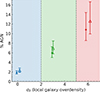 |
Fig. A.1. Variations in the AGN fraction (in %) with local overdensity (σδ) for all different types of AGN combined at 2 < z < 4 in an 80% stellar-mass (M* > 109.14 M⊙) complete in our redshift range (open triangle points). The stellar mass distribution of galaxies remains roughly the same across different environment bins. The median log M*/M⊙ values for the three environment bins (left to right in the figure) are: 9.60, 9.77, and 9.66, respectively. The circle points and σδ bins are same as in Figure 6. The figure shows a clear trend of increasing AGN fraction with increasing local overdensities of galaxies. |
Appendix B: Mass distribution of peaks and their structures
In Sect. 3.2, for probing the variation in AGN fraction with global environment, we used 5σδ peaks with total mass (M5σδ) of Mtot > 1012.8 M⊙. Our analysis (See Figure B.1 and Figure B.2) show that most of such systems have M5σδ > 1013 M⊙ and they are embedded within broader 2.5σδ envelopes with masses M2.5σδ > 1014 M⊙. Therefore this observations suggest that the such 5σδ samples generally represent the cores of protoclusters. In Figure B.1, we display the mass distribution of the 5σδ peaks alongside that of the corresponding 2.5σδ envelopes in which they reside. In Figure B.2, we plot the ratio of M2.5σδ to M5σδ as a function of M5σδ. In both figures, we divided the X-axis into bins of unit width. For each bin, we calculated the median y value, with error bars representing the Normalized Median Absolute Deviation (NMAD). The consistent behavior of this mass ratio across bins further supports our interpretation of the 5σδ cores being embedded within massive protocluster envelopes.
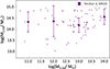 |
Fig. B.1. Distribution of the total mass of 5σδ peak and their corresponding 2.5σδ envelopes (cross points). The x-axis is divided into bins of unit width. For each bin, the median y-value is shown by filled purple circle. The error bars on these points correspond to the Normalized Median Absolute Deviation (NMAD) of the points in that bin. The plot shows that most of massive M5σδ > 12.8 reside in protoclusters with M2.5σδ > 1014 M⊙. |
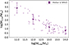 |
Fig. B.2. Distribution of the total mass of 5σδ peak and the ratio of mass of 5σδ to their corresponding 2.5σδ envelopes (cross points). We divided the X-axis into bins of unit width. For each bin, the median value of mass-ratio is shown by filled purple circle. The error bars correspond to the NMAD of the points in the given bin. The plot shows that most of massive M5σδ > 12.8 reside much in protoclusters that have mass almost an order of magnitude higher compared to the M5σδ peaks. |
All Figures
|
Fig. 1. Redshift distribution of all 901 AGNs in the Lyu et al. (2022) catalog (purple histogram). This large AGN dataset includes all nine categories of AGN defined in Lyu et al. (2022). Note: the categories are not mutually exclusive, i.e., a given AGN can satisfy the selection criteria for multiple categories of AGNs. The redshift values for these AGNs are sourced from the Lyu et al. (2022) catalog. We also overplotted the redshift distribution of 591 Lyu et al. (2022) AGNs that are matched with the C3VO (MUSYC) sources within a projected separation of 0.5 (orange histograms with purple lines). The redshift distribution peaks around z ∼ 0.75, and almost vanishes at z > 4. In this study, we restricted our analysis to the redshift range of 2.0 < z < 4.0 as shown by the gray shaded region between the two black dashed vertical lines. |
| In the text | |
|
Fig. 2. Distribution of the observed X-ray luminosity (Lxobs) vs. redshift (z) for all 658 sources in Lyu et al. (2022) with Lxobs > 0.0 (purple filled circles). Out of them, the 435 sources that are matched to the C3VO sources within a separation of 0.5″ are highlighted (purple filled circles with orange edge colors). The redshifts for the Lyu et al. (2022) sources are from their AGN catalog, which are sourced from the 3D-HST catalog. For this study, we only focused on redshift range of 2.0 < z < 4.0 as shown by the gray shaded region between the two black dashed vertical lines. |
| In the text | |
|
Fig. 3. Distribution of redshift vs. σδ (local galaxy overdensity) for 120 525 objects with 2.0 < zgal < 4.0 across the 100 Monte Carlo realizations. The number of objects is approximately 100 times higher than the true number of galaxies, averaging around 1205 objects per Monte Carlo iteration. The scatter points represent galaxies with their MC realization-specific local overdensity (σδ): coeval field (σδ < 2.0) (blue points), intermediate overdensities (2.0 < σδ < 5.0) (green points), and highly overdense peaks (σδ > 5.0) (red points). The histograms on top show the σδ distribution and the histograms on right show the redshift (zgal) for the three σδ bins: σδ < 2.0 (solid blue line), 2.0 < σδ < 5.0 (dashed green line), and σδ > 5.0 (dotted red line). The dashed gray lines show the division of the local overdensity in the three different bins used in our analyses. We also write the given names (gray text) of all five spectroscopically confirmed massive (Mtot ≥ 1014.8 M⊙) protostructures that are at z < 4 as presented in Shah et al. (2024) along with their redshift extent (horizontal dashed lines above and below the protostructure names). Furthermore, we also show the redshift of the most massive (Mtot = 1014.7 M⊙) protostructure in 2.0 < z < 4.0, which is located at z ∼ 2.45, and spread over 2.40 < z < 2.48. The broad horizontal stripe at z ∼ 3.05 consists of four protostructures, each less massive than those discussed in Shah et al. (2024). Likewise, the stripe at z ∼ 2.05 corresponds to a single protostructure with lower mass than the z ∼ 2.45 structure reported in this paper. Signs of these additional structures are visible in the figure above, but are not discussed in detail in Shah et al. (2024) or in the present paper due to their lower masses. |
| In the text | |
|
Fig. 4. Total mass distribution of massive (Mtot > 1012 M⊙) structures (contiguous envelope consisting of voxels with σδ > 2.5) in three different redshift bins: 2.0 < z < 2.5 (navy solid line), 2.5 < z < 3.0 (turquoise dashed line), and 3.0 < z < 4.0 (pink dotted line). |
| In the text | |
|
Fig. 5. 3D distribution of local overdensity in ECDFS, highlighting the most massive protostructure (Mtot = 1014.7 M⊙) at z ∼ 2.45, spread over 2.40 < z < 2.48. The protostructure encapsulates two massive (Mtot > 1013.25 M⊙) overdensity peaks (σδ > 5.0) shown as P1 and P2. |
| In the text | |
|
Fig. 6. Variations in the AGN fraction (in %) with local overdensity (σδ) for all different types of AGNs combined at 2 < z < 4. The σδ is divided into three different bins – (i) σδ < 2.0 (blue): coeval field, (ii) 2.0 < σδ < 5.0 (green): intermediate overdensity, (iii) σδ > 5 (red): highest overdensity peaks. The figure shows a clear trend of an increasing AGN fraction with the increasing local overdensities of galaxies. |
| In the text | |
|
Fig. 7. AGN fraction (in %) for the different types of AGN in different overdensity bins: coeval field (blue) intermediate overdensity (green), and highest overdensity peaks (red). Here, we only show the five categories (MIR-SED, MIR-color, X-ray-lum, X2R, and opt-sp) for which, on average, there are more than eight AGNs across all 100 MC iterations. Note: the categories are not mutually exclusive and an AGN may meet the criteria for more than one category. See Figure 11 in Lyu et al. (2022) for the overlap of sources in different AGN categories. The asymmetric 1σ errors on these AGN fractions are shown. For all categories, there is a clear trend of higher AGN fraction for galaxies in denser environments. |
| In the text | |
|
Fig. 8. Variations in the AGN fraction (in %) with local overdensity (σδ) for all different types of AGN combined at 2 < z < 4 in two different mass bins divided at M* = 1010.2 M⊙. The σδ bins are the same as in Figure 6. The diamond points correspond to galaxies with M* > 1010.2 M⊙ and star points correspond to galaxies with M* < 1010.2 M⊙. The figure shows a clear trend of an increasing AGN fraction with the increasing local overdensities of galaxies in both stellar mass bins. |
| In the text | |
|
Fig. 9. Variations in the AGN fraction (in %) with local overdensity for all different types of AGN combined in three different redshift bins of 2.0 < z < 2.5 (navy squares), 2.5 < z < 3.0 (cyan triangles), and 3.0 < z < 4.0 (pink pentagons). Almost all points show a higher AGN fraction in denser environments at all redshifts. |
| In the text | |
|
Fig. 10. AGN fraction (in %) as a function of global environment Rproj, norm = Rproj/Reff (red points), where Rproj is the projected distance of the galaxy from its nearest 5σδ peak and Reff is the effective radius of the corresponding 5σδ peak. The solid black line is the AGN fraction value for the corresponding coeval field, with its 1σ errors shown using dashed black lines. |
| In the text | |
|
Fig. A.1. Variations in the AGN fraction (in %) with local overdensity (σδ) for all different types of AGN combined at 2 < z < 4 in an 80% stellar-mass (M* > 109.14 M⊙) complete in our redshift range (open triangle points). The stellar mass distribution of galaxies remains roughly the same across different environment bins. The median log M*/M⊙ values for the three environment bins (left to right in the figure) are: 9.60, 9.77, and 9.66, respectively. The circle points and σδ bins are same as in Figure 6. The figure shows a clear trend of increasing AGN fraction with increasing local overdensities of galaxies. |
| In the text | |
|
Fig. B.1. Distribution of the total mass of 5σδ peak and their corresponding 2.5σδ envelopes (cross points). The x-axis is divided into bins of unit width. For each bin, the median y-value is shown by filled purple circle. The error bars on these points correspond to the Normalized Median Absolute Deviation (NMAD) of the points in that bin. The plot shows that most of massive M5σδ > 12.8 reside in protoclusters with M2.5σδ > 1014 M⊙. |
| In the text | |
|
Fig. B.2. Distribution of the total mass of 5σδ peak and the ratio of mass of 5σδ to their corresponding 2.5σδ envelopes (cross points). We divided the X-axis into bins of unit width. For each bin, the median value of mass-ratio is shown by filled purple circle. The error bars correspond to the NMAD of the points in the given bin. The plot shows that most of massive M5σδ > 12.8 reside much in protoclusters that have mass almost an order of magnitude higher compared to the M5σδ peaks. |
| In the text | |
Current usage metrics show cumulative count of Article Views (full-text article views including HTML views, PDF and ePub downloads, according to the available data) and Abstracts Views on Vision4Press platform.
Data correspond to usage on the plateform after 2015. The current usage metrics is available 48-96 hours after online publication and is updated daily on week days.
Initial download of the metrics may take a while.