| Issue |
A&A
Volume 704, December 2025
|
|
|---|---|---|
| Article Number | A188 | |
| Number of page(s) | 12 | |
| Section | Stellar structure and evolution | |
| DOI | https://doi.org/10.1051/0004-6361/202554393 | |
| Published online | 09 December 2025 | |
Ensemble seismic study of the properties of the core of red clump stars
1
Institut de Ciencies de l’Espai (ICE, CSIC), Carrer de Can Magrans S/N, 08193 Bellaterra, Spain
2
Institut d’Estudis Espacials de Catalunya (IEEC), Carrer Gran Capita 4, 08034 Barcelona, Spain
3
Heidelberger Institut für Theoretische Studien, Schloss-Wolfsbrunnenweg 35, 69118 Heidelberg, Germany
4
Department of Astronomy, Yale University, PO Box 208101, New Haven, CT 06520-8101, USA
5
Center for Astronomy (ZAH/LSW), Heidelberg University, Königstuhl 12, 69117 Heidelberg, Germany
★ Corresponding author: This email address is being protected from spambots. You need JavaScript enabled to view it.
Received:
6
March
2025
Accepted:
7
October
2025
Abstract
Context. Red clump (RC) stars still pose open questions regarding several physical processes, such as the mixing around the core or the nuclear reactions, which are ill-constrained by theory and experiments. The oscillations of RC stars, which are of a mixed gravito-acoustic nature, allow us to directly investigate the interior of these stars and thereby better understand their physics. In particular, the measurement of their period spacing is a good probe of the structure around the core.
Aims. We aim to explain the distribution of period spacings in RC stars observed by Kepler by testing different prescriptions of core-boundary mixing and the nuclear reaction rate.
Methods. Using the MESA stellar evolution code, we computed several grids of core-helium-burning tracks, with varying masses and metallicities. Each of these grids has been computed assuming a certain core boundary mixing scheme, or 12C(α, γ)16O reaction rate. We then sampled these grids, in a Monte-Carlo fashion, using observational spectroscopic metallicity and seismic mass priors, in order to retrieve a period spacing distribution, which we compared to the observations.
Results. We find that the best-fitting distribution is obtained when using a “maximal overshoot” core-boundary scheme, which has similar seismic properties as a model whose modes are trapped outside a semi-convective region, and which does not exhibit core-breathing pulses at the end of the core-helium-burning phase. If no mode trapping is assumed, then no core boundary mixing scheme is compatible with the observations. Moreover, we find that extending the core with overshoot worsens the fit. Additionally, reducing the 12C(α, γ)16O reaction rate (by around 15%) improves the fit to the observed distribution. Finally, we note that an overpopulation of early RC stars with period spacing values around 250 s is predicted by the models but not found in the observations.
Conclusions. Assuming a semi-convective region and mode trapping, along with a slightly lower than nominal 12C(α, γ)16O rate, allowed us to reproduce most of the features of the observed period spacing distribution, except for those of early RC stars.
Key words: asteroseismology / convection / nuclear reactions / nucleosynthesis / abundances / stars: evolution / stars: horizontal-branch / stars: interiors
© The Authors 2025
 Open Access article, published by EDP Sciences, under the terms of the Creative Commons Attribution License (https://creativecommons.org/licenses/by/4.0), which permits unrestricted use, distribution, and reproduction in any medium, provided the original work is properly cited.
This article is published in open access under the Subscribe to Open model. This email address is being protected from spambots. You need JavaScript enabled to view it. to support open access publication.
1. Introduction
The red clump (RC) is composed of low-mass (approximately less than 1.8 M⊙) stars that have gone through the helium flash and are currently in the core-helium-burning (CHeB) stage. An interesting aspect of these RC stars is that their luminosity and, more generally, the properties of their core depend little on the mass of the star or on pre-CHeB evolution. Therefore, they can be used as standard candles and/or tracers of the evolution of the composition of the Galaxy (see the review by Girardi 2016).
Yet, the structures of RC stars are not fully understood, due to the lack of theoretical prescriptions for several physical processes. In particular, the properties of core boundary mixing (CBM) are ill-defined by theory (Castellani et al. 1971a,b; Bressan et al. 1986). Furthermore, the determination of the nuclear reaction rate of the 12C(α, γ)16O reaction, despite having progressed significantly the last decades, is still subject to significant uncertainties (Kunz et al. 2002; deBoer et al. 2017; Shen et al. 2023).
Asteroseismology provides a way to put observational constraints on these physical processes. RC stars are solar-like oscillators, i.e., their modes are excited by the turbulent motion of fluid in the convective envelope. Moreover, their non-radial modes are mixed: they propagate as gravity waves in a region contained around the convective core and as pressure waves in the outer part of the star. Because of this, these modes are particularly sensitive to the properties of the region around the convective core. A key aspect of the mixed modes of evolved post-main sequence stars, such as RC stars, is that they closely follow an asymptotic relation (Shibahashi 1979). This has allowed us to define a period spacing, ΔΠ, that is a direct probe of the region around the convective core. Thanks to the data from the Kepler satellite (Borucki et al. 2010), the period spacing of thousands of RC stars has been measured (Mosser et al. 2012, 2014; Vrard et al. 2016), which opened a new window to the internal properties of these stars. Notably, Montalbán et al. (2013) showed that extending the convective core beyond the boundary defined by the Schwarzschild criterion is necessary to reproduce observations. The question of the nature of the CBM has been investigated by several works, with varying results: ad hoc “maximal” extension of the core (Constantino et al. 2015), as well as mild extension of the core with a radiative (Bossini et al. 2015) or adiabatic (Bossini et al. 2017) temperature stratification. Moreover, Noll et al. (2024) (N24 hereafter) find that a straightforward core extension, such as overshooting or penetrative convection, could not explain the seismic observations. This result, which differs from that of Bossini et al. (2015, 2017), is due to the fact that N24 used a different algorithm to determine the convective boundaries. Specifically, they used the convective premixing scheme, which ensures convective neutrality at the boundaries, following the recommendations of Gabriel et al. (2014). Furthermore, similarly to Constantino et al. (2015, 2017), N24 evoked the possibility that the observed modes could be trapped outside the CBM region, which would impact the observed period spacing. Additionally, these authors show that the rate of the 12C(α, γ)16O reaction, when increased, lengthens the duration of the CHeB phase such that the maximum value of period spacing reached by the models increases. All of these investigations show the strong potential of asteroseismology, and in particular the study of period spacing, to better understand the physics of RC stars.
For this work, we performed an ensemble study of the period spacings of a sample of RC stars observed by Kepler. To do so, we simulated the observed distribution of period spacings, taking into account the variations of metallicity and mass within the sample and using different prescriptions of the physics of the models. The aim is to test the validity of these prescriptions, by comparing the distribution of the models’ period spacings with the observed one. In Sect. 2, we introduce the method as well as the properties of the models used in this work. We then show in Sect. 3 how the distributions that we obtained assuming different physics compare with the observed one. Next, in Sect. 4, we discuss the so-called 250 s peak, which is the largest difference between the modeled distribution and the observations. Finally, we conclude in Sect. 5.
2. Method
For this work, we performed Monte-Carlo simulations of the period spacing distribution observed by the Kepler satellite, and whose properties are described in Section 2.1. To do so, for each physical assumption (on core boundary mixing or nuclear reaction rates), we computed a grid of models with varying masses and metallicities. The properties of these grids are presented in Sect. 2.2.1. We then randomly sampled these grids of tracks using age, mass, and metallicity priors that are similar to those of the Kepler sample, as detailed in Sect. 2.3. The resulting period spacing distribution was finally compared to the observations.
2.1. Properties of the observed sample
The observational sample that we used for this work was taken from the crossmatch of the data from the APOKASC-3 catalog (Pinsonneault et al. 2025) and Vrard et al. (2016). The period spacing values were taken from Vrard et al. (2016), the masses from the seismic values of Pinsonneault et al. (2025), and the metallicities and alpha-enrichment values from the spectroscopic data of the same work, which were taken from APOGEE DR16 and DR17 (Ahumada et al. 2020; Abdurro’uf et al. 2022). The metallicity values have been altered to take the effect of α enrichment into account, following the prescription from Salaris et al. (1993), with coefficients having been recomputed in order to match the Grevesse & Sauval (1998) mixture used in the models [Fe/H]mod = [Fe/H]obs + log(0.683×10[α/Fe]+0.320).
From this sample, we only considered stars whose values of mass and metallicity are covered by our grids of models (see Sect. 2.2.1): masses between 0.8 and 1.8 M⊙, and metallicities between −0.8 dex and 0.4 dex. Furthermore, we applied an uncertainty cut and only included stars for which the quoted uncertainty on the period spacing is less than 6 s. The final sample consists of 2110 stars.
Figure 1 shows the observed period spacing distribution. The uncertainties of the bin counts were computed taking the observational uncertainties into account, following the approach explained in Appendix A.
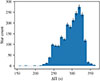 |
Fig. 1. Period spacing distribution of the observed sample (data from Vrard et al. 2016). The uncertainties were computed following the procedure described in Appendix A. |
2.2. Properties of the models
2.2.1. Microphysics
The models used for this work were computed with the MESA stellar evolution code, revision 22–11.1 (Paxton et al. 2011, 2013, 2015, 2018, 2019; Jermyn et al. 2023), with physics similar to N24. The opacities were computed using the OPAL code (Iglesias & Rogers 1996). The equation of state is a mixture of FreeEOS (Irwin 2012) and Skye (Jermyn et al. 2021). The convection model comes from Kuhfuss (1986). The mixing-length parameter has been fixed to 1.8, and it was not varied as it does not impact the properties of the core and therefore the period spacing. The nuclear reaction rates are from the REACLIB database (Cyburt et al. 2010), and in particular from Xu et al. (2013) for the 12C(α, γ)16O reaction. We took all of the reactions of the pp chain into account, as recommended by Noll & Deheuvels (2023). Finally, we used the solar mixture from Grevesse & Sauval (1998).
2.2.2. Core boundary mixing
In this section, we briefly describe the four core boundary mixing assumptions that we tested for this work. For more details, we refer the reader to N24.
2.2.2.1. Semi-convection:
The region outside the fully mixed part of the core is semi-convective, i.e., the composition is such that ∇rad = ∇ad, with ∇rad and ∇ad being the radiative and adiabatic gradients, respectively. The presence of such a region in CHeB stars was first predicted by Schwarzschild & Härm (1969) and studied more thoroughly in Castellani et al. (1971a,b). As its definition differs from a parametrized semi-convection model, similar to the one of Langer et al. (1983), it is often referred to as induced semi-convection. For this work, we obtained such semi-convective regions using the convective premixing scheme (Paxton et al. 2019). We note that for many tracks with semi-convection included, we found core-breathing pulses (CBPs) at the end of the CHeB phase. More details on this process are given in Sect. 2.2.3.
2.2.2.2. Overmixing:
The convective core is extended over a distance dov = αovHp, with αov being a free parameter and Hp the pressure scale height. The temperature gradient is considered to be ∇ = ∇rad in the overshoot region, with ∇ being the temperature gradient. Since we used the convective premixing scheme to determine the convective boundaries, a semi-convective region occured around the overshoot region for the more evolved models, as described in N24. We note that, in order to ensure that ∇rad = ∇ad in the semi-convective region beyond the overshoot region, we added a supplementary call to the convective premixing routine in MESA, which was done after the burning1. Overmixing models exhibit CBPs at the end of the CHeB phase. To suppress these, we neglected the gravitational energy term in the energy equation, following the recommendations of Dorman & Rood (1993) (see Sect. 2.2.3).
2.2.2.3. Penetrative convection:
This scheme is similar to the overmixing scheme, but the temperature gradient was set to ∇ = ∇ad in the overshooting region. For penetrative convection models as well, we neglected the gravitational energy term in the energy equation.
2.2.2.4. Maximal overshoot (MO):
Once a local minimum appeared in the radiative gradient profile, we defined the core size such that this local minimum was equal to the adiabatic gradient. This scheme, which was introduced in Constantino et al. (2015), is by definition nonphysical: the value of the radiative gradient at the outer boundary of the mixed region is significantly larger than the adiabatic gradient. However, as shown in Appendix B, it gives a similar period spacing as a model with an induced semi-convective region and observed modes that are trapped outside of the semi-convective region. Yet, contrary to the semi-convective models, models computed with maximal overshoot do not show CBPs.
2.2.3. Handling the CBPs
Core-breathing pulses are sudden increases of the convective core size that occur at the end of the CHeB phase. They are caused by the fact that, when the central helium abundance Yc is low, a small intake of helium results in a large relative variation in the helium abundance in the core. This leads to a significant increase in the energy production and hence of the core size (Sweigart & Demarque 1972). CBPs seem to be a numerical artifact rather than an actual instability happening inside stars. Their occurrence does indeed depend on the precision of the grid or timestep (Dorman & Rood 1993), and they are suppressed when using a nonlocal implementation of the mixing (Bressan et al. 1986) or when taking a maximum helium ingestion rate into account (Spruit 2015; Constantino et al. 2017). Moreover, observations of the ratio between asymptotic giant branch and horizontal branch stars in clusters (Caputo et al. 1989; Constantino et al. 2016) and of the period spacing in asteroseismology (Constantino et al. 2015; Noll et al. 2024) are not aligned with predictions coming from models that include CBPs.
Therefore, we decided to suppress CBPs in models that include overshoot. To do so, we followed the approach of Dorman & Rood (1993), in which the authors forced the models to be at thermal equilibrium by neglecting ϵg ≡ −Tds/dt, with T being the temperature, s the specific entropy, and t the time. The reason for that is that the extension of the core, caused by the increase in the energy production, leads to a negative ϵg at the core boundary, which in turn extends the core even more, causing a runaway extension. By neglecting this term, the CBPs are rapidly damped.
To investigate how neglecting ϵg affects the evolution of period spacings, we computed the evolution of ΔΠ for different CBM, with and without neglecting ϵg. The evolution of the period spacing for these models is shown in Fig. 3. One can see that models computed without taking ϵg into account do not exhibit CBPs at the end of the CHeB phase, while the effect on the rest of the CHeB phase is negligible. Moreover, we added the evolution of ΔΠ for a maximal overshoot model. Even though we consistently included ϵg in the computation of these models appearing in the rest of the work, it serves here as a reference case to investigate the effect of neglecting ϵg. Thus, we find that it has little impact during most of the CHeB phase except for the very end, during the core contraction. These differences occur during a small fraction of the CHeB phase, such that the final effect on the simulated ΔΠ distributions is small. Finally, we got rid of the residual CBPs if they happened at the very end of the helium-burning phase (Yc < 0.015).
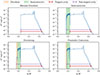 |
Fig. 2. Brunt-Väisälä profiles of four models with different CBM schemes, which were all stopped at Yc = 0.3. We indicate the overshoot region in orange, which is fully chemically mixed with the convective core. The region in green indicates the semi-convective region, where ∇rad = ∇ad. Finally, we indicate the region over which N/r was integrated in the trapped mode scenario (red) and in the non-trapped mode scenario (purple). |
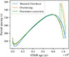 |
Fig. 3. Evolution of the period spacing during the CHeB phase for models computed with (dashed line) and without taking ϵg into account in the energy equation (full line). |
2.3. Properties of the grids and sampling priors
The models in each of the grids have been computed to have masses between 0.8 and 1.8 M⊙, in steps of 0.2 M⊙, and with metallicities [Z/X]0 between −0.8 and 0.4 dex, in steps of 0.2 dex. The initial helium abundance Y0 was computed using a commonly used enrichment law Y0 = 0.24 + 2 Z0.
We sample the period spacings of these tracks in a Monte-Carlo fashion, with mass, metallicity, and age priors being as close as possible to the ones of the observed sample. Regarding age, we define τ a “normalized” CHeB age, that is to say, an affine transformation of the age of the star such that τ = 0 at the start of the CHeB phase and τ = 1 at the end. Our prior in τ is then uniform between 0.01 and 0.99. For the mass and the metallicities, we used the seismic and spectroscopic observation distributions from Pinsonneault et al. (2025), respectively. The metallicity values have been altered to take the α enrichment into account, as explained in Sect. 2.1. We then performed an inverse transform sampling to obtain a set of masses and metallicity values that have the same distribution as the observational priors.
To obtain the period spacings corresponding to the values of τ, masses, and metallicities randomly drawn as described above, we performed 3D linear interpolations of the period spacing within the grid. To simulate the observational period spacing uncertainties, we perturbed the values obtained through the interpolation by adding a realization of 𝒩[0,σ2(ΔΠ)], with 𝒩 being the normal distribution. We modeled the uncertainty σ(ΔΠ) as a linear function of ΔΠ, fitted to the actual observational uncertainties, as shown in Fig. 4. This allowed us to take the correlation between the uncertainties and the period spacing into account. Moreover, in the case of the models computed in the “non-trapped” scenario (see Sect. 2.5), the evolution of the period spacing is slightly noisy (see, e.g., Fig. 4 of Noll et al. 2024). Thus, for these models, we added in quadrature a numerical noise of 1 s. For each test presented in Sect. 3, we performed 100 000 realizations.
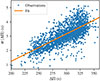 |
Fig. 4. Period spacing uncertainties of the sample of Vrard et al. (2016), plotted against the period spacing values of the same work. The orange line shows the linear fit that we used to simulate the uncertainties in our simulations. |
To quantify the uncertainties of the histograms of the synthetic sample, we performed a Monte-Carlo approach. Thus, we repeated the sampling procedure described above 700 times, and considered, for each bin, the standard deviation of the resulting values as the uncertainty.
2.4. Comparing the surface properties of the observed data and the simulated sample
To verify that our sampling is compatible with the observed sample, we performed a simulation of the Hertzsprung-Russell diagram of our sample. To do so, we followed a similar methodology as the one described in Sect. 2.3, and perturbed the obtained values of effective temperatures and luminosities by adding a Gaussian uncertainty of 50 K and 5 L⊙, respectively. Observational values of effective temperatures were taken from the APOGEE DR17 sample, and the luminosities from Berger et al. (2018). The latter encompasses 2063 stars out of the 2110 stars of the observational sample used elsewhere in this work.
In Fig. 5, we present the kernel density estimation (KDE) of the effective temperature and luminosities of the synthetic and observational samples. In order to correct for the systematic shift between the two, we subtracted the median of each sample. The differences between the median value of the synthetic and observed samples are −164 K for the effective temperature and −2.23 L⊙ for the luminosity. The first may be attributed to the fact that we computed models with a fixed value for the mixing-length parameter, while the second is smaller than the typical observational uncertainties.
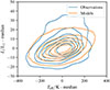 |
Fig. 5. Kernel density estimations of the distributions of luminosities and effective temperature of the observed (blue) and synthetic (orange) samples, substracted by the median value of the sample. |
We find that the range of effective temperature and luminosities covered by our simulations is compatible with the one of the observations, hence showing the consistency between the synthetic and observed samples. We also find that the observed sample has a higher number of stars with high luminosities, but we note that most of these stars have a large (> 10 L⊙) luminosity uncertainty.
2.5. Computing period spacings
The period spacings ΔΠ of dipole modes were computed for this work using the asymptotic formulation of Shibahashi (1979), namely:
 (1)
(1)
with r0, 1 being the boundaries of the g-mode resonating cavity, N the Brunt-Väisälä frequency, and r the radial coordinate.
The boundaries of the g-mode cavity are determined differently depending on whether mode trapping is taken into account or not. In the first case, r0 was taken at the outermost radius of the maximal overshoot, overmixing, or semi-convective region, depending on the CBM scheme. At this position, there is indeed a steep helium discontinuity, which can reflect waves such that most of the oscillating energy of the observed modes is situated beyond r0. Using such a lower boundary allowed us to compute a period spacing that is consistent with the frequencies computed using a stellar oscillation code (see Appendix D). Moreover, such an approach is similar to the one used in Constantino et al. (2017). We note that, in this “mode-trapping” scenario, the value of the period spacing is independent of the chemical and thermal stratification within the CBM region, but it is still sensitive to the radial extent of the CBM region.
In the second scenario, we did not take mode trapping into account. Therefore, we define r0 as the inner boundary of the G-mode cavity, i.e., where, formally, N2 > ωn, l, with ωn, l being the angular frequency of the mode (Shibahashi 1979). In our case, as the angular frequencies of the observed modes are situated around the angular frequency of maximum oscillation power ωmax, we define r0 as the radius where N2 > ωmax. We computed ωmax using the scaling relation ωmax = ωmax, ⊙(M/M⊙)(R/R⊙)−2(Teff/Teff, ⊙)−0.5 (Kjeldsen & Bedding 1995). In that case, contrary to the mode-trapping case, it is directly sensitive to the stratification in temperature and composition inside the CBM region. Finally, in both cases, r1 is defined as the outermost radius where N2 > ωmax2.
Typical Brunt-Väisälä profiles for the four different CBM scenarios are presented in Fig. 2. We indicate the region over which N/r was integrated in the trapped scenario in red and in the non-trapped scenario in purple.
3. Results
In this section, we first present the period spacing distributions that we obtained for different core boundary mixing scenarios, assuming either the presence or the absence of mode trapping (in Sect. 3.1 and 3.2, respectively). Then, in Sect. 3.3, we investigate the effect of varying the rate of the 12C(α, γ)16O reaction on the distributions.
3.1. In the presence of mode trapping
In this section, we explain how we computed the period spacing in the mode-trapping scenario, as described in Section 2.5. Figure 6 shows the distributions of period spacing computed with four different CBM schemes. The best-fit models are the ones constructed by using the maximal overshoot scheme, which is able to reproduce the main properties of the observed period spacing distributions. Yet, we can note that there is an overestimation of models with high values of period spacing (> 325 s), which can be resolved by decreasing the rate of the 12C(α, γ)16O reaction (see Sect. 8). Also, we observed two other features that are not reproduced by the models: a significant peak is present in the models around 250 s but not in the observations. The origin of this peak is discussed in Sect. 4. Also, around 290 s, an observational bin has a value significantly higher than the one predicted from the models. These two features are the main differences between the models and the observations.
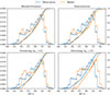 |
Fig. 6. Distributions of the computed values of period spacing (orange) and of the observed values of period spacing (blue), for models that assume mode trapping. The lines represent the corresponding cumulative distributions. The simulated distributions were computed using a maximal overshoot scheme (upper left), a semi-convection scheme (upper right), and an overmixing scheme with αov = 0.2 (lower left) and αov = 0.5 (lower right). The represented bin uncertainties for the observations were computed following the procedure explained in Appendix A. Each bin value and associated uncertainties were normalized, i.e., divided by the total count and the bin width. |
The semi-convection scheme yields a poorer fit because of the CBPs that occur in these models. CBPs do indeed lead to a significant number of realizations with very high values of period spacing (400 s, not visible in this plot) as well as a lower number of realizations around 300 s, compared to the distribution resulting from maximal overshoot. Both of these features are not in line with the observed distributions.
Regarding the core extent, only period spacings computed using an overmixing scheme for the two values of 0.2 and 0.5 for αov are represented in Fig. 6. We can see that adding overshoot yields a poorer fit to the observations compared to maximal overshoot. Notably, due to the extension of the core, the predicted number of models with low values of period spacing (from 225 to 250 s) is significantly lower than the one observed in the Kepler data. Also, for models computed with a large value for αov, there is a strong overestimation of the number of stars with higher values for period spacing. This is not the case for αov = 0.2, where the predicted number of stars at high values for period spacing is similar to the maximal overshoot case. This is due to the fact that during the late CHeB phase, the extent of the CBM region (i.e., overshoot and semi-convection) of models with αov = 0.2 is similar to the extent of the fully mixed region of maximal overshoot models.
3.2. In the absence of mode trapping
In this section, we explain how we computed the period spacing as in the “non-trapped” case, i.e., integrating over the full g-mode cavity region. The results of our computations are shown in Fig. 7. We focus on the cases of overmixing and penetrative convection, as the results are similar for maximal overshoot models and they significantly deviate from the observations for semi-convective models (see Fig. 9 of N24). A striking result is that regardless the value for αov or the kind of temperature stratification in the overshoot region, none of these schemes can reproduce the observations if no mode trapping is assumed. In the case of overmixing, even with a high value for αov, the simulated distributions underestimate the number of high period spacing models. Regarding penetrative convection, the distributions computed with a low or high value for αov are both incompatible with the highest and lowest values for observed period spacings. No “sweet-spot” value for αov allowed us to produce a distribution that is compatible with the observations.
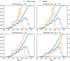 |
Fig. 7. Same as in Fig. 6, but without considering mode trapping, i.e., with period spacings being computed in the full g-mode cavity. |
A potential way to solve this discrepancy would be a temperature stratification that evolves during the CHeB phase, such that it is radiative at first and then adiabatic. Also, an evolving value for αov could improve the fit, if using penetrative convection. However, the study of such parametrization, which would lead to a very extended parameter space, is beyond the scope of this paper.
3.3. 12C(α, γ)16O nuclear reaction rates
To test nuclear reaction rates, we computed all our models using the maximal overshoot scheme as it is the one that is the most compatible with the observations. The rates were varied by multiplying the nominal value from Xu et al. (2013) by a given value. A comparison between the values of the different nuclear rates computed in this work and the recommendations from deBoer et al. (2017) are shown in Fig. C.1.
Fig. 8 shows the computed distributions for different rates of the 12C(α, γ)16O reaction. The effect is, as expected from N24, lower than the one resulting from varying the CBM prescription. We find that a higher rate leads to a larger number of predicted models with high values for period spacing. This is a consequence of the increased maximum value of period spacing reached by models with a rate for 12C(α, γ)16O, as it lengthens the duration of the CHeB phase (N24). Decreasing the rate has the opposite effect. We observed that it improves the quality of fit, especially for the higher values for period spacing. In particular, multiplying the rate of 12C(α, γ)16O by 0.85 seems to yield the closest distribution. As one can see in Fig. C.1, this is approximately equivalent to the lower recommended rate of deBoer et al. (2017).
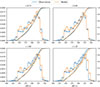 |
Fig. 8. Same as in Fig. 6, but for maximal overshoot and with varying 12C(α, γ)16O nuclear reaction rates. |
4. The peak at 250 s
In the best-fit case, the feature that dominates the differences between modeled and observed distributions is a peak around 250 s, which is visible, for instance, in the upper right panel of Fig. 8. As mentioned in Bossini et al. (2015)2, this peak is due to the behavior of the period spacing at the very start of the CHeB phase. At the very beginning of the CHeB phase, ΔΠ first decreases before continuously increasing until the final shrinking of the convective core, as illustrated in Fig. 9. Because of that initial decrease followed by an increase, the model spends more time with a period spacing around 250 s, and hence the overpopulation of models with such values for period spacing in the final simulated observations.
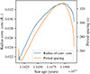 |
Fig. 9. Evolution of the radius of the convective core (blue) and of the period spacing (orange) for a 1 M⊙, maximal-overshoot model with solar metallicity, during the CHeB phase. |
We subsequently tried to understand the reason for such a decrease at the start of the CHeB phase. It is not due to a variation in the mass of the core: as shown in Fig. 9, the decrease in the mass of the core at the beginning of the CHeB phase happens too quickly to be compatible with the period spacing variation. Rather, as mentioned in Constantino et al. (2015), the decrease in period spacing is caused by the properties of the hydrogen-burning shell. To explore this, we show in Fig. 10 the evolution of the profile of the Brunt-Väisälä frequency at the location of the H-burning shell, at the very beginning of the CHeB phase. The bump, situated from 4.5 × 109 cm outward, is caused by the chemical gradient between the inner helium-rich region and the outer hydrogen-rich region. That bump is initially very narrow: this is a residual from the structure of the red giant branch, where the internal temperatures are high, and thus the energy production is particularly localized. This leads to a narrow transition between the helium-rich and hydrogen-rich regions, and thus a strong chemical gradient. However, during the CHeB phase, the temperatures are lower and therefore the H burning occurs in a larger region. This leads to a widening and flattening of the chemical composition gradient and thus the Brunt-Väisälä frequency, at the start of the CHeB phase when the structure of the star adapts to the new burning phase. Consequently, the value of the integral in Eq. (1) increases, leading to a decrease in period spacing. Once the chemical gradient of the H-burning shell reaches its final shape, the variations of the period spacing are dominated by the evolution of the convective core: ΔΠ increases.
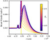 |
Fig. 10. Evolution of the Brunt-Väisälä frequency profile at the location of the H-burning shell, at the very start of the CHeB phase. The lines are colored following the central helium composition: evolution goes from yellow to purple. |
It is unclear why the 250 s peak does not appear in the observations. A selection effect due to peculiar global observables (such as luminosity, temperature, or large separation) is unlikely, as the early RC stars do not have distinct values for these compared to more evolved RC stars. However, as mentioned in Sect. 3.3 of Constantino et al. (2015), a potential bias could exist if the oscillation spectrum of these stars is messier than that of the other CHeB stars: it would be more difficult to measure the period spacing of a star with a messy power spectrum, which would automatically reduce their numbers in the sample of Vrard et al. (2016). Also, one can note the work of Singh et al. (2021), in which they measured the period spacing for super lithium-rich CHeB stars. They found several stars that are not part of the Vrard et al. (2016) sample and have a period spacing around 250 s.
Form a different perspective, the features of this peak can be influenced by the distribution in the initial helium abundance, Y0, of the sample. As can indeed be seen in Fig. 8 of N24, modifying Y0 has an impact on the value for the period spacing at the start of the CHeB phase, where the value for the period spacing is typically around 250 s. For this work, we assumed a fixed enrichment law, with a slope of 2. A larger variety in the initial helium abundance may somewhat smooth out the 250 s peak. We propose exploring this question in a future work.
Finally, as the 250 s peak is caused by the sharp Brunt-Väisälä profile at the beginning of the CHeB phase, we checked if microscopic diffusion may help smooth it. However, we found that the effect is negligible and it does not significantly impact the computed distributions.
5. Conclusions
For this work, we simulated the distribution of the period spacings of the RC stars of the Kepler sample, in order to test the validity of the core boundary mixing and 12C(α, γ)16O rates. To do so, for each core boundary mixing scheme or 12C(α, γ)16O reaction rate, we computed a grid of CHeB tracks using the MESA stellar evolution code, with varying values for metallicities and masses. We then drew samples from these grids with priors that are as close as possible to the observed sample: for the metallicity and the masses, we used the spectroscopic and seismic values, respectively, from Pinsonneault et al. (2025). For the age, we assumed that the stars are uniformly distributed along the CHeB phase. Finally, we perturbed the sampled period spacing values with uncertainties that are similar to the observational ones. This process allowed us to retrieve a period spacing distribution, which we compared to the observational one.
We found that we obtain the best fits when assuming a maximal overshoot mixing scheme. This scheme is, by definition, nonphysical, yet, it gives period spacing values that are equal to the ones of a model with an induced semi-convective region that does not exhibit any CBP and in which the observed modes are trapped outside the semi-convective region. The latter scenario, which is more physically justified, is our preferred interpretation of our results. We also found that adding overmixing, or penetrative convection, worsens the fit. Finally, we found that we cannot reproduce the observations if we compute the period spacings without taking the mode trapping into account, regardless of the mixing scheme used.
Regarding the rate of the 12C(α, γ)16O reaction, decreasing the nominal from Xu et al. (2013) by 15% slightly improves the fit to the observed distribution, by decreasing the number of stars with high values for period spacing. Such a decreased rate approximately corresponds to the lower recommended rate from deBoer et al. (2017).
Finally, we stress that the model distributions cannot reproduce all the features for the observations. The main difference is the so-called 250 s peak, which is an overpopulation of models with a period spacing around 250 s that is not found in the observations. This overpopulation is the result of the decrease in the period spacing at the very start of the CHeB phase, due to the adaptation of the structure of the H-burning shell to the CHeB phase: thus, its presence is well understood and not due to numerical artifacts. It is therefore unclear why such an overpopulation cannot be found in the observed sample: a possible explanation could be that the oscillation spectrum of the young RC stars that populate this 250 s population, which just passed through the helium flash, is too messy to allow any clear measurement of the period spacing. Also, a very wide variety in initial helium abundance within the Kepler sample could help “smoothen” the peak. Additional data from the PLATO mission (Rauer et al. 2014) could shed new light on this issue.
We noted that this supplementary call could lead to additional CBPs at the very end of the CHeB phase. Thus, we deactivated it in these cases.
Interestingly enough, the data distributions shown in Fig. 9 of Bossini et al. (2015), which were taken from Mosser et al. (2014), present a peak around 250 s. This peak is coincidental and caused by the smaller sample from Mosser et al. (2014). We did indeed find this peak back again when plotting the period spacing of the Mosser et al. (2014) subsample using the results from Vrard et al. (2016).
An equivalent plot can be found in Paxton et al. (2019), Fig. 44.
Acknowledgments
The authors thank the anonymous referee for their valuable comments, which helped improve the discussion and the overall clarity of the paper. AN thanks Simon Campbell for interesting discussions about the 250 s peak. AN and SH acknowledge funding from the ERC Consolidator Grant DipolarSound (grant agreement #10s1000296). SB acknowledges NSF grant AST-2205026. AN also acknowledges funding from the program Unidad de Excelencia Maria de Maeztu (CEX2020-001058-M), the Generalitat de Catalunya (2021-SGR-1526) and the Tecnologías avanzadas para la exploración del universo project, within the framework of NextGenerationEU PRTR.
References
- Abdurro’uf, Accetta, K., Aerts, C., et al. 2022, ApJS, 259, 35 [NASA ADS] [CrossRef] [Google Scholar]
- Ahumada, R., Allende Prieto, C., Almeida, A., et al. 2020, ApJS, 249, 3 [NASA ADS] [CrossRef] [Google Scholar]
- Berger, T. A., Huber, D., Gaidos, E., & van Saders, J. L. 2018, ApJ, 866, 99 [NASA ADS] [CrossRef] [Google Scholar]
- Borucki, W. J., Koch, D., Basri, G., et al. 2010, Science, 327, 977 [Google Scholar]
- Bossini, D., Miglio, A., Salaris, M., et al. 2015, MNRAS, 453, 2290 [Google Scholar]
- Bossini, D., Miglio, A., Salaris, M., et al. 2017, MNRAS, 469, 4718 [Google Scholar]
- Bressan, A., Bertelli, G., & Chiosi, C. 1986, Mem. Soc. Astron. It., 57, 411 [NASA ADS] [Google Scholar]
- Caputo, F., Castellani, V., Chieffi, A., Pulone, L., & Tornambe, A. J. 1989, ApJ, 340, 241 [NASA ADS] [CrossRef] [Google Scholar]
- Castellani, V., Giannone, P., & Renzini, A. 1971a, Ap&SS, 10, 355 [NASA ADS] [CrossRef] [Google Scholar]
- Castellani, V., Giannone, P., & Renzini, A. 1971b, Ap&SS, 10, 340 [NASA ADS] [CrossRef] [Google Scholar]
- Chidester, M. T., Farag, E., & Timmes, F. X. 2022, ApJ, 935, 21 [NASA ADS] [CrossRef] [Google Scholar]
- Constantino, T., Campbell, S. W., Christensen-Dalsgaard, J., Lattanzio, J. C., & Stello, D. 2015, MNRAS, 452, 123 [Google Scholar]
- Constantino, T., Campbell, S. W., Lattanzio, J. C., & van Duijneveldt, A. 2016, MNRAS, 456, 3866 [Google Scholar]
- Constantino, T., Campbell, S. W., & Lattanzio, J. C. 2017, MNRAS, 472, 4900 [NASA ADS] [CrossRef] [Google Scholar]
- Cyburt, R. H., Amthor, A. M., Ferguson, R., et al. 2010, ApJS, 189, 240 [NASA ADS] [CrossRef] [Google Scholar]
- deBoer, R. J., Görres, J., Wiescher, M., et al. 2017, Rev. Mod. Phys., 89, 035007 [NASA ADS] [CrossRef] [Google Scholar]
- Dorman, B., & Rood, R. T. 1993, ApJ, 409, 387 [NASA ADS] [CrossRef] [Google Scholar]
- Gabriel, M., Noels, A., Montalbán, J., & Miglio, A. 2014, A&A, 569, A63 [NASA ADS] [CrossRef] [EDP Sciences] [Google Scholar]
- Girardi, L. 2016, ARA&A, 54, 95 [Google Scholar]
- Grevesse, N., & Sauval, A. J. 1998, Space Sci. Rev., 85, 161 [Google Scholar]
- Iglesias, C. A., & Rogers, F. J. 1996, ApJ, 464, 943 [NASA ADS] [CrossRef] [Google Scholar]
- Irwin, A. W. 2012, FreeEOS: Equation of State for stellar interiors calculations, Astrophysics Source Code Library [record ascl:1211.002] [Google Scholar]
- Jermyn, A. S., Schwab, J., Bauer, E., Timmes, F. X., & Potekhin, A. Y. 2021, ApJ, 913, 72 [NASA ADS] [CrossRef] [Google Scholar]
- Jermyn, A. S., Bauer, E. B., Schwab, J., et al. 2023, ApJS, 265, 15 [NASA ADS] [CrossRef] [Google Scholar]
- Kjeldsen, H., & Bedding, T. R. 1995, A&A, 293, 87 [NASA ADS] [Google Scholar]
- Kuhfuss, R. 1986, A&A, 160, 116 [NASA ADS] [Google Scholar]
- Kunz, R., Fey, M., Jaeger, M., et al. 2002, ApJ, 567, 643 [CrossRef] [Google Scholar]
- Langer, N., Fricke, K. J., & Sugimoto, D. 1983, A&A, 126, 207 [NASA ADS] [Google Scholar]
- Mehta, A. K., Buonanno, A., Gair, J., et al. 2022, ApJ, 924, 39 [CrossRef] [Google Scholar]
- Montalbán, J., Miglio, A., Noels, A., et al. 2013, ApJ, 766, 118 [Google Scholar]
- Mosser, B., Goupil, M. J., Belkacem, K., et al. 2012, A&A, 540, A143 [NASA ADS] [CrossRef] [EDP Sciences] [Google Scholar]
- Mosser, B., Benomar, O., Belkacem, K., et al. 2014, A&A, 572, L5 [NASA ADS] [CrossRef] [EDP Sciences] [Google Scholar]
- Noll, A., & Deheuvels, S. 2023, A&A, 676, A70 [NASA ADS] [CrossRef] [EDP Sciences] [Google Scholar]
- Noll, A., Basu, S., & Hekker, S. 2024, A&A, 683, A189 [NASA ADS] [CrossRef] [EDP Sciences] [Google Scholar]
- Paxton, B., Bildsten, L., Dotter, A., et al. 2011, ApJS, 192, 3 [Google Scholar]
- Paxton, B., Cantiello, M., Arras, P., et al. 2013, ApJS, 208, 4 [Google Scholar]
- Paxton, B., Marchant, P., Schwab, J., et al. 2015, ApJS, 220, 15 [Google Scholar]
- Paxton, B., Schwab, J., Bauer, E. B., et al. 2018, ApJS, 234, 34 [NASA ADS] [CrossRef] [Google Scholar]
- Paxton, B., Smolec, R., Schwab, J., et al. 2019, ApJS, 243, 10 [Google Scholar]
- Pinsonneault, M. H., Zinn, J. C., Tayar, J., et al. 2025, ApJS, 276, 69 [NASA ADS] [CrossRef] [Google Scholar]
- Rauer, H., Catala, C., Aerts, C., et al. 2014, Exp. Astron., 38, 249 [Google Scholar]
- Salaris, M., Chieffi, A., & Straniero, O. 1993, ApJ, 414, 580 [NASA ADS] [CrossRef] [Google Scholar]
- Schwarzschild, M., & Härm, R. 1969, BAAS, 1, 99 [Google Scholar]
- Shen, Y., Guo, B., deBoer, R. J., et al. 2023, ApJ, 945, 41 [NASA ADS] [CrossRef] [Google Scholar]
- Shibahashi, H. 1979, PASJ, 31, 87 [NASA ADS] [Google Scholar]
- Singh, R., Reddy, B. E., Campbell, S. W., Kumar, Y. B., & Vrard, M. 2021, ApJ, 913, L4 [NASA ADS] [CrossRef] [Google Scholar]
- Spruit, H. C. 2015, A&A, 582, L2 [NASA ADS] [CrossRef] [EDP Sciences] [Google Scholar]
- Sweigart, A. V., & Demarque, P. 1972, A&A, 20, 445 [Google Scholar]
- Townsend, R. H. D., & Teitler, S. A. 2013, MNRAS, 435, 3406 [Google Scholar]
- Vrard, M., Mosser, B., & Samadi, R. 2016, A&A, 588, A87 [CrossRef] [EDP Sciences] [Google Scholar]
- Xu, Y., Takahashi, K., Goriely, S., et al. 2013, Nucl. Phys., 918, 61 [CrossRef] [Google Scholar]
Appendix A: Computation of the uncertainties of bins for observational data
In the histograms representing observational data, we took into account the observational uncertainties for the computation of the bin uncertainties, by computing them as follows.
For each bin j, each observation i can be considered as an independant Bernouilli trial, as the observation can be inside (“success”) or outside (“failure”) the bin bounds. We model the observed uncertainties as a normal distribution, 𝒩(xi, σi) with xi the observed value and σi the associated uncertainty. Then, the probability that the observation i is inside the bin j is:
![Mathematical equation: $$ \begin{aligned} p_i(j) = \int _{l_j}^{u_j} \frac{1}{\sigma _i \sqrt{2\pi }} \exp \left[ -\frac{1}{2} \left(\frac{x - x_i}{\sigma _i} \right)^2 \right] \, {\mathrm{d} } x, \end{aligned} $$](/articles/aa/full_html/2025/12/aa54393-25/aa54393-25-eq2.gif) (A.1)
(A.1)
with lj and uj the lower and upper bounds of the bin j, respectively. Therefore, the distribution of the bin value follows a Poisson binomial distribution, whose mean and variances are:
 (A.2)
(A.2)
The latter is used as the uncertainty of the bin value.
Appendix B: Equivalence between the seismic properties of maximal overshoot and semi-convection models
In this work, we use maximal overshoot (MO) models as seismic equivalent models of a more physical scenario in which the modes are trapped outside an semi-convective (SC) region. We can justify this by the fact that the extent of the fully mixed MO core is the same, during the CHeB phase, as the extent of the CBM region for the SC models (i.e., the fully mixed core and the SC region). In Fig. B.1, we represent the extent of the fully mixed core for MO models, and of the CBM region for the SC models and indeed see that they are similar3. One key difference, however, is that the SC model exhibits core breathing pulses (CBP), which are sudden increase in the core size at the end of the CHeB phase. In Fig. B.1, a core breathing pulse event can be seen at Yc = 0.1. Such an increase in the core mass lead to very high values of period spacing, which are incompatible with the observations (see Sect. 3.1). We can note that Spruit (2015) raised an argument, based on the higher buoyancy of helium compared to carbon and oxygen, which limits the growth rate of the core and therefore inhibits the CBPs, which has been confirmed by the models of Constantino et al. (2017).
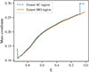 |
Fig. B.1. Evolution of the mass of the fully mixed core and semi-convective region (blue) and of the maximal overshoot region (orange). |
One could wonder why the SC region extent is very similar to the MO, despite the differences between the two schemes. The reason is that both require the local minimum of the radiative gradient in the core to be equal to the adiabatic gradient. This condition alone determines the evolution of the size of the mixed region: therefore, the extent of both SC and MO regions evolve similarly. Yet, we can note that two models with these schemes are not strictly equivalent: as the fully mixed region is larger in the MO case, the duration of the CHeB phase is extended for MO models. This, however, does not impact our work, as we sampled the parameter of space using the normalized τ variable rather than the absolute age.
Appendix C: Comparison between the Xu et al. (2013) and deBoer et al. (2017) rates for the 12C(α, γ)16O reaction
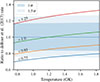 |
Fig. C.1. Ratio between the Xu et al. (2013) rates, multiplied by a given factor as done in Sect. 8, and the recommended rates from deBoer et al. (2017), with their uncertainties indicated by the blue regions. Temperatures are typical of a core of a CHeB star. To represent the deBoer et al. (2017) rates, we used the tables with update temperature resolution from Mehta et al. (2022) and accessible through Chidester et al. (2022). To compute the Xu et al. (2013) rates, we used the JINA Reaclib equation (Cyburt et al. 2010). |
Appendix D: Computing the frequencies and eigenfunctions
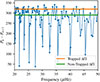 |
Fig. D.1. Consecutive period differences for a model computed with an overmixing scheme, terminated at Yc = 0.35. The asymptotic period spacing are represented by the horizontal lines, computed either in the non-trapping scenario (green) or in in the trapped scenario (orange). |
In this work, we computed the period spacing using Eq. 1, assuming the inner boundary of the g-mode cavity either to be the outer boundary of the CBM region (“trapped” scenario), or the outer boundary of the fully mixed region (“non-trapped” scenario) (see Fig. 2 for an illustration of theses boundaries for different mixing scenarios). In the following, we compare the resulting, asymptotic period spacings to the frequencies computed with an oscillation code, GYRE (Townsend & Teitler 2013). We take the peculiar case of an overmixing model that is evolved enough to have a semi-convective region around the overmixing region, with a structure that is similar to the lower left panel of Fig. 2. We present the consecutive period spacing of this model in Fig. D.1. As noted in Constantino et al. (2015), the consecutive period spacing is quite chaotic due to the complex structure of the model, which has several discontinuities notably caused by the helium sub-flashes. Thus, it is difficult to clearly determine a period spacing out of it. Yet, the period spacing computed in the trapped case is in better agreement than the one computed in the non-trapped case. We note that the model used to computed these frequencies has been smoothed compared to the ones used in the rest of the work, in order to improve the regularity of the consecutive period spacing.
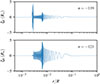 |
Fig. D.2. Horizontal displacement of dipolar modes with radial orders −119 and −121. |
Moreover, we computed the eigenfunctions of two of the modes presented in Fig. D.1, to investigate the properties of the trapped modes. We present in Fig. D.2 the horizontal displacement of the modes with radial orders −119 and −121. One can see that the mode n = −119 is mainly oscillating in the lower part of the cavity, i.e. the overshoot and the semi-convective region, and is therefore trapped in this region, while having a lower amplitude in the rest of the g-mode cavity. Oppositely, most of the modes (such as n = −121) have a small amplitude in the overshooting/semi-convection region and a large amplitude elsewhere in the g-mode cavity.
All Figures
|
Fig. 1. Period spacing distribution of the observed sample (data from Vrard et al. 2016). The uncertainties were computed following the procedure described in Appendix A. |
| In the text | |
|
Fig. 2. Brunt-Väisälä profiles of four models with different CBM schemes, which were all stopped at Yc = 0.3. We indicate the overshoot region in orange, which is fully chemically mixed with the convective core. The region in green indicates the semi-convective region, where ∇rad = ∇ad. Finally, we indicate the region over which N/r was integrated in the trapped mode scenario (red) and in the non-trapped mode scenario (purple). |
| In the text | |
|
Fig. 3. Evolution of the period spacing during the CHeB phase for models computed with (dashed line) and without taking ϵg into account in the energy equation (full line). |
| In the text | |
|
Fig. 4. Period spacing uncertainties of the sample of Vrard et al. (2016), plotted against the period spacing values of the same work. The orange line shows the linear fit that we used to simulate the uncertainties in our simulations. |
| In the text | |
|
Fig. 5. Kernel density estimations of the distributions of luminosities and effective temperature of the observed (blue) and synthetic (orange) samples, substracted by the median value of the sample. |
| In the text | |
|
Fig. 6. Distributions of the computed values of period spacing (orange) and of the observed values of period spacing (blue), for models that assume mode trapping. The lines represent the corresponding cumulative distributions. The simulated distributions were computed using a maximal overshoot scheme (upper left), a semi-convection scheme (upper right), and an overmixing scheme with αov = 0.2 (lower left) and αov = 0.5 (lower right). The represented bin uncertainties for the observations were computed following the procedure explained in Appendix A. Each bin value and associated uncertainties were normalized, i.e., divided by the total count and the bin width. |
| In the text | |
|
Fig. 7. Same as in Fig. 6, but without considering mode trapping, i.e., with period spacings being computed in the full g-mode cavity. |
| In the text | |
|
Fig. 8. Same as in Fig. 6, but for maximal overshoot and with varying 12C(α, γ)16O nuclear reaction rates. |
| In the text | |
|
Fig. 9. Evolution of the radius of the convective core (blue) and of the period spacing (orange) for a 1 M⊙, maximal-overshoot model with solar metallicity, during the CHeB phase. |
| In the text | |
|
Fig. 10. Evolution of the Brunt-Väisälä frequency profile at the location of the H-burning shell, at the very start of the CHeB phase. The lines are colored following the central helium composition: evolution goes from yellow to purple. |
| In the text | |
|
Fig. B.1. Evolution of the mass of the fully mixed core and semi-convective region (blue) and of the maximal overshoot region (orange). |
| In the text | |
|
Fig. C.1. Ratio between the Xu et al. (2013) rates, multiplied by a given factor as done in Sect. 8, and the recommended rates from deBoer et al. (2017), with their uncertainties indicated by the blue regions. Temperatures are typical of a core of a CHeB star. To represent the deBoer et al. (2017) rates, we used the tables with update temperature resolution from Mehta et al. (2022) and accessible through Chidester et al. (2022). To compute the Xu et al. (2013) rates, we used the JINA Reaclib equation (Cyburt et al. 2010). |
| In the text | |
|
Fig. D.1. Consecutive period differences for a model computed with an overmixing scheme, terminated at Yc = 0.35. The asymptotic period spacing are represented by the horizontal lines, computed either in the non-trapping scenario (green) or in in the trapped scenario (orange). |
| In the text | |
|
Fig. D.2. Horizontal displacement of dipolar modes with radial orders −119 and −121. |
| In the text | |
Current usage metrics show cumulative count of Article Views (full-text article views including HTML views, PDF and ePub downloads, according to the available data) and Abstracts Views on Vision4Press platform.
Data correspond to usage on the plateform after 2015. The current usage metrics is available 48-96 hours after online publication and is updated daily on week days.
Initial download of the metrics may take a while.