| Issue |
A&A
Volume 704, December 2025
|
|
|---|---|---|
| Article Number | A32 | |
| Number of page(s) | 12 | |
| Section | Interstellar and circumstellar matter | |
| DOI | https://doi.org/10.1051/0004-6361/202554807 | |
| Published online | 26 November 2025 | |
Edge-On Disk Study (EODS)
II. HCO+ and CO vertical stratification in the disk surrounding SSTTau042021
1
Laboratoire d’Astrophysique de Bordeaux, Université de Bordeaux, CNRS, B18N, Allée Geoffroy Saint-Hilaire,
33615
Pessac,
France
2
IRAM,
300 Rue de la Piscine,
38046
Saint Martin d’Hères,
France
3
Departamento de Física, Facultad de Ciencias, Universidad de Chile,
Av. Las Palmeras 3425,
Ñuñoa,
Santiago,
Chile
4
Institut des Sciences Moléculaires d’Orsay, CNRS, Univ. Paris-Saclay,
Orsay,
France
5
Dipartimento di Fisica e Astronomia, Università di Bologna,
Via Gobetti 93/2,
40122
Bologna,
Italy
6
Carl Sagan Center, SETI Institute,
Mountain View,
CA,
USA
7
Max-Planck-Institut für Astronomie,
Königstuhl 17,
69117
Heidelberg,
Germany
8
Konkoly Observatory, HUN-REN Research Centre for Astronomy and Earth Sciences, MTA Centre of Excellence,
Konkoly-Thege Miklós út 15-17,
1121
Budapest,
Hungary
9
Institute of Physics and Astronomy, ELTE Eötvös Loránd University,
Pázmány Péter sétány 1/A,
1117
Budapest,
Hungary
10
LUX, Observatoire de Paris, PSL Research University, CNRS, Sorbonne Universités,
92190
Meudon,
France
11
Exoplanets and Planetary Formation Group, School of Earth and Planetary Sciences, National Institute of Science Education and Research,
Jatni
752050,
Odisha,
India
12
Homi Bhabha National Institute, Training School Complex,
Anushaktinagar,
Mumbai
400094,
India
13
Astronomy Unit, School of Physics and Astronomy, Queen Mary University of London,
London
E1 4NS,
UK
14
Department of Astrophysics, Vietnam National Space Center, Vietnam Academy of Science and Technology,
18 Hoang Quoc Viet,
Cau Giay,
Hanoi,
Vietnam
15
Zentrum für Astronomie der Universität Heidelberg, Institut für Theoretische Astrophysik,
Albert-Ueberle-Str. 2,
69120
Heidelberg,
Germany
16
Academia Sinica Institute of Astronomy and Astrophysics,
11F of AS/NTU Astronomy-Mathematics Building, No.1, Sec. 4, Roosevelt Rd,
Taipei
106319,
Taiwan,
ROC
17
Institut für Theoretische Physik und Astrophysik, Christian-Albrechts-Universität zu Kiel,
Leibnizstrasse 15,
24118
Kiel,
Germany
★ Corresponding authors: This email address is being protected from spambots. You need JavaScript enabled to view it.
Received:
27
March
2025
Accepted:
1
October
2025
Abstract
Context. Edge-on disks offer a unique opportunity to directly examine their vertical structure, which provides valuable insights into planet formation processes. We investigated the dust properties as well as the CO and HCO+ gas properties in the edge-on disk surrounding the T Tauri star 2MASS J04202144+281349 (SSTTau042021).
Aims. We estimated the radial and vertical temperature and density profile for the gas and the dust.
Methods. We used ALMA archival data of CO isotopologs and continuum emission at 2, 1.3, and 0.9 mm together with new NOEMA HCO+ 3-2 observations. We retrieved the gas and dust disk properties using the tomographic method and the DISKFIT model.
Results. The vertical CO emission appears to be very extended and partly traces the H2 wind observed by JWST. The C18O, 13CO, and HCO+ emission characterize the bulk of the molecular layer. The dust and gas have midplane temperatures of ∼7-11 K. The temperature of the molecular layer (derived from 13CO and HCO+) is on the order of 16 K. Because HCO+ 3-2 is thermalized, we derived a lower limit for the H2 volume density of ∼3 × 106 cm−3 at a radius of 100-200 au between one and two scale heights. The atmosphere temperature of the CO gas is ∼31 K at a radius of 100 au. We directly observed CO and HCO+ gas in the midplane beyond the dust outer radius (≥300 au). The gas plus dust disk mass estimated up to a radius of 300 au is on the order of 4.6 × 10⁻² M⊙.
Conclusions. The favorable disk inclination allows us to present the first quantitative evidence for vertical molecular stratification with a direct observation of CO and HCO+ gas in the midplane. We estimate a temperature profile with a temperature of 7-11 K near the midplane and of 15-20 K in the dense part of the molecular layer up to ∼35 K above the midplane.
Key words: protoplanetary disks / astrochemistry
© The Authors 2025
 Open Access article, published by EDP Sciences, under the terms of the Creative Commons Attribution License (https://creativecommons.org/licenses/by/4.0), which permits unrestricted use, distribution, and reproduction in any medium, provided the original work is properly cited.
This article is published in open access under the Subscribe to Open model. This email address is being protected from spambots. You need JavaScript enabled to view it. to support open access publication.
1 Introduction
Gas-rich protoplanetary disks are natural laboratories in which we can study planet formation mechanisms. Their composition and structure provide key insights into how planets assemble from gas and dust under varying physical conditions.
Current large millimetre and submillimetre arrays, such as the Atacama large millimetre/submillimetre array (ALMA) and the northern extended millimetre array (NOEMA) enable us to study their gas and dust properties with sufficient angular resolution and sensitivity to start investigations on planet-forming regions. For instance, the ALMA large program called disk substructures at high angular resolution project (DSHARP) observed rings and spirals in dust disks that may be caused by active planet formation (Andrews et al. 2018).
The ALMA large program MAPS (molecules with ALMA at planet-forming scales) provided a significant contribution to the understanding of the gas phase by observing five large inclined disks around TTauri and Herbig Ae stars at a high resolution. This delivered unprecedented insights into the gas temperature, density, and composition. Key molecules such as HCO+, CN, HCN, HNC, CS, and N2H+ were observed (Guzmán et al. 2021). Of these, HCO+ plays a crucial role because it provides invaluable insights into the ionization structure of disks, especially in regions in which other tracers become less reliable (Aikawa et al. 2021). Models suggest that HCO+ is probably emitted from a region similar to CO, closer to the disk midplane (Aikawa et al. 2002).
Accurate CO observations allow us to retrieve the kinetic gas temperature because the first rotational lines are thermalized and optically thick (Dartois et al. 2003; Franceschi et al. 2024). In five disks, a parametric approach was used to derive the radial and vertical temperature profiles (Law et al. 2021) and a more complex approach that used a thermo-chemical model (Zhang et al. 2021). The comparison shows that both approaches provide similar thermal structures in the temperature range of 15-40 K (Zhang et al. 2021). Several attempts were made recently to improve these methods (e.g. Paneque-Carreño et al. 2023). These retrieval methods require that an emitting surface or thin layer is identified, but their performance would degrade for geometrically thick layers that are probed by optically thin transition because of the combined effects of the density, temperature, and velocity gradients along the line of sight, which hamper the identification of the sampled (r, z) locations.
Edge-on disks are not affected by this limitation because the disk radii appear as a straight line in the velocity-position diagram that provides a tomographically reconstructed distribution (TRD) of the disk structure by averaging the molecular emission along each radius (Dutrey et al. 2017). When the observed line is optically thick and thermalized, such as the 12CO lines, the gas temperature can be derived directly (Dutrey et al. 2017; Pinte et al. 2018; Flores et al. 2021). For an optically thinner molecular transition, the vertical distribution of the observed molecule is estimated directly.
Finally, ALMA observations of dust disks have also offered accurate evidence of dust settling at millimeter wavelengths (e.g. Guilloteau et al. 2016; Villenave et al. 2020, 2022; Franceschi et al. 2023), but the molecular stratification of the disk remains largely unexplored. We analyze new NOEMA observations of HCO+ 3-2 together with ALMA archival CO and continuum data of the disk orbiting 2MASS J04202144+2813491 (hereafter SSTTau042021). This is a Class II TTauri star with a mass of 0.27 M⊙ (Simon et al. 2019) that is located in the Taurus cloud at a distance of ∼160 pc. The dust disk is observed very close to edge-on (inclination >85°), is settled, and has an outer radius of ∼350 au, while the CO disk extends up to ∼700 au (Villenave et al. 2020). More recently, James Webb Space Telescope (JWST) observations by Arulanantham et al. (2024) and Duchêne et al. (2024) revealed extended vertical emission from H2 rotational transitions with an X shape that likely arises from an MHD disk wind that extends to about 200 au above the midplane (see also Fig. 3).
ALMA and NOEMA continuum and line observations.
2 Observations and data reduction
2.1 Observations
We used ALMA archival data for CO isotopologs and continuum at related frequencies, as well as for the 145 GHz continuum, and observed the HCO+ 3-2 line with the NOEMA interferometer. Table 1 presents the main observational characteristics of the data.
NOEMA. The new long baselines (up to 1600 m) were used to observe SSTTau042021 in HCO+ 3-2 and in continuum in January 2023 (project W22BC). These data were completed by observations in C configuration (baseline range of 16-350 m) in November 2024 (project S24AT), to provide more sensitivity to extended emission. The data were calibrated using the standard CLIC pipeline.
ALMA. Observations were performed in projects 2016.1.00771.S for the 12CO, 13 CO, and C18O 2-1 lines and the continuum at 230 GHz and 2016.1.00460.S for the 12CO 3-2 transition and the continuum at 345 GHz and 150 GHz (Table 1). Project 2016.1.00771.S was observed in configuration C40-6, with baselines ranging from 15 to 1800 meters, and project 2016.1.00460.S was observed in configuration C40-4, with baselines from 15 to 704 meters. The data were calibrated with the standard ALMA pipeline (see Simon et al. 2019, for details of the CO line data) and exported in UVFITS format for further use.
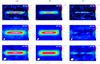 |
Fig. 1 Continuum observations. Left column (a): observation. Middle column (b): best model. Right column (c): difference (observation - model). The rms noise levels reach 0.1 K at 146 GHz, 6.55 × 10⁻³ K at 225 GHz, and 1.33 × 10⁻² K at 333 GHz. The peaks of the residuals correspond to 5.2σ at 146 GHz, 11.8σ at 225 GHz, and 8.7σ at 3 33 GHz. |
2.2 Data reduction
Proper motions. ALMA and NOEMA sampled four different epochs between October 2016 and November 2024. This allowed us to measure the proper motion of the source. The values μα = 14.6 ± 2.2 and μδ = −22.2 ± 2.0 mas/yr are consistent with those of the nearby T Tau stars. All data were recentered to the source position RA = 04:20:21.4568 and Dec 28:13:48.99 at epoch 2016.0 for easier reference to GAIA.
Imaging. All imaging was performed using IMAGER1. For all the data, the images were obtained with natural weighting, and were rotated by −73.5° as required to bring the disk rotation axis along the Y-axis.
The left panels of Fig. 1 show the images from ALMA at 146, 224.4, and 333 GHz. The source continuum structure is highly resolved in one direction, which precluded the use of self-calibration. The continuum images are thus limited by the dynamic range, but the spectral line data are limited by thermal noise. Figure A.1 shows 12CO 2-1, 12CO 3-2, 13 CO 2-1, and C18O 2-1 with the HCO+ 3-2 channel maps. Integrated area maps of CO 2-1 and HCO+ 3-2 are shown in Fig. 2. The 12CO maps show that emission is absent in some channels (from 7.11 to 8.07 km/s for the 2-1 line, and from 7.04 to 7.89 km/s for the 3-2 line). This results from contamination by CO emission from clouds along the line of sight. As a result, the CO moment maps (Fig. 2) exhibit an asymmetry between the blue- and redshifted sides. At the maximum recoverable scale (MRS; see Table 1), only little flux is lost (less than 10%). The recovered flux is confused with the molecular cloud in CO, however. Figure 3 is a montage showing the superimposition of the CO and HCO+ intensity maps with the H2 S(2) emission from the JWST.
3 Tomographies
A tomography is a two-dimensional image of the gas temperature as a function of radius and height. The image is obtained by averaging the observed intensity along the lines of the positionvelocity (PV) diagram. Because the disk rotates, each of these lines corresponds to a specific radius within the disk. This geometric characteristic allows us to directly reconstruct the twodimensional luminosity distribution (Dutrey et al. 2017). The resulting tomographic image has a constant linear resolution with height above the disk midplane, while the resolution varies with radius. It decreases at larger radii because the Keplerian shear relative to local line width decreases as well (Dutrey et al. 2017).
The TRD based on the mean temperature for each radius is presented in the left panels of Fig. 4. The TRD reveals some top-bottom asymmetries that likely arise because the disk is not observed perfectly edge-on (Dutrey et al. 2017). Moreover, the 12 CO TRD was produced using all velocity channels, and it is thus affected by the confusion with the molecular clouds. This makes an interpretation of the TRD more difficult (although this confusion is limited to areas of integration along the radii).
The TRDs are efficient for a direct visualization of the vertical stratification, but the radial resolution varies because the ratio of Keplerian shear to the intrinsic local line width decreases with radius. A direct interpretation of the TRD is also only possible for optically thick thermalized lines. Radiative transfer modeling is thus required to properly constrain the gas properties.
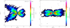 |
Fig. 2 Integrated-intensity map of 12CO 2-1 (left, clipped at 22 mJy/beam km/s), and integrated-intensity map of HCO+ 3-2 (right, clipped at 8 mJy/beam km/s). The maps are rotated by −73.5°. The contours are defined from 0 to 0.1 Jy/beam km/s in steps of 0.01 Jy/beam km/s, i.e., 3.36σ for the 12CO 2-1 map, and from 0 to 0.5 Jy/beam km/s in steps of 0.02 Jy/beam km/s , i.e., 2.30σ for the HCO+ 3-2 map. |
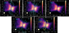 |
Fig. 3 Montage of JWST and interferometric data for SSTTau042021. MIRI MRS images from JWST reveal H2 S(2) emission at 12.278-μm (Arulanantham et al. 2024). The white contours indicate the mid-infrared scattered-light continuum at 12.2-μm, and the dashed white line marks the rotation axis of the disk at PA = 73.5°. In archival ALMA data and new NOEMA observations, the cyan contours show molecular emission lines of HCO+ 3—2, 13CO 2—1, C18O 2-1, 12CO 2-1, and 12CO 3-2, and the yellow contours represent the 0.85 mm continuum emission at 1 mJy/beam. The beige circles in the bottom left corner of each panel represent the average theoretical FWHM of the PSF for JWST data, calculated from the relation reported by Law et al. (2023), and the beam of the molecular line emission is shown as a cyan ellipse in the top right corner of each panel. The contours for HCO+ (3-2) range from 0.02 to 0.2 Jy/beam km/s with a step of 0.02 Jy/beam km/s, i.e., 2.5 œ; for 13CO (2-1), they range from 0.02 to 0.08 Jy/beam km/s with a step of 0.01 Jy/beam km/s, i.e., 3.5 œ; for C18CO (2-1), they range from 0.008 to 0.016 Jy/beam km/s with a step of 0.008 Jy/beam km/s, i.e., 3.5 œ; for 12CO (2-1), from 0.01 to 0.08 Jy/beam km/s with a step of 0.02 Jy/beam km/s, i.e., 6 œ; and for 12CO (3-2), from 0.06 to 0.8 Jy/beam km/s with a step of 0.06 Jy/beam km/s, i.e., 4.2σ. |
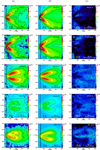 |
Fig. 4 From top to bottom: TRD of 12CO 2-1, 12CO 3-2, 13CO 2-1, C18O 2-1 and HCO+ 3-2: (a) TRD of the observations. (b) TRD of the final result of the models. (c) Difference between the observations and model TRD. For 12CO (2-1), the residuals range from −2 to 2 K, while for the 12CO (3-2) transition, they extend from −3 to 2 K. In the case of 13CO (2-1), the differences are between 0 and 2 K. For C18O (2-1), the deviations range from −1 to 2 K, and for HCO+ (3-2), they span from −1 to 3 K. The vertical black line represents the effective resolution, and the two error bars show the widening of the beam as a function of radius caused by the TRD method. The contours are defined from 4 K to 20 K in steps of 2 K for the observational and model maps, and from −3 K to 3 K in steps of 1 K for the residual maps. |
Continuum-fit parameters and results.
4 Modeling
The limited quality of the CO data due to CO cloud confusion and the very short integration time precludes the use of a complex modeling approach. We therefore adopted a parametric radiative transfer code, the DiskFit tool (Piétu et al. 2007), to estimate the basic physical parameters (Tables 2 and 3). The DiskFit adjustment was made by comparing the predicted visibilities to the observations in the Fourier plane.
The vertical gas density distribution follows a Gaussian profile with a scale height H(r) defined by n(r, z) = n(r, 0) exp(−(z∕H(r))2). The scale height, molecular surface densities, and rotational or dust temperatures are defined as power laws with radius, the disk size being truncated by sharp inner and outer radii.
The vertical temperature profile can be taken as isothermal, or a gradient mimicked by parametric laws can be assumed (routinely used for disks e.g. Law et al. 2021). We used the specific prescription of Dutrey et al. (2017). We used the so-called LTE mode in DiskFit, which provides the excitation temperature for the observed lines. The local velocity dispersion (thermal and turbulent motions) was assumed to be constant over the disk. The details are given in Appendix B.
4.1 Continuum data
We analyzed the continuum data assuming that the dust absorption coefficient is a power law of the frequency with a value 0.052 cm2 g−1 at 345 GHz (including a gas-to-dust ratio of 100, Beckwith et al. 1990). The dust emissivity index β was also a free parameter in the minimization process and converged toward a value of 0.6. We derived the geometrical parameters and then minimized the dust surface density ΣD (r) and temperature TD (r). Because the dust emission is concentrated around the disk midplane, we assumed a simple radial power law with a vertically isothermal profile. The datasets were first independently minimized (the same geometrical parameters were found for the three datasets). The dust scale height Hd(r) was derived from 220 and 330 GHz data alone. We then minimized the three ALMA datasets (continuum at 146, 255, and 333 GHz) together, and Table 2 presents the resulting best-fit model. At 146 GHz, the residuals reach about 0.1 K, and they drop to 6.6 × 10⁻³ K at 225 GHz and 1.3 × 10⁻² K at 333 GHz. The higher residuals at 146 GHz (see Fig. 1) may indicate a more settled dust layer of larger grains that are not well represented at the other frequencies.
4.2 Molecular lines
In the analysis of the 12CO 2-1 and 3-2 lines, we ignored channels that were contaminated by cloud emission (see Sec. 2.2 and Fig. A.1). We modeled the line data with and without continuum subtraction and obtained similar results for geometrical and velocity parameters, as well as for the temperature law. The final fit was performed with the continuum, using the best-fit dust parameters from Table 2. Because molecular depletion induced by freeze-out may occur in the disk midplane owing to the very low temperatures derived from the dust, we also verified that the fitted gas temperature law was similar regardless of freeze-out (following two criteria, one criterion for the gas temperature T(r, z), and a second criterion for the H2 column density; see Appendix B for details). Finally, because the signal-to-noise ratio was low, we analyzed the C18O 2-1 emission assuming the 13CO parameters and only fit the surface density at 100 au.
Table 3 presents the best model parameters for the five lines 12CO 2-1 and 3-2, 13CO 2-1, C18O 2-1, and HCO+ 3-2. Figure 4 presents the TRD of the observations (left panels), the TRD of the best-fit DiskFit models (middle panels), and their differences (right panels: observation TRD minus model TRD). Figure B.1 shows the two-dimensional density and temperature distributions derived for 12CO, 13CO, HCO+, and the dust.
5 Discussion
5.1 Dust disk
The best-fit model (Table 2) shows that the dust disk has no cavity, is large, and is relatively cold, with a radially constant temperature of ∼ 10 K. Millimeter observations are sensitive to large grains, which might be colder than the smaller grains (Gavino et al. 2021), and this low temperature is therefore not surprising. Within the error bars, the dust temperature is also about the same as the gas temperature (8-10 K; Table 3). We searched for possible variations in β with radius (as observed by Guilloteau et al. 2011; Testi et al. 2014; Pérez et al. 2012), and we found that the best fit is given for a constant value of β.
The right panel of Fig. 1 shows the difference map between the observations and the best models for the three frequencies. The model appears to be more centrally peaked than the observations, that is, it is less optically thick, which is unusual for observations of an edge-on disk. Nevertheless, because this part of the disk is strongly diluted by the beam, these results need to be taken with caution. Moreover, because we were not able to self-calibrate the data, some low-level features seen around the disk in the left panels (particularly at 1 mm) may be due to uncorrected small phase errors. Panel c in Fig. 1 suggests evidences for a gap at a radius of ∼70-150 au (on both sides), however, particularly at 150 and 330 GHz. This feature is seen neither in CO nor in HCO+, however. More molecular data are needed to investigate the origin of this potential gap.
The power-law index of the surface density (given by ΣD (r) = ΣD0(r/100au)−p) p is very flat (0.5 ± 0.2). Boehler et al. (2013) showed that when large grains settle onto the midplane, the fit exponent p can become negative. The derived value suggests an intermediate case with moderate settling, perhaps because SSTTau042021 is young, like the Butterfly Class I system (Gräfe et al. 2013), or possibly also because settling is less efficient because the stellar mass is very low (0.27 M⊙).
By integrating the dust surface density, we estimated the total disk mass (gas plus dust) to be ∼4.6 × 10⁻² M⊙ (assuming a gas-to-dust ratio of 100). This value is consistent with the lower limit reported by Villenave et al. (2020).
Best-fit models for the molecular lines.
5.2 A disk wind traced by CO?
Figures A.1, 3, and 4 show that the CO emission is larger in the vertical direction than the emission of the other molecules. Figure 5 presents two specific channels of the 12CO 2-1 emission that are less affected by the foreground cloud that is superimposed on the H2 S(2) integrated area map from (Arulanantham et al. 2024). Fig. 5 shows that the two large tori of CO gas encircle the H2 S(2) disk wind that is launched from the top and bottom of the disk atmosphere, at above ∼4 scale heights.
This nested morphology of the disk molecular winds has been predicted theoretically (Wang et al. 2019) and was recently confirmed by the JWST observations of several edge-on disks by Pascucci et al. (2025). Molecules such as CO can be launched by the wind from the upper molecular disk layer high up into the highly FUV-irradiated disk atmosphere, where they are gradually dissociated and cannot be easily produced again via ion-molecule reactions because the densities are low and the corresponding collisional timescales are short (Panoglou et al. 2012). The vertical distribution of CO appears to be more confined to the disk than the H2 IR emission, either (1) because ALMA is less sensitive at submillimeter wavelengths than JWST at mid-IR wavelengths and/or (2) because the UV dissociation of the CO gas is more efficient, despite its self-shielding and mutual shielding by the H2, as CO molecules are much less abundant than H2 molecules (van Dishoeck & Black 1988).
On the other hand, there is no significant signature of such an extended morphology in the 13CO, C18O, and HCO+ emission, as shown in Figs. A.1 and 3. This would be expected in a disk-wind interpretation because the column densities of these molecules in the disk atmosphere from which the disk wind launches are insufficient. The relative faintness in CO 3-2 may also indicate a low density or low temperature there.
We note that in our DiskFit analysis, we excluded velocity channels contaminated by the cloud emission (as indicated by the crosses in Fig. A.1), which cover a substantial part of the putative disk-wind region. Thus, this disk wind is therefore not expected to affect our determination of the disk parameters. The main issue affecting the interpretation is contamination from the surrounding molecular cloud and not the disk wind itself.
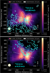 |
Fig. 5 As in Figure 3, overlay of the JWST image from Arulanantham et al. (2024) with contours of the 12CO (2-1) channel maps at 6.80 km/s and 8.23 km/s illustrating the large vertical extent around the H2 emission. The contours are in steps of 3.4σ and range from 10 to 40 mJy beam−1. |
5.3 Gas temperature
Table 3 and Figs. 4, B.1 present the results of the best models for the observed molecules. The results from 12CO may be partly corrupted by the confusion with the CO clouds and that due to beam dilution. Our results are not significant below a radius of −50 au.
At a radius of about 50-250 au, that is, in the densest disk area, we found that the atmospheric gas temperature is essentially higher for 12CO than for 13CO. This is expected because the bulk of the 13CO gas is located at a lower altitude than the much more optically thick 12CO emission, which reflects more the whole extent of the molecular gas. With or without freeze-out in the disk midplane, we always derived a temperature for the molecular layer of 15-20 K, which is very close to the freeze-out temperature of CO.
It is harder to determine the midplane temperature because it depends a priori on the assumed shape of the vertical temperature profile, and it may also be affected by the continuum emission. All models converged toward low midplane temperature values of about 9 K at 100 au.
This temperature increased to 25 K in the upper layers. Similar temperatures were also observed for the edge-on disk around the Flying Saucer by Dutrey et al. (2017). Our values are lower than those obtained by Flores et al. (2021) for the brighter source Oph1631 that is also seen edge-on. They found about 20 K at a radius <200 au near the midplane, and a temperature of −30 K for the upper layer, with an almost vertically isothermal profile beyond a radius of 200 au.
The (excitation) temperature distributions derived from HCO+ 3-2 and 13CO 2-1 closely agree. Since the later transition is thermalized, this implies the HCO+ 3-2 line is thermalized as well. This sets a lower limit to the density in the emitting region.
We tried to assess the impact of our simple mathematical prescription on the results (Appendix B). The best-fit model (which has a value of the exponent δ≃ 2.5-3 that controls the steepness) suggests that the transition of the temperature from the midplane to the bulk of the molecular emission region, which is at lower altitude for 13CO and HCO+ than for 12CO, is very steep.
5.4 Molecular distribution
In the midplane, the TRD (Fig. 2, panel a) suggests an absence of emission. This may be a result of the lower gas temperature in the midplane, as found for HD 163296 by Dullemond et al. (2020). Our extrapolated midplane temperature is much lower than the 18 K found in the above case, however, so that we also expect molecules to be underabundant at these very low temperatures due to freeze-out on cold grains (Gavino et al. 2021; Ruaud & Gorti 2019). We handled this effect using models with a complete freeze-out of molecules in cold and UV-shielded regions (see Appendix B and Fig. B.1 for details). This improved the fits, particularly for the CO (2-1) model, by reducing the residuals near the midplane (see Fig. B.2). This suggests that this depletion is indeed present. Figure B.2 shows that without depletion in the model, the residuals near the disk midplane increase by approximately 1K. Although this effect is less pronounced in the residual maps of the other lines, the data quality for these transitions is insufficient to clearly confirm this behavior. Nevertheless, since the effect is clearly observed for 12CO, it is more consistent to assume that a similar depletion is present for all lines.
Several studies have provided direct evidence that molecular gas extends beyond the outer dust disk radius in protoplanetary disks. For instance, Panic et al. (2009) and Cleeves et al. (2016) observed 12CO emission in the IM Lup disk that extended to 970 au, while the millimeter continuum emission was truncated at 313 au. Although the signal-to-noise ratio is lower, our observations also indicate cold molecular gas beyond the outer edge of the dust disk. The DiskFit analysis clearly confirms this, with much larger outer radii for CO and HCO+ than for dust.
In addition, the TRD of the residuals for 13CO and C18O seem to exhibit some additional emission beyond the outer dust radius (at > 350-400 au). This suggests an additional gas component that is not represented by our simple power disk model.
Vertically, the molecular extents of the HCO+ and 13CO emission appear to be relatively similar. The TRD of the differences (Fig. 4, panel c) shows for 13CO that above and below the midplane, the model also exhibits excess emission that remains difficult to quantify, however, because of the limitations imposed by the data quality. We note, however, that the apparent height of HCO+ is about 30% larger than that of 13CO. The molecular scale heights, 24-30 au at 100 au, should not be confused with the hydrostatic equilibrium scale height, about 15 au, given the midplane temperature of 10 K, nor with the dust scale height, whose value (11 au) suggests moderate settling. This suggests that HCO+, the most abundant molecular ion in disks, is essentially formed at an intermediate altitude in the disk (at about 2 hydrostatic scale heights). This agrees with the work from van’t Hoff et al. (2017), who used detailed physical and chemical modeling to demonstrate that HCO+ is predominantly formed in the warm molecular layer of the disk, specifically, at intermediate heights above the midplane.
Finally, because HCO+ 3-2 seems to be thermalized, we can determine a lower value for the local H2 density at a radius of 100 au, which should be significantly higher than the critical collision density of the 3-2 rotational HCO+ transition −2.2 × 106 cm−3 (Denis-Alpizar et al. 2020). At the scale height at which the emission is visible, this translates into −108 cm−3 in the midplane. This value is consistent with the density extrapolated from dust emission.
6 Summary
CO clouds complicate the analysis, but the 12CO emission is vertically extended. It partly traces the H2 wind observed by JWST;
HCO+, C18O, and 13CO trace the bulk of the molecular layer;
The gas and dust midplane temperatures are ~8-12 K, the molecular layer temperature (from 13CO and HCO+) is ~16K, and the atmospheric temperature of the CO gas is ~31 K at 100 au;
HCO+ 3-2 is thermalized, which sets a lower limit for the H2 density of ~2.2 × 106 cm−3 at 100-200 au;
The CO and HCO+ TRD residuals suggest that some gas is in the midplane beyond the outer dust radius (≥300 au).
Acknowledgements
This work is based on observations carried out under projects number W22BC & S24AT with the IRAM NOEMA Interferometer. IRAM is supported by INSU/CNRS (France), MPG (Germany) and IGN (Spain). This work was supported by the Thematic ActionS “Programme National de Physique Stellaire” (PNPS) and “Physique et Chimie du Milieu Interstellaire” (PCMI) of INSU Programme National “Astro”, with contributions from CNRS Physique & CNRS Chimie, CEA, and CNES. This research made use of the SIMBAD database, operated at the CDS, Strasbourg, France. Y.W.T. acknowledges support through NSTC grant 111-2112-M-001-064- and 112-2112-M-001-066. This paper makes use of the following ALMA data: 2016.1.00771.S and 2016.1.00460.S. ALMA is a partnership of ESO (representing its member states), NSF (USA) and NINS (Japan), together with NRC (Canada), NSTC and ASIAA (Taiwan), and KASI (Republic of Korea), in cooperation with the Republic of Chile. The Joint ALMA Observatory is operated by ESO, AUI/NRAO and NAOJ. This work was also supported by the NKFIH NKKP grant ADVANCED 149943 and the NKFIH excellence grant TKP2021-NKTA-64. N. T. Phuong acknowledges support from Vietnam Academy of Science and Technology under grant number VAST 08.02/25-26.
References
- Aikawa, Y., van Zadelhoff, G. J., van Dishoeck, E. F., & Herbst, E. 2002, A&A, 386, 622 [NASA ADS] [CrossRef] [EDP Sciences] [Google Scholar]
- Aikawa, Y., Cataldi, G., Yamato, Y., et al. 2021, ApJS, 257, 13 [NASA ADS] [CrossRef] [Google Scholar]
- Andrews, S. M., Huang, J., Pérez, L. M., et al. 2018, ApJ, 869, L41 [NASA ADS] [CrossRef] [Google Scholar]
- Arulanantham, N., McClure, M. K., Pontoppidan, K., et al. 2024, ApJ, 965, L13 [NASA ADS] [CrossRef] [Google Scholar]
- Beckwith, S. V. W., Sargent, A. I., Chini, R. S., & Guesten, R. 1990, AJ, 99, 924 [Google Scholar]
- Boehler, Y., Dutrey, A., Guilloteau, S., & Piétu, V. 2013, MNRAS, 431, 1573 [Google Scholar]
- Cleeves, L. I., Öberg, K. I., Wilner, D. J., et al. 2016, ApJ, 832, 110 [Google Scholar]
- Dartois, E., Dutrey, A., & Guilloteau, S. 2003, A&A, 399, 773 [CrossRef] [EDP Sciences] [Google Scholar]
- Denis-Alpizar, O., Stoecklin, T., Dutrey, A., & Guilloteau, S. 2020, MNRAS, 497, 4276 [Google Scholar]
- Duchêne, G., Ménard, F., Stapelfeldt, K. R., et al. 2024, AJ, 167, 77 [CrossRef] [Google Scholar]
- Dullemond, C. P., Isella, A., Andrews, S. M., Skobleva, I., & Dzyurkevich, N. 2020, A&A, 633, A137 [EDP Sciences] [Google Scholar]
- Dutrey, A., Guilloteau, S., Piétu, V., et al. 2017, A&A, 607, A130 [CrossRef] [EDP Sciences] [Google Scholar]
- Flores, C., Duchêne, G., Wolff, S., et al. 2021, AJ, 161, 239 [NASA ADS] [CrossRef] [Google Scholar]
- Franceschi, R., Birnstiel, T., Henning, T., & Sharma, A. 2023, A&A, 671, A125 [NASA ADS] [CrossRef] [EDP Sciences] [Google Scholar]
- Franceschi, R., Henning, T., Smirnov-Pinchukov, G. V., et al. 2024, A&A, 687, A174 [NASA ADS] [CrossRef] [EDP Sciences] [Google Scholar]
- Galloway-Sprietsma, M., Bae, J., Izquierdo, A. F., et al. 2025, ApJ, 984, L10 [Google Scholar]
- Gavino, S., Dutrey, A., Wakelam, V., et al. 2021, A&A, 654, A65 [NASA ADS] [CrossRef] [EDP Sciences] [Google Scholar]
- Gräfe, C., Wolf, S., Guilloteau, S., et al. 2013, A&A, 553, A69 [NASA ADS] [CrossRef] [EDP Sciences] [Google Scholar]
- Guilloteau, S., Dutrey, A., Piétu, V., & Boehler, Y. 2011, A&A, 529, A105 [NASA ADS] [CrossRef] [EDP Sciences] [Google Scholar]
- Guilloteau, S., Piétu, V., Chapillon, E., et al. 2016, A&A, 586, L1 [NASA ADS] [CrossRef] [EDP Sciences] [Google Scholar]
- Guzmán, V. V., Bergner, J. B., Law, C. J., et al. 2021, ApJS, 257, 6 [CrossRef] [Google Scholar]
- Law, C. J., Teague, R., Loomis, R. A., et al. 2021, ApJS, 257, 4 [NASA ADS] [CrossRef] [Google Scholar]
- Law, C. J., Booth, A. S., & Öberg, K. I. 2023, ApJ, 952, L19 [NASA ADS] [CrossRef] [Google Scholar]
- Paneque-Carreño, T., Miotello, A., van Dishoeck, E. F., et al. 2023, A&A, 669, A126 [NASA ADS] [CrossRef] [EDP Sciences] [Google Scholar]
- Panic, O., Hogerheijde, M. R., Wilner, D., & Qi, C. 2009, A&A, 501, 269 [NASA ADS] [CrossRef] [EDP Sciences] [Google Scholar]
- Panoglou, D., Cabrit, S., Pineau Des Forêts, G., et al. 2012, A&A, 538, A2 [CrossRef] [EDP Sciences] [Google Scholar]
- Pascucci, I., Beck, T. L., Cabrit, S., et al. 2025, Nat. Astron., 9, 81 [Google Scholar]
- Pérez, L. M., Carpenter, J. M., Chandler, C. J., et al. 2012, ApJ, 760, L17 [CrossRef] [Google Scholar]
- Piétu, V., Dutrey, A., & Guilloteau, S. 2007, A&A, 467, 163 [Google Scholar]
- Pinte, C., Ménard, F., Duchêne, G., et al. 2018, A&A, 609, A47 [NASA ADS] [CrossRef] [EDP Sciences] [Google Scholar]
- Qi, C., Öberg, K. I., Wilner, D. J., et al. 2013, Science, 341, 630 [Google Scholar]
- Ruaud, M., & Gorti, U. 2019, ApJ, 885, 146 [Google Scholar]
- Simon, M., Guilloteau, S., Beck, T. L., et al. 2019, ApJ, 884, 42 [NASA ADS] [CrossRef] [Google Scholar]
- Testi, L., Birnstiel, T., Ricci, L., et al. 2014, in Protostars and Planets VI, eds. H. Beuther, R. S. Klessen, C. P. Dullemond, & T. Henning, 339 [Google Scholar]
- van Dishoeck, E. F., & Black, J. H. 1988, ApJ, 334, 771 [Google Scholar]
- van ’t Hoff, M. L. R., Walsh, C., Kama, M., Facchini, S., & van Dishoeck, E. F. 2017, A&A, 599, A101 [CrossRef] [EDP Sciences] [Google Scholar]
- Villenave, M., Ménard, F., Dent, W. R. F., et al. 2020, A&A, 642, A164 [EDP Sciences] [Google Scholar]
- Villenave, M., Stapelfeldt, K. R., Duchêne, G., et al. 2022, ApJ, 930, 11 [NASA ADS] [CrossRef] [Google Scholar]
- Wang, L., Bai, X.-N., & Goodman, J. 2019, ApJ, 874, 90 [Google Scholar]
- Zhang, K., Booth, A. S., Law, C. J., et al. 2021, ApJS, 257, 5 [NASA ADS] [CrossRef] [Google Scholar]
Appendix A Observations
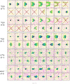 |
Fig. A.1 Velocity channel maps from top to bottom: for 12CO 2-1, 3-2, 13CO 2-1, C18O 2-1 and HCO+ 3-2. The channels corrupted by the CO clouds along the line of sight are marked with a red cross. These channels were not used in the DiskFit analysis. All the maps are rotated by −73.5°. The contours are defined as follows: from 3 to 12 K in steps of 3 K (i.e., 3.6σ) for the 12CO 2-1, 3.3σ for 12CO 3-2, and 3.6σ for 13CO 2-1; from 2 to 6 K in steps of 2 K (i.e., 3.2σ) for C18O 2-1; and from 3 to 9 K in steps of 3 K (i.e., 3.3σ) for HCO+ 3-2. |
Appendix B Modeling
B.1 Basic parameters
In Diskfit (Piétu et al. 2007), a disk is characterized by several parameters, for which error bars can be derived. These parameters include the atmospheric and mid-plane temperatures (Tatm, Tmid, the scale height (H(r)), the surface density (Σ(r)), the inner and outer radius (Rin,Rout), disk velocity, disk orientation and inclination, and stellar mass. For the final minimization, we fix the pivot R0 at 100 au to maximize the sensitivity. The version of the model we used operates under the assumption of LTE conditions and azimuthal symmetry. For lines which are not thermalized, the derived temperature thus corresponds to the line excitation temperature. The vertical distribution of the matter is assumed to follow a Gaussian profile, as n(r, z) = n(r, z = 0)exp(−(z/H(r))2), where the scale height H(r) varies as a power law with radius. Note that with such a definition of scale heights, the hydrostatic scale height in the disk mid-plane would be H = √2Cs/ΩK where Cs is the isothermal sound speed and Ωk the Keplerian angular velocity, a factor √2 larger than the alternate definition used in some other works.
The local velocity dispersion δV, which encompasses thermal and turbulent motions on scales smaller than the beam size, is assumed to be radially constant, as the data have insufficient sensitivity to reveal possible spatial variations. To find the best model by minimization, Diskfit proceeds by comparison in the uv plane in order to reduce the non linear deconvolution effects.
B.2 Depletion Zone
To constrain the presence of gas onto the mid-plane, the final runs were performed including a depletion factor near the midplane, with two criteria, one onto the gas temperature T(r, z) and a second onto the H2 column density from the current height to the outside,  .
.
Molecules are only present if T(r, z) > Tdep (with accounts for molecules sticking on grains at low temperatures) or Σz(r, z) < Σdep (to account for photo-desorption from dust when sufficient interstellar UV radiation penetrates).
Following the results reported by Qi et al. (2013), we assumed a depletion temperature of 17.5 K for all our molecules. We found similar values for Σdep ≈ 3.6 1022 cm−2 for CO and 13CO, while for HCO+, Σdep=8.7 ± 0.2 1022 cm−2 suggests that HCO+ extends closer to the mid-plane than CO.
The better fits obtained with depletion is illustrated in Fig. B.2 which shows the residual TRD of 12CO with and without depletion zone. For HCO+, which actually has a smaller depletion area (see Fig. B.1), the difference is less significant, as for 13 CO and C18O because of their limited opacities.
B.3 Temperature profile
Temperature radial and vertical profiles are modeled following Dartois et al. (2003) and Dutrey et al. (2017). The disk atmosphere temperature is given by:
 (B.1)
(B.1)
while the mid-plane temperature corresponds to:
 (B.2)
(B.2)
In between, for an altitude of z < zqH(r), the temperature is defined by:
 (B.3)
(B.3)
The atmospheric temperature was minimized together with the values of zq and δ which controls the position and sharpness (δ) of the vertical temperature gradient. We did several checks to determine their impact on the fit. The best fit models systematically correspond to a very steep value of δ ≃ 2.5-3, but simultaneous adjustment of δ and zq were not possible. We finally opted for δ = 2.5 and found zq ~ 1.2, indicating that the steep gradient is at about 0.3 H(r). Here, H(r) is the apparent scale height of the molecule distributions: the hydrostatic scale height derived from the mid-plane temperature is about a factor 2 lower.
We tested the robustness of our results by modifying the functional form of the temperature profile and replacing the cosine dependence with a sine function. This alternative prescription leads to nearly identical results in the minimization procedure, both in terms of temperature structure and line emission fits.
 (B.4)
(B.4)
Best fit models for 13CO 2-1 assuming Eq. B.4
This consistency demonstrates that our conclusions are not strongly dependent on the specific parametric form adopted for the vertical temperature gradient, and that our analysis captures the essential physical structure of the disk. Furthermore, Galloway-sprietsma et al. (2025) used several parametric functions to analyse data from exoALMA and found that the function in cosine provided a better fit.
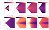 |
Fig. B.1 Density profile on the first row and temperature profile on the second, for the DiskFit best models. The 1st column is for dust, the 2nd for 13CO, the 3rd for 12CO (2-1) and (3-2) and the 4th for HCO+. The solid vertical line represents the beam, and the curved horizontal lines correspond to one and two scale heights. Note: the density profile scale (in cm−3) is expressed in log10. The densities shown for the molecular tracers correspond to the number density of the specific molecule, not the total H2 density, and are therefore several orders of magnitude lower than dust-derived gas densities. |
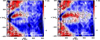 |
Fig. B.2 Differences TRD (observation TRD - model TRD) of the 12CO 2-1 emission after fitting a model with depletion (on the left) and without depletion (on the right). Color scale spans and contours are defined from −3 K to 3 K in steps of 1 K. |
All Tables
All Figures
|
Fig. 1 Continuum observations. Left column (a): observation. Middle column (b): best model. Right column (c): difference (observation - model). The rms noise levels reach 0.1 K at 146 GHz, 6.55 × 10⁻³ K at 225 GHz, and 1.33 × 10⁻² K at 333 GHz. The peaks of the residuals correspond to 5.2σ at 146 GHz, 11.8σ at 225 GHz, and 8.7σ at 3 33 GHz. |
| In the text | |
|
Fig. 2 Integrated-intensity map of 12CO 2-1 (left, clipped at 22 mJy/beam km/s), and integrated-intensity map of HCO+ 3-2 (right, clipped at 8 mJy/beam km/s). The maps are rotated by −73.5°. The contours are defined from 0 to 0.1 Jy/beam km/s in steps of 0.01 Jy/beam km/s, i.e., 3.36σ for the 12CO 2-1 map, and from 0 to 0.5 Jy/beam km/s in steps of 0.02 Jy/beam km/s , i.e., 2.30σ for the HCO+ 3-2 map. |
| In the text | |
|
Fig. 3 Montage of JWST and interferometric data for SSTTau042021. MIRI MRS images from JWST reveal H2 S(2) emission at 12.278-μm (Arulanantham et al. 2024). The white contours indicate the mid-infrared scattered-light continuum at 12.2-μm, and the dashed white line marks the rotation axis of the disk at PA = 73.5°. In archival ALMA data and new NOEMA observations, the cyan contours show molecular emission lines of HCO+ 3—2, 13CO 2—1, C18O 2-1, 12CO 2-1, and 12CO 3-2, and the yellow contours represent the 0.85 mm continuum emission at 1 mJy/beam. The beige circles in the bottom left corner of each panel represent the average theoretical FWHM of the PSF for JWST data, calculated from the relation reported by Law et al. (2023), and the beam of the molecular line emission is shown as a cyan ellipse in the top right corner of each panel. The contours for HCO+ (3-2) range from 0.02 to 0.2 Jy/beam km/s with a step of 0.02 Jy/beam km/s, i.e., 2.5 œ; for 13CO (2-1), they range from 0.02 to 0.08 Jy/beam km/s with a step of 0.01 Jy/beam km/s, i.e., 3.5 œ; for C18CO (2-1), they range from 0.008 to 0.016 Jy/beam km/s with a step of 0.008 Jy/beam km/s, i.e., 3.5 œ; for 12CO (2-1), from 0.01 to 0.08 Jy/beam km/s with a step of 0.02 Jy/beam km/s, i.e., 6 œ; and for 12CO (3-2), from 0.06 to 0.8 Jy/beam km/s with a step of 0.06 Jy/beam km/s, i.e., 4.2σ. |
| In the text | |
|
Fig. 4 From top to bottom: TRD of 12CO 2-1, 12CO 3-2, 13CO 2-1, C18O 2-1 and HCO+ 3-2: (a) TRD of the observations. (b) TRD of the final result of the models. (c) Difference between the observations and model TRD. For 12CO (2-1), the residuals range from −2 to 2 K, while for the 12CO (3-2) transition, they extend from −3 to 2 K. In the case of 13CO (2-1), the differences are between 0 and 2 K. For C18O (2-1), the deviations range from −1 to 2 K, and for HCO+ (3-2), they span from −1 to 3 K. The vertical black line represents the effective resolution, and the two error bars show the widening of the beam as a function of radius caused by the TRD method. The contours are defined from 4 K to 20 K in steps of 2 K for the observational and model maps, and from −3 K to 3 K in steps of 1 K for the residual maps. |
| In the text | |
|
Fig. 5 As in Figure 3, overlay of the JWST image from Arulanantham et al. (2024) with contours of the 12CO (2-1) channel maps at 6.80 km/s and 8.23 km/s illustrating the large vertical extent around the H2 emission. The contours are in steps of 3.4σ and range from 10 to 40 mJy beam−1. |
| In the text | |
|
Fig. A.1 Velocity channel maps from top to bottom: for 12CO 2-1, 3-2, 13CO 2-1, C18O 2-1 and HCO+ 3-2. The channels corrupted by the CO clouds along the line of sight are marked with a red cross. These channels were not used in the DiskFit analysis. All the maps are rotated by −73.5°. The contours are defined as follows: from 3 to 12 K in steps of 3 K (i.e., 3.6σ) for the 12CO 2-1, 3.3σ for 12CO 3-2, and 3.6σ for 13CO 2-1; from 2 to 6 K in steps of 2 K (i.e., 3.2σ) for C18O 2-1; and from 3 to 9 K in steps of 3 K (i.e., 3.3σ) for HCO+ 3-2. |
| In the text | |
|
Fig. B.1 Density profile on the first row and temperature profile on the second, for the DiskFit best models. The 1st column is for dust, the 2nd for 13CO, the 3rd for 12CO (2-1) and (3-2) and the 4th for HCO+. The solid vertical line represents the beam, and the curved horizontal lines correspond to one and two scale heights. Note: the density profile scale (in cm−3) is expressed in log10. The densities shown for the molecular tracers correspond to the number density of the specific molecule, not the total H2 density, and are therefore several orders of magnitude lower than dust-derived gas densities. |
| In the text | |
|
Fig. B.2 Differences TRD (observation TRD - model TRD) of the 12CO 2-1 emission after fitting a model with depletion (on the left) and without depletion (on the right). Color scale spans and contours are defined from −3 K to 3 K in steps of 1 K. |
| In the text | |
Current usage metrics show cumulative count of Article Views (full-text article views including HTML views, PDF and ePub downloads, according to the available data) and Abstracts Views on Vision4Press platform.
Data correspond to usage on the plateform after 2015. The current usage metrics is available 48-96 hours after online publication and is updated daily on week days.
Initial download of the metrics may take a while.