| Issue |
A&A
Volume 704, December 2025
|
|
|---|---|---|
| Article Number | A299 | |
| Number of page(s) | 13 | |
| Section | Astrophysical processes | |
| DOI | https://doi.org/10.1051/0004-6361/202554928 | |
| Published online | 17 December 2025 | |
A simple toy model for the electromagnetic variability of lump-dominated circumbinary disks around binary black holes
1
Department of Physics, Norwegian University of Science and Technology, NO-7491 Trondheim, Norway
2
Université Paris Cité, CNRS, Astroparticule et Cosmologie, F-75013 Paris, France
3
Department of Theoretical Physics, Atomic and Optics, Campus Miguel Delibes, University of Valladolid, Paseo Belén, 7, 47011 Valladolid, Spain
4
Aix-Marseille Université, CNRS, CNES, LAM, Marseille, France
5
Université Paris-Saclay, Université Paris Cité, CEA, CNRS, AIM, 91191 Gif-sur-Yvette, France
★ Corresponding author This email address is being protected from spambots. You need JavaScript enabled to view it.
Received:
1
April
2025
Accepted:
23
October
2025
Abstract
Context. The electromagnetic detection of circumbinary disks around pre-merger binary black holes (BBHs) relies on theoretical predictions. These are generally obtained through expensive numerical simulations, but simple or fast toy models are lacking to unleash the potential of these theoretical advances for observational purposes.
Aims. We present a simple toy model for computing the electromagnetic variability of circumbinary disks around circular-orbit BBHs at relativistic separations. We focus on the effect of disk nonaxisymmetries.
Methods. We assumed that the disk is threaded by spiral arms and hosts a hotspot linked to an overdense structure (the lump) that is preferably reported in binaries of a close to equal mass. We built a simple temperature distribution and estimated its thermal emission, perceived by a distant observer, via a ray-tracing code in a BBH approximate metric. We propose a toy model that reproduces the main light-curve features and show that it is consistent with 2D general relativistic hydrodynamical simulations under the assumption of compressional heating and expansional cooling, except for purely dynamical effects such as the binary-lump beat.
Results. The light curve exhibits a main modulation at the lump period (i.e., a few times the orbital period) due to the relativistic Doppler effect, and a shorter modulation at the orbit-like period due to spiral arms or the beat. These are more prominent in the optical/UV band for a total binary mass M = 104 − 10 M⊙, where the disk energy spectrum peaks. For M = 109 M⊙, a lump modulation with an amplitude of 4% is detectable with the Vera Rubin Observatory after six months of observations up to z = 0.5.
Conclusions. We proposed a new simple toy model that can be used, for instance, to test the compatibility of the periodicity of BBH candidate sources with a circumbinary disk origin.
Key words: accretion, accretion disks / black hole physics / radiative transfer / relativistic processes / methods: numerical / quasars: supermassive black holes
© The Authors 2025
 Open Access article, published by EDP Sciences, under the terms of the Creative Commons Attribution License (https://creativecommons.org/licenses/by/4.0), which permits unrestricted use, distribution, and reproduction in any medium, provided the original work is properly cited.
This article is published in open access under the Subscribe to Open model. This email address is being protected from spambots. You need JavaScript enabled to view it. to support open access publication.
1. Introduction
Supermassive binary black holes (SMBBHs) are thought to emit a copious amount of electromagnetic (EM) radiation prior to merger1, and their future EM observation is a milestone of the multimessenger era. Individual SMBHs reside at the centers of their host galaxies (e.g., Ferrarese & Ford 2005; Gültekin et al. 2009), and merging galaxies are therefore expected to provide a gas-rich environment for the SMBBH. Emitting lower-frequency gravitational waves (GWs) than the now widely detected stellar mass BBHs (Abbott et al. 2016, 2021, 2023), the most massive SMBBHs (total mass M > 108 M⊙) are now detectable with pulsar timing arrays (PTAs; e.g., Lommen 2015, Babak et al. 2016, Kelley et al. 2019) in the 1 nHz−1 μHz band, while BBHs with M = 104 − 7 M⊙ will be detectable with the Laser Interferometer Space Antena (LISA; Amaro-Seoane et al. 2017) in the 0.1 mHz − 1 Hz band. Interestingly, SMBBH GW detection with LISA might be possible days to months before the merger (see Mangiagli et al. 2020), which would leave room for pre-merger EM follow-up. The LISA error box can be as large as 10 − 1000 deg2, with numerous sources to search through to identify the origin of the GW signal. For this reason, numerous efforts have been undertaken to identify the clear EM signal of BBHs and to search for candidates (Liu et al. 2019; De Rosa et al. 2019; D’Orazio & Charisi 2023). The present paper is meant to support these efforts.
Studies dedicated to predicting such pre-merger EM signatures relied on analytical approaches and/or (magneto- )hydrodynamical simulations, deriving from a common agreement on the flow geometry when the mass ratio q of the binary is not too extreme (typically ∼0.1 − 1). For aligned circular binaries, it consists of the following: a cavity of about twice the orbital separation (Artymowicz & Lubow 1994) because no stable circular orbit exists there; two spiral waves threading the circumbinary disk (CBD; e.g., MacFadyen & Milosavljevié 2008), and spiral streams penetrating the cavity (Artymowicz & Lubow 1996) and eventually feeding individual accretion structures referred to as mini-disks around the BHs (e.g., Farris et al. 2014); finally, an overdensity called lump (Shi et al. 2012) that orbits at the inner edge of the CBD. In this context, our aim is to compute the EM observables that exclusively arise from the CBD around BBHs. This configuration is expected when gas is available (e.g., Artymowicz & Lubow 1996) at a separation compatible with LISA detection (Piro et al. 2022 and references therein). As we focus on the variability from the CBD, we purposely omit any other emission from possible mini-disks for now (e.g., Farris et al. 2015; D’Ascoli et al. 2018; Gutiérrez et al. 2022; Krauth et al. 2023; Franchini et al. 2024; Cocchiararo et al. 2024; Porter et al. 2025), whose contribution would add up to the CBD emission. In our model, we initially assumed a nonaxisymmetric temperature distribution in the CBD with perturbations from the lump and spiral arms.
The lump feature has been reported in a large set of CBD simulations around nearlycircular (eccentricity e ≲ 0.1; e.g., D’Orazio et al. 2024) binaries with mass ratios on the order of unity. This lump (Shi et al. 2012) term characterizes an asymmetry in the density (or m = 1 azimuthal mode, with m the mode number) located close to the inner CBD edge that orbits at ∼4 − 10 Porb (e.g., Shi et al. 2012, Mignon-Risse et al. 2023b), with Porb the binary period. Hence, this term does not refer to the underlying mechanism, but to a feature from CBDs that was unexpected, in particular, for initially symmetric (q = 1) systems. The interest in the lump comes from the intuitive prediction that it might eventually modulate the luminosity of CBDs as it orbits (see, e.g., Gold 2019) and/or modulates the accretion rate (e.g., Muñoz et al. 2020), but also that its associated gravitational torque might affect the orbital evolution of the central binary (Tiede et al. 2020). The lump has been reported in 2D (e.g., MacFadyen & Milosavljevié 2008; D’Orazio et al. 2013; Muñoz & Lai 2016; Miranda et al. 2017; Tang et al. 2017; Mösta et al. 2019; Muñoz et al. 2019; Tiede et al. 2020, 2022; Westernacher-Schneider et al. 2022; Siwek et al. 2022; Krauth et al. 2023; Wang et al. 2023b; Mahesh et al. 2024) and 3D simulations. They included grid-based (Moody et al. 2019; Shi & Krolik 2015) and smoothed-particle hydrodynamic (Ruge et al. 2015; Heath & Nixon 2020; Ragusa et al. 2020; Franchini et al. 2022, 2024) studies. In the angular momentum transport mechanism, the lump was found in nonviscous (e.g., Mignon-Risse et al. 2023b; Cimerman & Rafikov 2024), viscous (e.g., Farris et al. 2014, 2015), hydrodynamical, and magnetohydrodynamical (e.g., Shi et al. 2012) and radiation-magnetohydrodynamical (Tiwari et al. 2025) simulations. It was also present regardless of the gravity description: Newtonian (e.g., Dittmann & Ryan 2022), post-Newtonian (Liu 2021), or general relativistic (GR, e.g., Noble et al. 2012; Gold et al. 2014; Zilhão et al. 2015; Noble et al. 2021; Lopez Armengol et al. 2021; Mignon-Risse et al. 2023b). For circular binaries, it was found to form when q is not too far from unity (q ≳ 0.25, D’Orazio et al. 2013; q ≳ 0.1, Mignon-Risse et al. 2023b; q ≳ 0.5, Noble et al. 2021). Because the orbital separation can be and was used to renormalize distances in most Newtonian studies (e.g., Miranda et al. 2017), the lump might be a common feature at all orbital separations that allow for the presence of a CBD. Hence, these works suggested that the lump is a robust feature from CBDs orbiting circular binaries of comparable masses.
Moreover, CBDs exhibiting a lump are likely to possess a nonaxisymmetric temperature distribution with m = 1 symmetry, as found by Tang et al. 2018; Gutiérrez et al. 2022; Cocchiararo et al. 2024; Tiwari et al. 2025, for instance. Possible causes are the enhanced shocks there (Shi et al. 2012; Cocchiararo et al. 2024), compressional heating, viscous heating (in the general sense, related to angular momentum transport; Cimerman & Rafikov 2024; see also the radial mass flux in Shi et al. 2012), or the indirect impact of a strongly enhanced density on the disk thermodynamics. Wang et al. (2023a) found the temperature distribution to be axisymmetric only in their locally isothermal CBDs, whereas it was nonaxisymmetric for any other choice of the so-called β-cooling timescale. Quantitatively, the temperature perturbation would naturally depend on the CBD thermodynamics, which has been modeled in several ways (see the references above) and is not well constrained at this stage. Hence, we chose to compute the temperature perturbations via a useful parametric approach encapsulating these uncertainties. In complement, the lump was proposed to be possibly linked to the Rossby wave instability (Mignon-Risse et al. 2023b), a well-studied instability (e.g., Tagger & Varniere 2006; Lovelace & Romanova 2014) that is known to develop at the edge of accretion disks (Lovelace et al. 1999). Thus, we can use these theoretical (knowing the instability criterion) or empirical arguments to extrapolate not only the spiral-wave-related, but also the lump-related emission modulation properties, at least qualitatively: This is the purpose of the present paper.
It is expected that the spectral energy distribution (SED) of the CBD peaks in the UV (Roedig et al. 2014; Farris et al. 2015; D’Ascoli et al. 2018; Gutiérrez et al. 2022; Krauth et al. 2023; Franchini et al. 2024) to soft X-ray (Tang et al. 2018) for M = 106 M⊙. For observers that do not observe face-on, any aforementioned nonaxisymmetry orbiting in the disk would produce an EM modulation (e.g., Varniere & Blackman 2005) at its orbital period as a consequence of self-shadowing. This is further amplified by relativistic effects.
GR effects can be decisive for computing the EM variability. They modify the observational appearance of disks around compact objects in various aspects (e.g., relativistic Doppler, gravitational beaming, and time delay), even for unresolved sources (e.g., Vincent et al. 2013). In the context of BBHs, relativistic Doppler (see, e.g., D’Orazio et al. 2015 in addition to mini-disk models) and gravitational beaming were accounted for by Tang et al. (2018), in addition to pseudo-Newtonian simulations, and by D’Ascoli et al. (2018), Gutiérrez et al. (2022), Porter et al. (2025) with a BBH metric. Here, we consider these GR effects by using an approximate BBH metric. Since the inner CBD edge is at a few times the separation, we expect relativistic effects (which are more intense in the vicinity of BHs) to be amplified at smaller separation. We therefore focused on relativistic separations (≲100 GM/c2) here. At these separations, the binary is thought to have already circularized efficiently through GW emission to reach an eccentricity e ≲ 0.1 that is compatible with the lump presence (D’Orazio et al. 2024), as discussed in our Appendix A (see also Zrake et al. 2021). Accordingly, we considered BBH systems with circular orbits.
The remainder of this paper is structured as follows. In Sect. 2 we present the CBD model and ray-tracing approach. In Sect. 3 we compute and characterize the thermal light curve (LC) variability owing to the CBD spiral arms and lump. Then, we propose a simple toy model for the LCs (Sect. 4). We show that it compares well with an LC produced from post-processed 2D general hydrodynamical simulations (Sect. 5), but in some cases, the second modulation can be at the beat frequency between the binary and the lump. We discuss the use of this toy model and apply it to searches with the Vera Rubin Observatory (VRO) in Sect. 6. We present our main conclusions in Sect. 7.
In the following, we use the unit system G = c = 1, so that the gravitational radius, rg = GM/c2, which is the natural length unit, and the associated time unit tg = GM/c3, are simply equal to rg = tg = M. In this system, spatial lengths and times are given in units of M with the conversion factor 1 M⊙ = 1.477 km = 4.926 × 10⁻⁶ s.
2. Simple representation of the CBD characteristics
We explored some of the thermal emission characteristics of near-circular BBH CBDs. Instead of performing the full GR-ray-tracing on many numerical simulations of CBDs to cover the vast parameter space (in mass, mass ratio, separations, accretion rate, etc.), we decided to start with a simplified parametric model exhibiting the key CBD characteristics that are found in most of the simulations of near-circular BBHs in the literature. The model was used to compute the frequency- and time-dependent emission in GR. The aim was to identify potential key observables and their relation to the binary parameters.
2.1. Key CBD characteristics
As already presented in the introduction, the CBDs key structures consist first of a disk with an edge around twice the binary separation (Roedig et al. 2014; Farris et al. 2015; D’Ascoli et al. 2018; Gutiérrez et al. 2022; Krauth et al. 2023; Franchini et al. 2024). We assumed this to be symmetric for simplicity. Second, we considered the so-called m = 1 lump which consists of an overdensity that orbits near the edge of the CBD and is related to the local orbital period there. Finally, we also added the m = 2 (two-arm) spiral embedded in the CBD that is linked with the orbital period of the binary (Tang et al. 2018; D’Ascoli et al. 2018; Duffell et al. 2020; Westernacher-Schneider et al. 2022; Cimerman & Rafikov 2024; Franchini et al. 2024; Cocchiararo et al. 2024).
2.2. Model of the temperature distribution
In order to mimic the key characteristics of the CBD, we used a similar method as Varniere & Vincent (2016), with an axisymmetric equilibrium disk that is perturbed by the spiral and the lump. Based on this complete temperature profile, we computed the blackbody emission of the multicolor disk.
To represent the unperturbed axisymmetric thermal emission component of the CBD, we used the standard model first presented by Shakura & Sunyaev (1973), which consists of a geometrically thin optically thick disk truncated at an inner radius rin = 2 b with b the separation (as in Roedig et al. 2014), with a monotonic temperature profile
 (1)
(1)
where  is the Eddington accretion rate, and with a standard radiative efficiency η = 0.1.
To add a hotter spiral and lump to the axisymmetric disk, we used the perturbation function presented by Varniere & Vincent (2016), which was successfully used to produce synthetic observations of accretion disks around BHs of various masses (Varniere et al. 2016; Varniere & Vincent 2017; Varniere 2023). The temperature is given as a function of time and position as
![Mathematical equation: $$ \begin{aligned} T(t,r,\varphi ) = T_0(r) \left[ 1 + \gamma _{\rm s/l} \left(\frac{r_{\rm c}}{r}\right)^{1/4}\ e^{\left(-\frac{1}{2}\left(\frac{r-r_{\rm s/l}(t,r,\varphi )}{ \delta \, r_{\rm c}}\right)^2\right)}\right]^2 , \end{aligned} $$](/articles/aa/full_html/2025/12/aa54928-25/aa54928-25-eq3.gif) (2)
(2)
where the amplitude of the temperature perturbation due to the nonaxisymmetric pattern is controlled by γs for the spiral and by γl for the lump. The choice of γl = 0.3, the highest value we considered, increased the temperature to T/T0 ∼ 1.7. In comparison, the simulations of Tang et al. (2018) showed a contrast in the effective temperature between the lump and its surroundings of a factor of T/T0 ∼ 2 or more (see their Fig. 1, bottom panel; the differences are visible despite the logarithmic scale). The simulations of Noble et al. (2021) included no temperature maps, but showed surface density contrasts of ∼2 (see their Figs. 13, 14). For simplicity, we assumed only adiabatic and reversible heating so that P ∝ Σ5/3 and T = P/Σ (ideal gas). This translates into a temperature perturbation of T/T0 ∼ 1.6. This is roughly consistent with the highest value of γl considered here. With a similar reasoning based on the spiral density maps in the 2D hydrodynamical simulations of Cimerman & Rafikov (2024), we assumed γs such that T/T0 ≲ 1.1 (for γl = 0). The radial extent of the pattern is controlled by δ, which we fixed to 0.2 for the lump and the spiral. The corotation radius of the pattern is rc = 2 b, and the shape function, rs(t, φ) (rl(t, φ)), encodes the geometrical aspect of the spiral (lump).
For the spiral linked to the binary period, we set  , where the Keplerian approximation as used, for example, by Lopez Armengol et al. (2021), is sufficiently accurate at the separations considered here and for the purpose of our simple model (a more accurate description can be obtained via the post-Newtonian equation of motion; e.g., Mignon-Risse et al. 2023a). The shape function reads
 (3)
(3)
with an azimuthal extent set to δs, φ = 0.1, compatible with Cimerman & Rafikov (2024). In the general case, it should depend on the aspect ratio of the disk, with thinner colder disks producing sharper spiral waves. We only considered one value here, however, to focus on other parameters (e.g., the perturbation amplitude γs/l).
For the lump, which orbits at frequency  , the shape function is
 (4)
(4)
with radial and azimuthal extent parameters δl, r = 0.1 and δl, φ = 0.6, respectively2. With these assumptions, we fixed Ωl = Ωs/5, which sets rc slightly beyond rin, the edge of the CBD. These are approximations because the inner edge of the CBD is not exactly at twice the separation and because we negleted the cavity eccentricity (e.g., Duffell et al. 2024), although it is lower in GR than in Newtonian dynamics (Noble et al. 2012, 2021).
The effect of this nonaxisymmetrical structure on the temperature profile was previously shown to lead to quasi-periodic EM modulation in single BH disks (Varniere et al. 2019), in particular, because of the relativistic Doppler effect (Vincent et al. 2013).
2.3. Ray-tracing with gyoto
The temperature distribution presented above was then used as an input for the GR ray-tracing code gyoto3 (Vincent et al. 2011) in a time-dependent BBH spacetime that is valid down to b ∼ 8 M (the so-called near zone; Mundim et al. 2014; Ireland et al. 2016; Mignon-Risse et al. 2023a; and it also includes the far zone, which is valid beyond a gravitational wavelength from the binary, Johnson-McDaniel et al. 2009) to obtain multiwavelength thermal emission maps as shown in Fig. 1, and from there, the LCs. It might seem contradictory to couple our simplified disk model with a full ray-tracing method, but the importance of performing this ray-tracing was previously shown when variability in single BH disks was studied (Varniere & Vincent 2016; Casse & Varniere 2018).
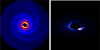 |
Fig. 1. Emission maps with the {disk + spiral} temperature distribution computed at inclination i = 20° (left panel; γs = 0.5) and the {disk + lump} temperature distribution computed at inclination i = 70° (right panel; γl = 0.3). The value of γs is higher than in the remainder of the paper. It was chosen to enhance visibility. |
One example is the relativistic Doppler effect, whose amplitude can be roughly estimated in an equivalent Schwarzschild metric (e.g., Tang et al. 2018). The intensity amplification is indeed proportional to 𝒟3 with 𝒟 = [Γ(1 − v∥)]−1, where v∥ is the gas velocity parallel to the observer’s line of sight, defined as v∥ = vcos(ϕ)sin(i), with v the gas velocity, ϕ the azimuthal angle with respect to the line of sight, and i the inclination angle. Considering an orbiting, warm lump as it approaches the observer, we simply used vϕ, the azimuthal velocity, as vcos(ϕ), and because it orbits close to the local Keplerian velocity, we obtained
![Mathematical equation: $$ \begin{aligned} \mathcal{D} ^3(r_{\rm l},i) \sim \left[ \frac{1 - (r_{\rm l}/M)^{-1} }{1 - (r_{\rm l}/M)^{-\frac{1}{2}} \mathrm{sin}(i) } \right]^3. \end{aligned} $$](/articles/aa/full_html/2025/12/aa54928-25/aa54928-25-eq8.gif) (5)
(5)
For rl = 2 b, b = 20 M, and i = 70°, this gives an intensity boost equal to 𝒟3 ∼ 1.5, which explains why these relativistic effects need to be incorporated.
The CBD was assumed to be optically thick and to be fully located in the z = 0 plane. The emission follows Planck’s law, and the intensity was computed as Iν = Bν(T(r, φ)), with Bν the Planck function. Null geodesics were backward-integrated from the observer to the emitting plasma, until they hit the disk plane. Hence, absorption and scattering were neglected here. When the geodesics intersected the plasma, its temperature and velocity at the time of emission were taken from the model. In this procedure, the time-dependence of the metric is accounted for because photons travel with a finite velocity (no fast-light approximation).
Unless stated otherwise, we computed spectra and LCs for a distance of D = 500 Mpc, a total binary mass of M = 4 × 10⁶ M⊙, and an accretion rate of Ṁ = 0.5 ṀEdd. At a fixed accretion rate in Eddington units, however, our temperature normalization assumed T ∝ M−1/4 (Eq. 1), so that the total flux integrated over a source with a surface of ∝rg2 ∝ M2 scales as F ∝ T4rg2 ∝ M (e.g., Roedig et al. 2014). Thus, as we focused on the shape of the LC modulation, we computed the frequency-integrated flux and renormalized it by the time-averaged flux. The resulting LCs are independent of mass when they are normalized.
3. An energy-dependent variability for the CBD
From previous work, we know that nonaxisymmetrical structures in the temperature profile of BH disks cause some almost periodic oscillations in the thermal radiative emissionof the disk (Varniere et al. 2019). We studied them in the context of CBDs in an approximate BBH spacetime (a Schwarzschild metric was instead used by Tang et al. 2018) that included gravitational redshift, a relativistic Doppler effect, and varying temperature perturbation parameters. We investigated their shape, energy dependence, and the effect of the intrinsic system parameters.
3.1. Energy dependence of the variability
One of the interesting observational aspects of an orbiting nonaxisymmetrical structure in the temperature distribution is the changing shape of its SED along the orbit of this structure (Varniere et al. 2020). We focused on the temporal evolution of the SED for our CBD model and therefore considered as a first example a separation b = 20 M and temperature perturbations with γl = 0.1 (T/T0 ∼ 20%) and γs = 0.02 (T/T0 ∼ 4%).
Figure 2 shows the energy spectrum at several instances in a portion of the lump orbit. At a frequency below 1015 Hz for our choice of mass M = 4 × 10⁶ M⊙, the SED shows no noticeable changes. At a higher frequency, however, the SED pivots toward a higher flux because it is linked to the innermost warmest parts of the CBD. This behavior is thus qualitatively independent of the perturbation parameters. The flux increases by a factor of ∼1.1 at 3 × 10¹⁵ Hz, where the (mean) SED peaks, and it increases by a factor of ∼2 at 1016 Hz. As a function of time, it will therefore create a strong modulation of the LC in the lump orbit. The amplitude of the flux modulation always depends on the frequency band at which it is computed.
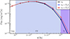 |
Fig. 2. Evolution of the SED along the lump orbit with Pl = 2π/Ωl for the model parameters γl = 0.1, γs = 0.02, b = 20 M for a mass M = 4 × 10⁶ M⊙ seen at an inclination angle of 70°. The initial time here, t0, was chosen to correspond to a minimum value of the flux. |
This case illustrates the frequency dependence of the expected flux modulation through the temporal evolution of the SED. We wish to present mass-independent LCs, however, and we therefore present below LCs that were computed by integrating the spectrum over all frequencies and that were normalized to the time-averaged bolometric flux (as mentioned in Sect. 2.3).
3.2. Effect of the binary parameters on the variability
One benefit of using a simple parametric model is that we can explore the effect of the binary or orbital parameters on the resulting flux modulation at a reasonable cost. Beyond the expectation of a modulation, nontrivial outcomes are the modulation shape and amplitude, in particular, in a BBH metric, and their dependence on the system parameters. Because the radius of the inner CBD edge and the binary period depend only slightly on the mass ratio (Noble et al. 2021), a more important binary-related parameter to be varied is the separation (see Sect. 2.2), especially in the context of mass-independent LCs.
From Fig. 2 we expect a modulation of the flux that is linked with the orbital period of the lump, which itself is linked to the binary period, and therefore, to its separation (Sect. 2.2). If this is similar to the single-BH case (Varniere & Vincent 2016), we would also expect a smaller modulation because the spiral orbits at half the binary period. This is confirmed by the LCs in Fig. 3. At two different orbital separations (b = 20 M and b = 30 M), this figure shows the normalized bolometric LC of the same parameters as for the temperature perturbations (γl = 0.3 and γs = 0.05, which are higher values than previously to enhance the visibility of the smaller-amplitude modulation).
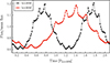 |
Fig. 3. Bolometric flux, normalized by the average between the minimum and maximum values, as a function of time for b = 20 M (black curve and stars) and b = 30 M (red curve and dots). The two LCs were computed for γl = 0.3, γs = 0.05, i = 70°, with 0° corresponding to a face-on view. |
In both cases, two modulations are visible on the LC. The dominant modulation is ∼20%, and the other modulation with the shorter period reaches a maximum of ∼5%. The shape of the dominant modulation is roughly sinusoidal. As expected, the dominant modulation is caused by the orbiting lump, and the smaller-amplitude modulation arises from the two-arm spiral that propagates in the disk at the binary period.
3.3. Amplitude of the temperature perturbation
One of the controversial aspects of the lump (a density feature by definition, Shi et al. 2012) that orbits at the edge of the CBD is by how much, if at all, it converts into an overheated lump in the temperature map as well (see for example Noble et al. 2012; Farris et al. 2015; Wang et al. 2023b, for different heating and cooling processes and their consequences on the lump). While there is some consensus about a modulation of the flux at near the period of the lump (e.g., Tang et al. 2018; Cocchiararo et al. 2024), the details of its origin are still debated. The different simulations of CBDs, with various heating and cooling processes, also rarely express quantitatively how the overdense lump structure translates into the temperature distribution. This hampers a study of the effect of the different heating efficiencies. By using our model, in which the heating efficiency is encapsulated in one parameter (i.e., the amplitude of the temperature perturbation), we explored the effect of a less efficient lump heating on the LC, and thus, on the detectability of the modulation.
In Fig. 4 we compare the amplitude of the main lump modulation when the associated temperature perturbation has γl = 0.3, versus the more conservative value γl = 0.1, for γs = 0.02. The lump remains the origin of the strongest modulation in both cases. More quantitatively, γl = 0.3 leads to a flux modulation with an amplitude of ±18%, and reducing it by a factor of three causes a flux modulation with an amplitude of ±4%. Although the spiral-related modulation is present by construction in the latter case, it is no longer visible by eye.
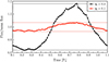 |
Fig. 4. Bolometric flux, normalized by the average between the minimum and maximum values, as a function of time for γl = 0.3 (black curve and stars) and γl = 0.1 (red curve and dots, corresponding to Fig. 2). The other parameters are fixed to i = 70°, γs = 0.02, and b = 20 M. |
This trend between the amplitude of the temperature perturbation and the amplitude of the flux modulation implies that even a temperature perturbation of a few percent might lead to a small but measurable modulation of the flux. An amplitude like this was indeed observed in the optical band, where the BBH candidate PG 1302-102 exhibits a modulation of 0.14 mag (Graham et al. 2015b), that is, ∼13% in our units. The lower the amplitude, the higher the number of periodic cycles covered by the data for a convincing detection (see, e.g., Cocchiararo et al. 2024).
4. Observational toy model for the CBD variability
After illustrating the relation of the LC and its modulations to the main intrinsic BBH parameters for a few cases, we focus on source-related parameters, such as the effect of the distance and inclination on the observables. We also studied the effect of the total binary mass on the modulation timescale and optimal frequency band. Based on all of this, we then present a simple toy model that will help in the search for CBD variabilities.
4.1. Effect of the distance and inclination
The observed radiative flux of a BBH system depends on the source distance D and inclination angle i. For the multicolor blackbody emission4 used here, both apply to the flux normalization, which is (rin/D)2 cos i.
All this is more complicated for the inclination because it is also related to GR effects. These GR effects tend to increase the amplitude of modulations from an orbiting nonaxisymmetric structure through Doppler boosting, and the effect increases with increasing inclination (from face-on to edge-on) and decreasing separation, as shown in Eq. (5). For completeness, we note that at the distance that separates the CBD from the BBH, the gravitational beaming is subdominant.
Fig. 5 shows this by comparing the amplitudes of the observed modulation from the same disk seen at two distinct inclinations, one more edge-on inclination at 70°, and another inclination that is closer to face-on at 20°. While the modulation is still present and detectable, the amplitude of the low-inclination LC is ±10%, and it is ±24% at a higher inclination. This means that modulations from systems that are seen close to face-on will be harder to detect.
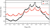 |
Fig. 5. Bolometric flux, normalized by the average between the minimum and maximum values, as a function of time for i = 70° (black curve and stars) and i = 20° (red curve and dots). The other parameters are fixed to γl = 0.3, γs = 0.05, and b = 20 M. |
4.2. Mass dependence and optimal observation band
In addition to the distance and inclination, another variable that is related to the source is its mass. We have so far shown renormalized LCs, that is, LCs without their mass dependence. As already suggested by the SED shown in Fig. 2, similar results are obtained when the LC is computed by integrating the flux over all frequencies or only in the frequency range around the emission peak.
In order to determine the optimal observation frequency band for the LC modulation, we need to estimate the frequency at which the SED of the CBD peaks as function of the binary mass and separation, denoted νmax. We obtained it by applying Wien’s law to the temperature of the inner CBD edge (see Eq. (1)). We show the color map of νmax as a function of M and the time to merger in Fig. 65. The time to merger was evaluated using the leading-order expression (Peters 1964) ; it gives the correct order-of-magnitude estimate, but becomes less accurate closer to merger. Most notably, Fig. 6 shows that the CBD peak frequency νmax is in the UV band for most SMBBH system parameters. This agrees with most simulations (e.g., Cocchiararo et al. 2024, Tiwari et al. 2025). For PTA sources (M ≥ 108 M⊙), νmax is in the optical band when the orbital separation is large enough, which corresponds to decades away from merger. This coincides with the band that hosts most variable sources that are attributed to BBH candidates (Graham et al. 2015a).
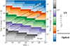 |
Fig. 6. Color map of the peak frequency in the emission spectrum of the CBD, νmax (in Hertz), as a function of the total binary mass M and the time to merger (in hours on the left, and in days on the right) derived from Eq. (1). This approximates the optimal energy band for observations of the LC modulations. The merger region is defined as b ≤ 1 M for simplicity. |
4.3. Toy model reproducing the main EM variability in the CBD
The results from the previous sections suggest that a simple analytical toy model can be created that reproduces the EM variability in the CBD model. We show below that the previous renormalized LCs can be fit by a simple sum of sinusoidal functionsin addition to the axisymmetric disk emission. This leads to the following model:
![Mathematical equation: $$ \begin{aligned} F(t)=F_0 \left[1 + A \cos \left( \frac{2 \pi t}{{P_{\rm l}}} + \phi \right) + A\prime \cos \left( \frac{2 \pi t}{{P\prime }} + \phi \prime \right) \right] , \end{aligned} $$](/articles/aa/full_html/2025/12/aa54928-25/aa54928-25-eq9.gif) (6)
(6)
with F0 the unperturbed disk flux (the peak emission is in the range shown in Fig. 6), and A and A′ are the respective amplitudes of the lump and spiral-related modulations, and ϕ, ϕ′ are their respective phases6. Pl is again the lump period, and P′ the orbit-related period, which results in Porb/2 for our symmetric spiral. For unequal-mass binaries, the spirals are likely to be asymmetric (e.g., Cimerman & Rafikov 2024) so that the dominant spiral would produce a modulation at P′ = Porb. We estimated the period of each modulation as
 (7)
(7)
with the lump period taken as an average between various numerical studies (e.g., Noble et al. 2012; Westernacher-Schneider et al. 2022).
The q-dependence of Porb was not included because this dependence only affects Porb at the percent level. Similarly, the dependence of the lump orbital period on q, which corresponds to the Keplerian period at the inner edge of the CBD and thus depends on the inner CBD radius, is smaller than its empirical uncertainty in numerical studies (Sect. 2.1).
We show how this toy model (Eq. (6)) would fit the previously obtained LC in the top panel of Fig. 7. While it is not a perfect fit, it recovers the overall behavior of the LC, and the residuals are ∼1%. This simplified model does not have the aim to give the exact LC of a CBD, but intends to produce a fast estimate of the potential variability and its optimal observation range.
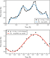 |
Fig. 7. Top panel: bolometric flux from our temperature model, normalized by the average between the minimum and maximum values, as a function of time (black curve and stars) and its fit by the toy model function (Eq. (6), blue curve). Bottom panel: rebinned normalized LC (stars) and its fit by the simplified toy model function (Eq. (9), red curve). The model parameters are fixed to γl = 0.3, γs = 0.05, b = 20 M, and i = 70°. |
This model can be simplified even further because the modulation linked to the binary is not only much faster than the modulation from the lump, but its amplitude is also far smaller. In practice, the spiral-related modulation might therefore not be detectable7. As a result, we omitted its contribution (the third term in Eq. (6)), especially when this period cannot be resolved by the available observations (see our discussion in Sect. 6). This gives the simplified version
![Mathematical equation: $$ \begin{aligned} F(t) = F_0 \left[1 + A \cos \left( \frac{2 \pi t}{\mathrm{P_{l}}} + \phi \right) \right] \quad \text{ if} \, \Delta t_{\rm obs} \gtrsim {P\prime }/5, \end{aligned} $$](/articles/aa/full_html/2025/12/aa54928-25/aa54928-25-eq11.gif) (8)
(8)
where we assumed at least five points per period to properly sample a given sinusoidal signal. This simpler version can always be used first, and by searching for any periodic structure in the residual, it can be decided whether the full version of the model is needed. The bottom panel of Fig. 7 shows the validation of the simplified toy model (Eq. (9)) against a rebinned LC. By rebinning, we mean that we defined coarser time bins Δtobs such that Δtobs > Porb/10, and we computed a flux average over each of these bins.
5. Comparison between the toy model and fluid simulations
As a test of how this simple toy model reproduces the main characteristics of more computationally expensive simulations, we present various fits of the LCs produced out of the q = 1, b = 20 M, and q = 0.1, b = 20 M runs presented by Mignon-Risse et al. (2023b) below, together with an additional simulation with q = 0.3, b = 36 M.
5.1. Outlook of the simulation setup and post-processing
These GR-AMRVAC (Casse et al. 2017) simulations consist of solving the conservation of the baryon density and momentum in the same BBH background metric as is used for the ray-tracing (Sect. 2.3). The thermodynamical gas behavior is isentropic, so that the total energy is conserved, and pressure evolves with the dynamics, unlike in the locally isothermal approximation. We used a polytropic equation of state with an adiabatic index γ = 5/3. The initial conditions corresponded to an axisymmetric disk with a warm (aspect ratio H/R ∼ 0.1) close to centrifugal equilibrium around an equivalent (M = M1 + M2) single BH. After an initial transient phase, in which the cavity developed self-consistently, spiral arms formed in the CBD, and the lump formed after some dozen BBH periods. They remained until the end of the simulation, that is, after 100 BBH periods (for more details, we refer to Mignon-Risse et al. 2023b).
The fluid temperature was computed as T ≡ P/Σ (with P the thermal pressure and Σ the surface density), which in our model meant that only compressional heating and expansional cooling were considered. This was used as input for the ray-tracing step. Without the fast-light approximation, one emission map calculation required several GR-AMRVAC outputs. Since the time of emission does not coincide in general with an output time, the variable was linearly interpolated among the GR-AMRVAC outputs.
5.2. EM variability
The top panel of Fig. 8 shows the bolometric LC normalized by the value averaged over the displayed time period (15 Porb), obtained from the post-processed fluid simulation with q = 1, b = 20 M, observed at an inclination of i = 70°. Two modulations are visible, and the dominant modulation lies at a period that is equal to the orbital lump period of ∼6 Porb. The orbital motion of the lump is illustrated by the fluid density map shown in the middle panel of Fig. 8 at the azimuthal angle φ = 3π/2. We obtained a nonaxisymmetric temperature distribution. This agrees with more sophisticated thermodynamical models, for instance, with Tang et al. (2018), who included viscous heating, shock heating, and radiative cooling. While this variability persists throughout the simulation (more than 60 Porb), each modulation period and amplitude depend on the instantaneous local condition in the disk (e.g., Varniere et al. 2020). A Fourier analysis of the LC, as shown in the bottom panel of Fig. 8, confirmed that the lump modulation strongly dominates in amplitude. The peak at the lump frequency has a high statistical significance because it is about 20 times the amplitude level at nearby frequencies. The zoom-in view shows weaker features at twice the binary-lump beat frequency (e.g., Roedig et al. 2011 in hydrodynamics, Noble et al. 2012; Shi et al. 2012; Combi et al. 2022; Tiwari et al. 2025 in magnetohydrodynamics) distributed over a range of frequencies near 1.5 Ωorb, and the spiral arms at frequency 2 Ωorb. Despite an amplitude of about six to ten times that of nearby frequencies, their firm detection is impeded by their weakness, the spread of the beat frequency, and the proximity of the two modes. The potential presence of the beat frequency is interesting because it is intrinsically related to the hydrodynamical problem. The amplitude of the orbital and beat modes might be amplified by the modulations from individual accretion structures, as reported by D’Orazio et al. (2015) and Bowen et al. (2018), respectively.
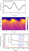 |
Fig. 8. Top panel: Normalized LC for q = 1, b = 20 M, seen at an inclination angle i = 70°. Two modulations dominate the LC, at the semi-orbital period and at the lump period. Middle panel: Density map in the (t, r)-plane for φ = 3π/2 (φ = 0 being the line of sight, it maximizes the Doppler effect) over the same period. Bottom panel: Amplitude of the Fourier modes in the LC, dominated by the lump modulation, and zoom-in view on the binary-lump beat signal, divided over a frequency interval, and the semi-orbital modulation. They are shown in power for clarity and are compared to a background red-noise fit of the form ω−α with α ∼ 2. |
5.3. Comparison and extension of the toy model
For this comparison, shown in Fig. 9, we considered three runs in which we varied the mass ratio or the orbital separation, all exhibiting the lump feature: q = 1, b = 20 M (top panel), q = 0.1, b = 20 M (middle panel), and q = 0.3, b = 36 M (bottom panel). We fit the LCs originating from the fluid simulations considering the main and longer-timescale modulation, using the simplified toy model, over one lump period to focus on the LC shape. The fit residuals are shown and expressed in %. The simplified toy model recovers the characteristic shape of the main LC, and the residuals mostly remain below 1%, but some points reach to 5%.
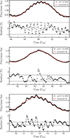 |
Fig. 9. LCs obtained from the fluid simulations, fit with a sinusoidal function (see Eq. 6), and fit residuals indicated in percent for q = 1, b = 20 M (top panel), q = 0.1, b = 20 M (middle panel), and q = 0.3, b = 36 M (bottom panel). The horizontal lines indicate the 1% level. All LCs were computed for an inclination of 70°. |
The residuals also show some sinusoidal substructures on shorter timescales than that of the lump for the q = 1, b = 20 M, and q = 0.3, b = 36 M cases. This might justify the use of the toy model with the shorter additional frequency, if the temporal resolution allows it. The secondary frequency is either compatible with the spiral arm frequency (q = 1, b = 20 M, top panel) or with the binary-lump beat (q = 0.3, b = 36 M, bottom panel). We expect that the relative importance of the modes depends on the disk thermodynamics and on various parameters: stronger spiral-arm modulations are hosted in more inclined and closer BBHs, while perfectly face-on systems are expected to only exhibit the beat modulation.
The simplified toy model reproduces the main characteristics of these simulated data from the CBD EM variability well overall. In addition to the lump, the imprint from a second modulation might be visible in the residuals depending on the system parameters and on the data quality. In this case, the toy model can be used with the second period, P′ in Eq. (6), corresponding either to the beat or to the spiral-related period.
6. Implications in the context of BBH detection
We present a few ways in which this simplified toy model can be used in the context of BBH detection or identification below. We discuss timescale constraints and estimate the detectability of the LC modulations in the optical band with the VRO.
6.1. Timescale limitations and the circular-orbit hypothesis
On their way to merger, accreting BBHs might go through two phases: (i) A slow inspiral, when the reference timescale (e.g., the lump period) can be considered constant over the exposure, cadence, and observation times, and (ii) a faster inspiral, during which this same period decay (in the pre-decoupling epoch; Tang et al. 2018; Dittmann et al. 2023) is no longer negligible over these observation-related timescales. Because we considered circular orbits for the BBH, this study implicitly describes (an asymptotical version of) the slow-inspiral phase. We present the consequences of the inspiral on the modulation periods below.
For reference, Fig. 10 illustrates the evolution of the three timescales of interest here, namely Porb/2 (or the beat period, which is on the same order), Pl, which are the two modulation timescales to sample, and the time to merger, for q = 1 as a function of M. As a guide, the time it takes for Pl to decrease by a factor X (such that the new period is X Pl with X < 1), denoted τcirc, X is given by the simple formula
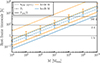 |
Fig. 10. Timescales of interest. Semi-orbital period (full line), lump period (dashed line), and time to merger, denoted τGW (dotted line), for the EM detection of a BBH CBD as a function of M for q = 1 and two values of b. |
 (9)
(9)
with τGW the initial time to merger (Peters 1964). In the pre-decoupling regime, this corresponds to a decrease in b of (1 − X2/3). This timescale is independent of the mass ratio. For illustration purposes, τcirc, 0.8 ∼ 0.45τGW; over this time, b decreases by 14%. If the integration time approaches τcirc, X with X such that the period decay is not negligible, the toy model and the analysis method should account for the decaying period. As an example, Fig. 10 shows that for M ≳ 108 M⊙, τcirc, 0.8 approaches typical optical LC timescales (hundreds of days to years; Graham et al. 2015a) for relativistic separations, in which case the inspiral might need to be taken into account.
Another aspect tangential to the toy model and its applications is the following. In order to detect a modulation, the instruments to which we have access must be able to sample it. On the other hand, the characteristic periods scale as M at fixed separation (in gravitational radii, which is the relevant unit for the dynamics), so that modulations in lower-mass systems occur on shorter timescales. For example, the Large Synoptic Survey Telescope8 (LSST), which surveys the entire sky every three days, will not be able to properly sample the lump period for systems with M ≪ 107 M⊙ at relativistic separations (Fig. 10).
6.2. Relevance of the circumbinary contribution to the variability of quasars
One of the interests of this model is that it can be used to test the viability of the BBH hypothesis for quasars that vary in the UV/optical band. We verified whether the modulation periods shown in Fig. 10 are already accessible with current detectors or even in archival data. As mentioned above, in the optical band, where the energy spectrum of the most massive (M ≥ 108 M⊙) system CBD peaks, ∼100 − 1000-day-long variability patterns have been reported in various studies dedicated to similarly high-mass BBH candidates (e.g., Graham et al. 2015b, Liu et al. 2019). In Fig. 10, these timescales fall into the range of the lump period for b = 50 M (M = 108 M⊙) or b = 20 M (M = 109 M⊙). We applied a similar reasoning in Foustoul et al. (2025) to derive the potential separation from the observed mass and periodicity. A similar or better sampling of the variability periods can be expected with recent and future EM facilities such as the LSST of the VRO.
As an example, we studied whether the LC modulations can be detected with the VRO and used the same method as Cocchiararo et al. (2024), assuming spiral arm and lump perturbations. We chose a set of parameters that was consistent with a CBD peak frequency in the G band ([5.43, 7.5]×1014 Hz) of b = 20 M and M = 109 M⊙, and we added Gaussian noise to the LC, with a variance equal to the 5σ sensitivity flux9, that is, 2.32 × 10⁻¹⁵ erg cm−2 s−1. Other radiation components were neglected. We considered a rather pessimistic case for the modulation amplitude, with γl = 0.1, γs = 0.02 (resulting in a ±4% dominant modulation; see Fig. 4). We considered three values for the distance10, D = 500 Mpc (z ∼ 0.1), D = 2.9 Gpc (z = 0.5), and D = 6.8 Gpc (z = 1), and performed Fourier transforms onto limited timescales of five and ten BBH orbits, with an orbital period of ∼34 d. For the parameters of this system, our circular-orbit model is still reasonable here because over one year of observations, the period decrease due to GW emission alone is minor (about 15% for q = 1, and less when q < 1; b decreases by 10%). The resulting Fourier amplitude normalized by the corresponding maximal amplitude is shown in Fig. 11. For a five-orbit integration, the lump modulation is visible up to z ∼ 0.511 ; for a ten-orbit integration (∼1 yr, one-tenth of the planned lifetime of VRO), its detection up to z = 0.5 is increasingly convincing with a ratio of 10 with respect to nearby frequencies; this is 100 when it is instead expressed in power (e.g., Noble et al. 2012). For z = 1, the noise dominates (the maximum is located beyond the displayed frequency range). Our results suggest that only a larger temperature perturbation would allow for a detection at z > 1. The spiral-related modulation is not detectable; a similar result would be obtained for the binary-lump beat with the same modulation amplitude. We specify that we used the synthetic LC here, but the toy model might instead be used to perform a similar exercise, but this time, to determine the minimum amplitude of the modulation that allows a detection at a given redshift.
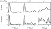 |
Fig. 11. Result of the Fourier transform onto synthetic LCs, in amplitude normalized by the maximum amplitude, for b = 20 M and M = 109 M⊙ for γl = 0.1 and γs = 0.02 for z ∈ {0.1, 0.5, 1}. The vertical dashed line indicates the orbital lump frequency. |
6.3. Estimating the LC modulation period for a GW event
A more direct use of this toy model is to help in the search for the EM counterpart of GW sources that are detected by LISA. While LISA will detect the GW signal from massive BBHs prior to the merger, the time that is available to find the source will range from months for the best cases to days and even hours before merger (Mangiagli et al. 2020). This means that we need a fast method that can provide the optimal energy band for a detection and the period (Eq. (8)) that is searched for. Our toy model will be able to provide these when the GW detection has given constraints on M, q, and on the time to merger, from which b is derived. This will allow us to focus our observations with the observatory that has the best chance to detect the variability.
Even more importantly, our toy model might also be used to investigate the history of the modulation and thus allow us to extend our search for the EM counterpart to a real-time search, but also using archival data of the region of interest (see Xin & Haiman 2024 on using LSST archival data to search for a LISA counterpart). This search could be automated because the binary separation can be extrapolated back in time, and our toy model can estimate the periodicity for any archival observation data of the region.
This approach can be taken a step further by considering the current characteristics of a potential future LISA source. This would allow us to compile a catalog of potential BBHs by the time LISA is launched, from which we could select the best target when LISA begins to detect GWs. This catalog would speed up the potential detection of the EM counterparts of the LISA detection.
7. Conclusions
We have constructed an analytical nonaxisymmetric CBD temperature distribution of BBH systems that incorporated commonly reported features of the CBD such as spiral arms and the lump. When they are ray-traced back to the observer in a BBH spacetime, these nonaxisymmetries produce sinus-like modulations in the UV/optical band for BBH masses M = 104 M⊙ to 1010 M⊙. We proposed a simple toy model that reproduces the LC variability from ray-traced LCs from this temperature distribution. It also reproduces the main characteristics of LCs from 2D GRHD simulations under the assumption of adiabatic heating/cooling, except for the binary-lump beat, which arises from the simulation and is intrinsically dynamical. The latter also produces a sinusoidal signal, however, and might be integrated to the toy model.
The advantage of this model lies in its simplicity. It might be used to fit optical/UV quasar LCs and retrieve the semi-orbital and/or lump period. Alternatively, in the LISA era, it might rapidly provide an estimate of the optimal energy band and variability timescale associated with the CBD thermal emission. This variability falls into the band of the VRO, the Hubble Space Telescope12, the Zwicky Transient Facility (ZTF)13, and the future UV Explorer14 and Habitable Worlds Observatory15. We showed that for b = 20 M and M = 109 M⊙, and in the absence of other contaminating radiation components, even a mild temperature perturbation from the lump would be detectable with the VRO up to z = 0.5 with six months to one year of observation. We recall, however, that detecting a variability is not a definitive test for BBHs because single BHs might also produce similar variabilities (Varniere et al. 2025).
We explicitly focused on the thermal CBD emission to take advantage of the progress made in the past years on the CBD dynamics and emission properties (see Gold 2019; D’Orazio & Charisi 2023 and references therein). Other sources of emission, including the thermal emission from the individual disks to begin with, would add to the CBD contribution, as well as their variability, albeit at higher frequency (e.g., Gutiérrez et al. 2022). In the case of quasars, obscuration by a dusty torus might drastically reduce the observed flux, especially at a high inclination, when the relativistic boost is strongest. These components will be included in future works.
While this work was developed, a tool for computing the EM variability of eccentric BBHs has been proposed by D’Orazio et al. (2024). They focused on accretion-rate related variability that affects the disk emission (to which a relativistic Doppler effect was applied), while we explicitly focused on a relativistic Doppler effect that directly acts on the nonaxisymmetric temperature distribution in the CBD to propose a toy model. Thus, we note the complementarity of the two approaches.
Data availability
The data that support the findings of this study are available from the corresponding author, R.M.R, upon request, and will also be part of a data release in 202516.
As the inspiral motion accelerates, the BBH might decouple from the circumbinary disk (Milosavljevic & Phinney 2005; Dittmann et al. 2023), affecting its EM appearance (Krauth et al. 2023; Franchini et al. 2024).
This gives a radial extent within the range reported in Noble et al. (2021) from the density distribution, and an azimuthal extent close to their lower-range value.
See the diskbb model at https://heasarc.gsfc.nasa.gov/xanadu/xspec/manual/node165.html
Here given for q = 1. To obtain the time to merger for other values of q, it should be multiplied by (1 + q)2/4q.
The amplitude of the modulation is related to the disk properties and to the distance to the source. It is therefore kept as a free parameter of the model. Similarly, the phase depends on the azimuthal position of each structure at the start of the observation.
The mini-disk variability due to Doppler boost, not included here, occurs on the same period as the spiral arms (e.g., D’Orazio et al. 2015). The toy model might be extended to include it, and the sum of both contributions might be detectable.
Starting from the LC at z ∼ 0.1 (Fig. 4), we rescaled the flux as a function of the distance as F ∝ D−2, but for simplicity, we did not apply the frequency redshift because this would require a fine-tuning of the mass or the separation to maintain the CBD peak frequency at the same value in the G band.
In comparison with the q = 1, e = 0 case of Cocchiararo et al. (2024), we obtain a better detectability of the lump. Indeed, although the normalized amplitude of the modulation is similar, by choosing a BBH mass of 109 M⊙ at relativistic separation instead of 106M⊙ at large (∼104rg) separation, our mean optical luminosity is ∼4 × 10⁻¹² erg cm−2 s−1 while theirs is ∼10−13 erg cm−2 s−1 at similar redshift (see their Fig. 6), enhancing the signal-to-noise ratio.
Which will be available for download at https://apc.u-paris.fr/~pvarni/eNOVAs/LCspec.html
Acknowledgments
RMR thanks A. Coleiro, P-A Duverne, F. Cangemi, V. Foustoul, A. Dittmann, D. D’Orazio and S. Lescaudron for useful discussions. RMR acknowledges funding from Centre National d’Etudes Spatiales (CNES) through a postdoctoral fellowship (2021-2023). RMR has received funding from the European Research Concil (ERC) under the European Union Horizon 2020 research and innovation programme (grant agreement number No. 101002352, PI: M. Linares). This work was supported by CNES, the LabEx UnivEarthS, ANR-10- LABX-0023 and ANR-18-IDEX-000, and by the Action Incitative: Ondes gravitationnelles et objets compacts and the Conseil Scientifique de l’Observatoire de Paris. This work was also supported by the Programme National des Hautes Energies (PNHE) of CNRS/INSU, co-funded by CNRS/IN2P3, CNRS/INP, CEA and CNES. The numerical simulations we have presented in this paper were produced on the platform DANTE (AstroParticule & Cosmologie, Paris, France) and on the high-performance computing resources from GENCI - CINES (grant A0100412463) and IDRIS (grants A0130412463 and A0150412463).
References
- Abbott, B., Abbott, R., Abbott, T. D., et al. 2016, Phys. Rev. Lett., 116, 061102 [CrossRef] [PubMed] [Google Scholar]
- Abbott, R., Abbott, B., Abbott, T. D., et al. 2021, Phys. Rev. X, 11, 021053 [Google Scholar]
- Abbott, R., Abbott, B., Abbott, T. D., et al. 2023, Phys. Rev. X, 13, 011048 [NASA ADS] [Google Scholar]
- Amaro-Seoane, P., Audley, H., Babak, S., et al. 2017, ArXiv e-prints [arXiv:1702.00786] [Google Scholar]
- Artymowicz, P., & Lubow, S. H. 1994, ApJ, 421, 651 [Google Scholar]
- Artymowicz, P., & Lubow, S. H. 1996, ApJ, 467, L77 [NASA ADS] [CrossRef] [Google Scholar]
- Babak, S., Petiteau, A., Sesana, A., et al. 2016, MNRAS, 455, 1665 [NASA ADS] [CrossRef] [Google Scholar]
- Bowen, D. B., Mewes, V., Campanelli, M., et al. 2018, ApJ, 853, L17 [NASA ADS] [CrossRef] [Google Scholar]
- Casse, F., & Varniere, P. 2018, MNRAS, 481, 2736 [NASA ADS] [CrossRef] [Google Scholar]
- Casse, F., Varniere, P., & Meliani, Z. 2017, MNRAS, 464, 3704 [Google Scholar]
- Cimerman, N. P., & Rafikov, R. R. 2024, MNRAS, 528, 2358 [NASA ADS] [CrossRef] [Google Scholar]
- Cocchiararo, F., Franchini, A., Lupi, A., & Sesana, A. 2024, A&A, 691, A250 [NASA ADS] [CrossRef] [EDP Sciences] [Google Scholar]
- Combi, L., Lopez Armengol, F. G., Campanelli, M., et al. 2022, ApJ, 928, 187 [NASA ADS] [CrossRef] [Google Scholar]
- D’Orazio, D. J., & Charisi, M. 2023, Observational Signatures of Supermassive Black Hole Binaries [Google Scholar]
- D’Orazio, D. J., Haiman, Z., & MacFadyen, A. 2013, MNRAS, 436, 2997 [Google Scholar]
- D’Orazio, D. J., Haiman, Z., & Schiminovich, D. 2015, Nature, 525, 351 [Google Scholar]
- De Rosa, A., Vignali, C., Bogdanovic, T., et al. 2019, New Astron. Rev., 86, 101525 [Google Scholar]
- Dittmann, A. J., & Ryan, G. 2022, MNRAS, 513, 6158 [NASA ADS] [Google Scholar]
- Dittmann, A. J., Ryan, G., & Miller, M. C. 2023, ApJ, 949, L30 [NASA ADS] [CrossRef] [Google Scholar]
- Duffell, P. C., D’Orazio, D., Derdzinski, A., et al. 2020, ApJ, 901, 25 [NASA ADS] [CrossRef] [Google Scholar]
- Duffell, P. C., Dittmann, A. J., D’Orazio, D. J., et al. 2024, ApJ, 970, 156 [NASA ADS] [CrossRef] [Google Scholar]
- D’Ascoli, S., Noble, S. C., Bowen, D. B., et al. 2018, ApJ, 865, 140 [CrossRef] [Google Scholar]
- D’Orazio, D. J., & Duffell, P. C. 2021, ApJ, 914, L21 [CrossRef] [Google Scholar]
- D’Orazio, D. J., Duffell, P. C., & Tiede, C. 2024, ApJ, 977, 244 [Google Scholar]
- Farris, B. D., Duffell, P., MacFadyen, A. I., & Haiman, Z. 2014, ApJ, 783, 134 [NASA ADS] [CrossRef] [Google Scholar]
- Farris, B. D., Duffell, P., MacFadyen, A. I., & Haiman, Z. 2015, MNRAS, 446, L36 [NASA ADS] [CrossRef] [Google Scholar]
- Ferrarese, L., & Ford, H. 2005, Space Sci. Rev., 116, 523 [Google Scholar]
- Foustoul, V., Webb, N. A., Mignon-Risse, R., et al. 2025, A&A, 699, A55 [NASA ADS] [CrossRef] [EDP Sciences] [Google Scholar]
- Franchini, A., Lupi, A., & Sesana, A. 2022, ApJ, 929, L13 [NASA ADS] [CrossRef] [Google Scholar]
- Franchini, A., Bonetti, M., Lupi, A., & Sesana, A. 2024, A&A, 686, A288 [NASA ADS] [CrossRef] [EDP Sciences] [Google Scholar]
- Gold, R. 2019, Galaxies, 7, 63 [Google Scholar]
- Gold, R., Paschalidis, V., Etienne, Z. B., Shapiro, S. L., & Pfeiffer, H. P. 2014, Phys. Rev. D, 89, 064060 [NASA ADS] [CrossRef] [Google Scholar]
- Graham, M. J., Djorgovski, S. G., Stern, D., et al. 2015a, MNRAS, 453, 1562 [Google Scholar]
- Graham, M. J., Djorgovski, S. G., Stern, D., et al. 2015b, Nature, 518, 74 [Google Scholar]
- Gutiérrez, E. M., Combi, L., Noble, S. C., et al. 2022, ApJ, 928, 137 [CrossRef] [Google Scholar]
- Gültekin, K., Cackett, E. M., Miller, J. M., et al. 2009, ApJ, 706, 404 [CrossRef] [Google Scholar]
- Heath, R. M., & Nixon, C. J. 2020, A&A, 641, A64 [NASA ADS] [CrossRef] [EDP Sciences] [Google Scholar]
- Ireland, B., Mundim, B. C., Nakano, H., & Campanelli, M. 2016, Phys. Rev. D, 93 [Google Scholar]
- Johnson-McDaniel, N. K., Yunes, N., Tichy, W., & Owen, B. J. 2009, Phys. Rev. D, 80 [Google Scholar]
- Kelley, L. Z., Charisi, M., Burke-Spolaor, S., et al. 2019, Multi-Messenger Astrophysics with Pulsar Timing Arrays [Google Scholar]
- Krauth, L. M., Davelaar, J., Haiman, Z., et al. 2023, MNRAS, 526, 5441 [NASA ADS] [CrossRef] [Google Scholar]
- Liu, W. 2021, MNRAS, 504, 1473 [NASA ADS] [CrossRef] [Google Scholar]
- Liu, T., Gezari, S., Ayers, M., et al. 2019, ApJ, 884, 36 [Google Scholar]
- Lommen, A. N. 2015, Rep. Prog. Phys., 78, 124901 [Google Scholar]
- Lopez Armengol, F. G., Combi, L., Campanelli, M., et al. 2021, ApJ, 913, 16 [NASA ADS] [CrossRef] [Google Scholar]
- Lovelace, R. V. E., & Romanova, M. M. 2014, Fluid Dyn. Res., 46, 041401 [NASA ADS] [CrossRef] [Google Scholar]
- Lovelace, R. V. E., Li, H., Colgate, S. A., & Nelson, A. F. 1999, ApJ, 513, 805 [NASA ADS] [CrossRef] [Google Scholar]
- MacFadyen, A. I., & Milosavljevié, M. 2008, ApJ, 672, 83 [NASA ADS] [CrossRef] [Google Scholar]
- Mahesh, S., McWilliams, S. T., & Pirog, M. 2024, ApJ, 973, 18 [Google Scholar]
- Mangiagli, A., Klein, A., Bonetti, M., et al. 2020, Phys. Rev. D, 102, 084056 [NASA ADS] [CrossRef] [Google Scholar]
- Mignon-Risse, R., Varniere, P., & Casse, F. 2023a, MNRAS, 519, 2848 [Google Scholar]
- Mignon-Risse, R., Varniere, P., & Casse, F. 2023b, MNRAS, 520, 1285 [NASA ADS] [CrossRef] [Google Scholar]
- Milosavljevic, M., & Phinney, E. S. 2005, ApJ, 622, L93 [CrossRef] [Google Scholar]
- Miranda, R., Muñoz, D. J., & Lai, D. 2017, MNRAS, 466, 1170 [NASA ADS] [CrossRef] [Google Scholar]
- Moody, M. S. L., Shi, J.-M., & Stone, J. M. 2019, ApJ, 875, 66 [NASA ADS] [CrossRef] [Google Scholar]
- Mundim, B. C., Nakano, H., Yunes, N., et al. 2014, Phys. Rev. D, 89 [Google Scholar]
- Murray, A. R., & Duffell, P. C. 2025, ApJ, 982, 113 [Google Scholar]
- Muñoz, D. J., & Lai, D. 2016, ApJ, 827, 43 [Google Scholar]
- Muñoz, D. J., Miranda, R., & Lai, D. 2019, ApJ, 871, 84 [CrossRef] [Google Scholar]
- Muñoz, D. J., Lai, D., Kratter, K., & Miranda, R. 2020, ApJ, 889, 114 [Google Scholar]
- Mösta, P., Taam, R. E., & Duffell, P. C. 2019, ApJ, 875, L21 [CrossRef] [Google Scholar]
- Noble, S. C., Mundim, B. C., Nakano, H., et al. 2012, ApJ, 755, 51 [NASA ADS] [CrossRef] [Google Scholar]
- Noble, S. C., Krolik, J. H., Campanelli, M., et al. 2021, ApJ, 922, 175 [NASA ADS] [CrossRef] [Google Scholar]
- Peters, P. C. 1964, Phys. Rev., 136, B1224 [NASA ADS] [CrossRef] [Google Scholar]
- Piro, L., Ahlers, M., Coleiro, A., et al. 2022, Exp. Astron. [Google Scholar]
- Porter, K., Noble, S. C., Gutiérrez, E. M., et al. 2025, ApJ, 979, 155 [Google Scholar]
- Ragusa, E., Alexander, R., Calcino, J., Hirsh, K., & Price, D. J. 2020, MNRAS, 499, 3362 [NASA ADS] [CrossRef] [Google Scholar]
- Roedig, C., Dotti, M., Sesana, A., Cuadra, J., & Colpi, M. 2011, MNRAS, 415, 3033 [NASA ADS] [CrossRef] [Google Scholar]
- Roedig, C., Krolik, J. H., & Miller, M. C. 2014, ApJ, 785, 115 [NASA ADS] [CrossRef] [Google Scholar]
- Ruge, J. P., Wolf, S., Demidova, T., & Grinin, V. 2015, A&A, 579, A110 [NASA ADS] [CrossRef] [EDP Sciences] [Google Scholar]
- Shakura, N., & Sunyaev, R. 1973, A&A, 24, 337 [Google Scholar]
- Shi, J.-M., & Krolik, J. H. 2015, ApJ, 807, 131 [NASA ADS] [CrossRef] [Google Scholar]
- Shi, J.-M., Krolik, J. H., Lubow, S. H., & Hawley, J. F. 2012, ApJ, 749, 118 [Google Scholar]
- Siwek, M., Weinberger, R., Muñoz, D. J., & Hernquist, L. 2022, MNRAS, 518, 5059 [NASA ADS] [CrossRef] [Google Scholar]
- Siwek, M., Weinberger, R., & Hernquist, L. 2023, MNRAS, 522, 2707 [NASA ADS] [CrossRef] [Google Scholar]
- Tagger, M., & Varniere, P. 2006, ApJ, 652, 1457 [NASA ADS] [CrossRef] [Google Scholar]
- Tang, Y., MacFadyen, A., & Haiman, Z. 2017, MNRAS, 469, 4258 [Google Scholar]
- Tang, Y., Haiman, Z., & MacFadyen, A. 2018, MNRAS, 476, 2249 [NASA ADS] [CrossRef] [Google Scholar]
- Tiede, C., Zrake, J., MacFadyen, A., & Haiman, Z. 2020, ApJ, 900, 43 [NASA ADS] [CrossRef] [Google Scholar]
- Tiede, C., Zrake, J., MacFadyen, A., & Haiman, Z. 2022, ApJ, 932, 24 [NASA ADS] [CrossRef] [Google Scholar]
- Tiwari, V., Chan, C.-H., Bogdanovic, T., et al. 2025, ApJ, 986, 158 [Google Scholar]
- Varniere, P. 2023, Astron. Nachr., 344, e220131 [Google Scholar]
- Varniere, P., & Blackman, E. 2005, New Astro., 11, 43 [Google Scholar]
- Varniere, P., & Vincent, F. H. 2016, A&A, 591, A36 [NASA ADS] [CrossRef] [EDP Sciences] [Google Scholar]
- Varniere, P., & Vincent, F. H. 2017, ApJ, 834, 188 [Google Scholar]
- Varniere, P., Mignon-Risse, R., & Rodriguez, J. 2016, A&A, 586, L6 [NASA ADS] [CrossRef] [EDP Sciences] [Google Scholar]
- Varniere, P., Casse, F., & Vincent, F. H. 2019, A&A, 625, A116 [NASA ADS] [CrossRef] [EDP Sciences] [Google Scholar]
- Varniere, P., Vincent, F. H., & Casse, F. 2020, A&A, 638, A33 [NASA ADS] [CrossRef] [EDP Sciences] [Google Scholar]
- Varniere, P., Mignon-Risse, R., & Casse, F. 2025, MNRAS, 538, 1055 [Google Scholar]
- Vincent, F. H., Paumard, T., Gourgoulhon, E., & Perrin, G. 2011, Class. Quantum Grav., 28, 225011 [Google Scholar]
- Vincent, F. H., Meheut, H., Varniere, P., & Paumard, T. 2013, A&A, 551, A54 [NASA ADS] [CrossRef] [EDP Sciences] [Google Scholar]
- Wang, H.-Y., Bai, X.-N., Lai, D., & Lin, D. N. C. 2023a, MNRAS, 526, 3570 [NASA ADS] [CrossRef] [Google Scholar]
- Wang, H.-Y., Bai, X.-N., & Lai, D. 2023b, ApJ, 943, 175 [NASA ADS] [CrossRef] [Google Scholar]
- Westernacher-Schneider, J. R., Zrake, J., MacFadyen, A., & Haiman, Z. 2022, Phys. Rev. D, 106, 103010 [NASA ADS] [CrossRef] [Google Scholar]
- Xin, C., & Haiman, Z. 2024, MNRAS, 533, 3164 [Google Scholar]
- Zilhão, M., Noble, S. C., Campanelli, M., & Zlochower, Y. 2015, Phys. Rev. D, 91, 024034 [Google Scholar]
- Zrake, J., Tiede, C., MacFadyen, A., & Haiman, Z. 2021, ApJ, 909, L13 [NASA ADS] [CrossRef] [Google Scholar]
Appendix A: Residual eccentricity at small separation
Lump disappearance has been found for binaries with eccentricity e > 0.1 in 2D locally isothermal CBDs, for example, by Siwek et al. 2022 while it has been reported for e = 0.9 (and q = 1) in 3D self-gravitating CBDs by Cocchiararo et al. (2024). Thus, while the overall impact of the binary eccentricity onto the lump formation is not settled yet, these studies agree when the orbit is circular. Hence, we check whether supermassive BBHs at relativistic separations, on which we focus here, have a residual eccentricity compatible with the lump’s presence. For this, we first compute the semi-major axis as a function of the eccentricity, using the post-Newtonian Eq. 5.48 of Peters (1964). We consider an initial eccentricity compatible with the equilibrium value from binary-disk interaction, i.e. e0 = 0.5 (D’Orazio & Duffell 2021, Zrake et al. 2021, Siwek et al. 2023; see also the observational study of Murray & Duffell 2025 on binary stars), or even higher, i.e. e0 = 0.8. For this first application, we neglect any mechanism increasing the eccentricity. Figure A.1 shows that the eccentricity reduces from e0 = 0.5 (resp. e0 = 0.8) to e < 0.1 as the semi-major axis decreases from an arbitrary initial value b0 to 0.73 b0 (resp. 0.33 b0) only. This illustrates the efficiency of GW-driven eccentricity damping and that BBHs reaching relativistic separations would likely have e < 0.1, thus being compatible with the lump’s presence.
If we assume an eccentricity equilibrium obtained through binary-disk interaction, this same mechanism could be at work and counteract the GW-driven eccentricity damping. Thus, let us compare the timescales of eccentricity increase and GW-driven damping. For the former, Siwek et al. (2023) found a few Myr for a binary accreting at its Eddington rate with a radiative efficiency ϵ = 0.1. For the latter, we compute it as τGW, e ≡ e/(de/dt) using Eq. 5.42 of Peters (1964) and find
 (A.1)
(A.1)
which is orders-of-magnitude shorter than the eccentricity increase timescale found by Siwek et al. (2023), at relativistic separations, even for more massive (109 M⊙) BBHs like PTA sources. This result agrees with a low residual eccentricity found by Zrake et al. (2021) when supermassive BBHs enter the LISA band. We conclude that supermassive BBHs at relativistic separations likely have a low eccentricity e < 0.1, compatible with the lump.
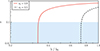 |
Fig. A.1. Eccentricity as a function of the orbital separation, for two initial eccentricities: e0 = 0.8 (red, full line) and e0 = 0.5 (black, dashed line). |
All Figures
|
Fig. 1. Emission maps with the {disk + spiral} temperature distribution computed at inclination i = 20° (left panel; γs = 0.5) and the {disk + lump} temperature distribution computed at inclination i = 70° (right panel; γl = 0.3). The value of γs is higher than in the remainder of the paper. It was chosen to enhance visibility. |
| In the text | |
|
Fig. 2. Evolution of the SED along the lump orbit with Pl = 2π/Ωl for the model parameters γl = 0.1, γs = 0.02, b = 20 M for a mass M = 4 × 10⁶ M⊙ seen at an inclination angle of 70°. The initial time here, t0, was chosen to correspond to a minimum value of the flux. |
| In the text | |
|
Fig. 3. Bolometric flux, normalized by the average between the minimum and maximum values, as a function of time for b = 20 M (black curve and stars) and b = 30 M (red curve and dots). The two LCs were computed for γl = 0.3, γs = 0.05, i = 70°, with 0° corresponding to a face-on view. |
| In the text | |
|
Fig. 4. Bolometric flux, normalized by the average between the minimum and maximum values, as a function of time for γl = 0.3 (black curve and stars) and γl = 0.1 (red curve and dots, corresponding to Fig. 2). The other parameters are fixed to i = 70°, γs = 0.02, and b = 20 M. |
| In the text | |
|
Fig. 5. Bolometric flux, normalized by the average between the minimum and maximum values, as a function of time for i = 70° (black curve and stars) and i = 20° (red curve and dots). The other parameters are fixed to γl = 0.3, γs = 0.05, and b = 20 M. |
| In the text | |
|
Fig. 6. Color map of the peak frequency in the emission spectrum of the CBD, νmax (in Hertz), as a function of the total binary mass M and the time to merger (in hours on the left, and in days on the right) derived from Eq. (1). This approximates the optimal energy band for observations of the LC modulations. The merger region is defined as b ≤ 1 M for simplicity. |
| In the text | |
|
Fig. 7. Top panel: bolometric flux from our temperature model, normalized by the average between the minimum and maximum values, as a function of time (black curve and stars) and its fit by the toy model function (Eq. (6), blue curve). Bottom panel: rebinned normalized LC (stars) and its fit by the simplified toy model function (Eq. (9), red curve). The model parameters are fixed to γl = 0.3, γs = 0.05, b = 20 M, and i = 70°. |
| In the text | |
|
Fig. 8. Top panel: Normalized LC for q = 1, b = 20 M, seen at an inclination angle i = 70°. Two modulations dominate the LC, at the semi-orbital period and at the lump period. Middle panel: Density map in the (t, r)-plane for φ = 3π/2 (φ = 0 being the line of sight, it maximizes the Doppler effect) over the same period. Bottom panel: Amplitude of the Fourier modes in the LC, dominated by the lump modulation, and zoom-in view on the binary-lump beat signal, divided over a frequency interval, and the semi-orbital modulation. They are shown in power for clarity and are compared to a background red-noise fit of the form ω−α with α ∼ 2. |
| In the text | |
|
Fig. 9. LCs obtained from the fluid simulations, fit with a sinusoidal function (see Eq. 6), and fit residuals indicated in percent for q = 1, b = 20 M (top panel), q = 0.1, b = 20 M (middle panel), and q = 0.3, b = 36 M (bottom panel). The horizontal lines indicate the 1% level. All LCs were computed for an inclination of 70°. |
| In the text | |
|
Fig. 10. Timescales of interest. Semi-orbital period (full line), lump period (dashed line), and time to merger, denoted τGW (dotted line), for the EM detection of a BBH CBD as a function of M for q = 1 and two values of b. |
| In the text | |
|
Fig. 11. Result of the Fourier transform onto synthetic LCs, in amplitude normalized by the maximum amplitude, for b = 20 M and M = 109 M⊙ for γl = 0.1 and γs = 0.02 for z ∈ {0.1, 0.5, 1}. The vertical dashed line indicates the orbital lump frequency. |
| In the text | |
|
Fig. A.1. Eccentricity as a function of the orbital separation, for two initial eccentricities: e0 = 0.8 (red, full line) and e0 = 0.5 (black, dashed line). |
| In the text | |
Current usage metrics show cumulative count of Article Views (full-text article views including HTML views, PDF and ePub downloads, according to the available data) and Abstracts Views on Vision4Press platform.
Data correspond to usage on the plateform after 2015. The current usage metrics is available 48-96 hours after online publication and is updated daily on week days.
Initial download of the metrics may take a while.