| Issue |
A&A
Volume 704, December 2025
|
|
|---|---|---|
| Article Number | A321 | |
| Number of page(s) | 21 | |
| Section | Numerical methods and codes | |
| DOI | https://doi.org/10.1051/0004-6361/202555307 | |
| Published online | 06 January 2026 | |
Rapid formation of a very massive star (>50000 M⊙), and subsequently, of an IMBH, from runaway collisions
Direct N-body and Monte Carlo simulations of dense star clusters
1
Astronomisches Rechen-Institut, Zentrum für Astronomie,
Mönchhofstrasse 12-14,
69120
Heidelberg,
Germany
2
Nicolaus Copernicus Astronomical Center, Polish Academy of Sciences,
Bartycka 18,
00-716
Warsaw,
Poland
3
Max-Planck-Institut für Astronomie,
Königstuhl 17,
69117
Heidelberg,
Germany
4
National Astronomical Observatories,
20A Datun Rd., Chaoyang District,
100101
Beijing,
China
5
Kavli Institute for Astronomy and Astrophysics, Peking University,
5 Yi He Yuan Road, Haidian District,
Beijing
100871,
China
6
Department of Physics, New York University Abu Dhabi,
PO Box 129188
Abu Dhabi,
UAE
7
Center for Astrophysics and Space Science (CASS), New York University Abu Dhabi,
PO Box 129188,
Abu Dhabi,
UAE
8
Dipartimento di Fisica, Sapienza Università di Roma,
Piazzale Aldo Moro 5,
00185
Rome,
Italy
9
Departamento de Astronomía, Facultad Ciencias Físicas y Matemáticas, Universidad de Concepción,
Av. Esteban Iturra s/n Barrio Universitario, Casilla 160-C,
Conc epción,
Chile
10
Gran Sasso Science Institute,
Viale F. Crispi 7,
67100
L’Aquila,
Italy
11
Physics and Astronomy Department Galileo Galilei, University of Padova,
Vicolo dell’Osservatorio 3,
35122,
Padova,
Italy
12
INFN – Laboratori Nazionali del Gran Sasso,
67100
L’Aquila, (AQ),
Italy
13
INAF – Osservatorio Astronomico d’Abruzzo,
Via M. Maggini snc,
64100
Teramo,
Italy
14
Faculty of Mathematics and Computer Science, A. Mickiewicz University,
Uniwersytetu Poznariskiego 4,
61-614
Poznari,
Poland
15
OzGrav: The ARC Centre of Excellence for Gravitational Wave Discovery,
Hawthorn,
VIC
3122,
Australia
16
Centre for Astrophysics and Supercomputing, Department of Physics and Astronomy,
John Street,
Hawthorn,
Victoria,
Australia
17
Main Astronomical Observatory, National Academy of Sciences of Ukraine,
27 Akademika Zabolotnoho St,
03143
Kyiv,
Ukraine
18
Departamento de Astronomía, Universidad de Chile,
Casilla 36-D,
Santiago,
Chile
19
Donostia International Physics Center,
Paseo Manuel de Lardizabal 4,
20118
Donostia-San Sebastián,
Spain
20
Universität Heidelberg,
Seminarstrasse 2,
69117
Heidelberg,
Germany
21
Department of Physics, Xi’an Jiaotong-Liverpool University,
111 Ren’ai Road, Dushu Lake Science and Education Innovation District,
Suzhou
215123,
Jiangsu Province,
PR China
22
Shanghai Key Laboratory for Astrophysics, Shanghai Normal University,
100 Guilin Road,
Shanghai
200234,
PR China
23
Department of Earth Science and Astronomy, College of Arts and Sciences, University of Tokyo,
3-8-1 Komaba,
Meguro-ku,
Tokyo,
153-8902,
Japan
24
Center for Information Science, Fukui Prefectural University,
4-1-1 Matsuoka Kenjojima,
Eiheiji-cho,
Fukui,
910-1195,
Japan
25
Center for Cosmology and Computational Astrophysics, Institute for Advanced Study in Physics, Zhejiang University,
Hangzhou
310027,
China
26
Institute of Astronomy, School of Physics, Zhejiang University,
Hangzhou
310027,
China
27
Max Planck Institute for Astrophysics,
Karl-Schwarzschild-Str. 1,
85741
Garching,
Germany
★ Corresponding authors: This email address is being protected from spambots. You need JavaScript enabled to view it.
; This email address is being protected from spambots. You need JavaScript enabled to view it.
Received:
26
April
2025
Accepted:
19
October
2025
Abstract
Context. We present simulations of a massive young star cluster using the codes Nbody6++GPU and MOCCA. The cluster is initially more compact than previously published models. It contains one million stars and has a total mass of 5.86 × 10⁵ M⊙ and a half-mass radius of 0.1 pc.
Aims. We analyzed the formation and growth of a very massive star (VMS) through successive stellar collisions and investigated the subsequent formation of an intermediate-mass black hole (IMBH) in the core of a dense star cluster.
Methods. We used direct N-body and Monte Carlo simulations that incorporated updated stellar evolution prescriptions for single and binary stellar evolution (SSE and BSE) tailored to massive stars and VMSs. These include revised treatments of stellar radii, rejuvenation, and mass loss during collisions. While the prescriptions represent reasonable extrapolations into the VMS regime, the internal structure and thermal state of VMSs that formed through stellar collisions remain uncertain, and future work may require further refinement. Results. Runaway stellar collisions in the cluster core produce a VMS that exceeds 5 × 10⁴ M⊙ within 5 Myr that subsequently collapses into an IMBH. We stress that further work on stellar astrophysics is needed, particularly in the context of VMS formation. The VMS formation currently represents strong uncertainties.
Conclusions. Our model suggests that dense stellar environments may enable the formation of VMSs and massive black hole seeds through runaway stellar collisions. These results provide a potential pathway for early black hole growth in star clusters and offer a theoretical context for interpreting recent observations with the James Webb Space Telescope of young compact clusters at high redshift.
Key words: methods: numerical / stars: black holes / stars: kinematics and dynamics / stars: massive
© The Authors 2026
 Open Access article, published by EDP Sciences, under the terms of the Creative Commons Attribution License (https://creativecommons.org/licenses/by/4.0), which permits unrestricted use, distribution, and reproduction in any medium, provided the original work is properly cited.
This article is published in open access under the Subscribe to Open model. This email address is being protected from spambots. You need JavaScript enabled to view it. to support open access publication.
1 Introduction
Most galaxies contain central supermassive black holes (SMBHs; 106−109 M⊙) that are embedded in a dense nuclear star cluster. Recent observations revealed even more massive SMBHs (1091010 M⊙) during the first billion years after the Big Bang (see Inayoshi et al. 2020 and, e.g., Adamo et al. 2024; Harikane et al. 2023; Kokorev et al. 2023, 2024; Goulding et al. 2023; Übler et al. 2023, 2024; Furtak et al. 2024; Matthee et al. 2024; Maiolino et al. 2024; Juodžbalis et al. 2024; Napolitano et al. 2025; Akins et al. 2025). This has sparked renewed interest in the question of the growth of these SMBHs in such a relatively short time if they grow via gas or star accretion from lower-mass seed black holes (BHs). Seed BHs are often identified with intermediatemass black holes (IMBHs; mass range of 102−105 M⊙; see for a review Greene et al. 2020), but seed BHs may have to be as massive as 106 M⊙ to explain the most massive SMBH in case of (super-)Eddington accretion (Shapiro 2005; Schneider et al. 2023).
The formation of central massive BHs from a primordial gas cloud in galactic nuclei was postulated by Rees (1984). The formation channels quoted in his famous Fig. 1 are a dense star cluster undergoing stellar collisions and mergers, a dense cluster of BHs, or a single supermassive star. We summarize the current ideas about these channels here following Inayoshi et al. (2020) and Volonteri et al. (2021).
Gravitational mergers between massive stars as a source of IMBH seeds have been discussed for decades (Sanders 1970; Lee 1987; Quinlan & Shapiro 1990; Portegies Zwart et al. 1999, 2004; Vanbeveren et al. 2009; Giersz et al. 2015; Mapelli 2016; Reinoso et al. 2020; Wang et al. 2022a; Rantala et al. 2024; Fujii et al. 2024b). This fast channel (a few million years after cluster formation and natal gas expulsion), following Greene et al. (2020), lead to the formation of a VMS by mass segregation and subsequent inelastic collisions of stars in the central region of a dense star cluster. We follow the definition of Fricke (1973); Hara (1978); Langbein et al. (1990) that a supermassive star (SMS) is characterized by the nonexistence of stable nuclear burning because the Kelvin-Helmholtz contraction directly leads to relativistic collapse. In the first cited paper by Fricke (1973), 5 ∙ 105 M⊙ was given as the limit, but the exact number depends on many parameters. Our massive object clearly stays below that limit and is therefore denoted as a VMS. One object outgrows the others by growing faster through collisions than its stellar evolution lifetime. This is often called runaway growth. This condition is not necessary for the collisional fast growth of a massive star. Most works so far either used a relatively small particle number for N-body simulations or approximate Fokker-Planck or Monte Carlo models. Until recently, computational limitations made N-body simulations with large particle numbers (>106) unfeasible. The analysis of observational data of nuclear star clusters (NSCs) and the comparison with relevant timescales further suggested that the collision time in these systems plays a critical role for the formation of their SMBHs (Escala 2021). In order to compare the collision timescale with the age of the system, Vergara et al. (2023) derived a critical mass scale for the formation of massive objects. This result was later extended to diverse stellar systems that encompassed various initial conditions, initial mass functions, and evolution scenarios (Vergara et al. 2024). Within the concept of critical mass, Liempi et al. (2025) successfully replicated the observed shape of the mass function between NSCs and SMBHs with semianalytic models.
Gravitational and general relativistic mergers between stellar mass BHs can lead to the formation of single massive BHs Zel’dovich & Podurets (1966). This idea was followed up by Rees (1984). This scenario was reevaluated in recent years and was rediscovered under the term of slow IMBH growth (about 100 Myr to billions of years). Mass segregation and stellar evolution generates central BH subsystems, but different from the ideas of (Zel’dovich & Podurets 1966), they are mixed with other stars and contain binaries. There are no purely single BH systems. These models have been shown to generate IMBHs with masses of about 102M⊙ to 104M⊙ (e.g., Portegies Zwart & McMillan 2002; Miller & Hamilton 2002; Giersz et al. 2015; Rodriguez et al. 2019; Arca Sedda et al. 2019, 2021a, 2023a; Di Carlo et al. 2020b,a; Kremer et al. 2020; Di Carlo et al. 2021 ; González et al. 2021 ; Leveque et al. 2022a; Maliszewski et al. 2022; Askar et al. 2023; Davis et al. 2024; González Prieto et al. 2024). The evolution toward an IMBH therefore depends sensitively on initial parameters such as the central density and the binary fraction (e.g., Rizzuto et al. 2021, 2022; Arca Sedda et al. 2021a; Arca-Sedda et al. 2021 ; Mapelli et al. 2022), and no phase of relativistic collapse of a BH subsystem is required (Zel’dovich & Podurets 1966). The presence of gas inflows, for example, after galaxy mergers, can substantially contribute to steepening the gravitational potential and enhancing the probability for collisions (Davies et al. 2011). As a result, this channel might contribute substantially to an explanation of the SMBH population (Lupi et al. 2014; Kroupa et al. 2020; Gaete et al. 2024).
The direct collapse of extremely massive gas clouds can result in massive BHs of about 104−106 M⊙ and effectively bypass all stellar evolution phases (e.g., Bromm & Loeb 2003; Begelman et al. 2006, 2008; Begelman 2010; Latif et al. 2013; Mayer et al. 2015). This channel is difficult to establish, however, because even trace amounts of dust, metals, or formation of molecular hydrogen might cause fragmentation (e.g., Omukai et al. 2008; Latif et al. 2014, 2016). The resulting objects are expected to form either supermassive stars or quasi-stars (BHs embedded in gaseous envelopes) that ultimately collapse to form massive BHs (Begelman et al. 2008; Hosokawa et al. 2013; Schleicher et al. 2013; Haemmerlé 2020; Kiyuna et al. 2024). We also include the possibility that stars might form with a high mass (105−106 M⊙) and might then explode as general relativistic instability supernovae (SNe; e.g., Shibata & Shapiro 2002; Sakurai et al. 2015; Uchida et al. 2017; Ugolini et al. 2025). Under more realistic direct collapse conditions, no simple direct collapse might be expected, but the possibility of fragmentation and subsequent mergers of the clumps has to be considered (e.g., Boekholt et al. 2018; Tagawa et al. 2020; Schleicher et al. 2022; Reinoso et al. 2023; Rantala et al. 2024; Kritos et al. 2024). The presence of strong far-ultraviolet radiation can allow the formation of stars that are more massive than 104 M⊙ at Z ≲ 10−3 Z⊙, while for Z≃ 10−2 Z⊙, fragmentation occurs that forms dense star clusters that can host stars with 103 M⊙ (Chon & Omukai 2025).
Massive Population III (Pop-III) stars have been postulated to produce seed IMBHs with masses of about 102 M⊙ through direct collapse above the pair-instability mass gap (e.g., Bromm & Larson 2004; Bromm 2013; Woosley 2017; Haemmerlé 2020; Mestichelli et al. 2024). (Extremely massive) Pop-III stars can merge with other Pop-III stars in their host clusters before collapse to produce even more massive IMBHs above the pair-instability mass gap during the fast gravitational runaway merger phase, as outlined above (e.g., Katz et al. 2015; Sakurai et al. 2017; Reinoso et al. 2018, 2020; Tanikawa et al. 2022; Wang et al. 2022a; Mestichelli et al. 2024). Collisions between Pop-III stars, which also accrete material at rates of 10−3 M⊙ yr−1, can lead to the formation of BHs with masses of about 104 M⊙ (Reinoso et al. 2025).
Previous work showed that rapid accretion can lead to very large radii of the supermassive stars that form in these scenarios (up to 100 AU for 104 M⊙ stars), particularly when the timescale for mass gain is shorter than the Kelvin-Helmholtz timescale of the stars (Hosokawa et al. 2013; Schleicher et al. 2013; Haemmerlé et al. 2018; Nakauchi et al. 2020). The formation of a VMS has been investigated by Nakauchi et al. (2020) with the modules for experiments in stellar astrophysics (MESA) (Paxton et al. 2011, 2013, 2015, 2018, 2019) to simulate the evolution of massive stars up to 3000 M⊙. It accounts for stellar wind mass loss from metal-poor to solar metallicity stars. The authors found that these stars grow from about 30 R⊙ at the MS to about 104 R⊙ in the post-MS phase. Martinet et al. (2023) also used the geneva stellar evolution code (GENEC) (Eggenberger et al. 2008) to model rotating and nonrotating stars of 180 to 300 M⊙ with a metallicity of Z = 0.014. They reported MS lifetimes of about 2.2-2.6 Myr.
Globular cluster formation takes place in the local Universe as well as at high redshifts (Adamo et al. 2024; Mowla et al. 2024, see discussion below). High-metallicity clusters may form from high-density gas clouds, for example, in merging galaxies or fragmented tidal arms, and they are frequently observed in interacting galaxies. The formation of low-metallicity clusters in the early universe in a cosmological context is quite difficult regarding the baryonic content of clusters. The metallicity range is very narrow and excludes a strong self-enrichment during the formation phase. Recently, Kimm et al. (2016) succeeded for the first time in simulating metal-poor globular clusters at high redshift (z > 7) during the epoch of reionization in dwarf galaxies in cosmological simulations. These metal-poor clusters were later accreted into Milky Way-type galaxies. Kimm et al. (2016) reported that two out of two simulated dwarf galaxies formed a globular cluster, which is more than sufficient to explain the observed population in the Milky Way. Still denser and/or more massive globular clusters might even be formed through this channel, considering that the authors modeled two randomly chosen halos.
Adamo et al. (2024) found that a few compact clusters with intrinsic masses of about 106 M⊙ formed 460 Myr after the Big Bang with the James Webb Space Telescope (JWST). The presence of extremely dense and massive clusters at high redshifts might be essential to explain the high nitrogen-oxygen abundances observed in galaxies (Bouwens et al. 2010; Tacchella et al. 2023; Marques-Chaves et al. 2024; Nagele & Umeda 2023). The VMSs that formed in these dense clusters might contribute to these observations through hydrogen-burning nucleosynthesis (Charbonnel et al. 2023). When the VMS is metal-enriched, it can emit powerful winds (Sander & Vink 2020; Vink 2022) that can enrich the gas with nitrogen at the expense of oxygen (Glebbeek et al. 2009). Supercompact massive star clusters can form during galaxy mergers (Renaud et al. 2015) that trigger starburst environments and create clusters with tens of thousands to millions of stars. High-redshift low-metallicity galaxies (Pettini et al. 1997) undergoing mergers are ideal environments for forming massive compact star clusters in which VMS can develop. In conclusion, we are motivated from theory, simulations, and observations alike to study the creation of VMSs in dense and massive star clusters that have formed in the early universe. We note that in the local Universe, the masses of the most massive detected stars are approximately 100-300 M⊙ (Doran et al. 2013; Keszthelyi et al. 2025). Beyond the local Universe, stars are too faint to measure their masses directly with current technology.
We provide N-body models for clusters that are very similar to the recently observed young massive clusters in the early universe (Mowla et al. 2024; Adamo et al. 2024), and we show how they would form a VMS and an IMBH. Our a full and direct star cluster N-body simulation also supports the longstanding conjecture that VMSs with masses of more than 104M⊙ form quickly and early therein by fast (possibly runaway) merging of normal stars with a massive star, as predicted by Monte Carlo simulations (see Sect. 2.2). Our N-body simulations used the code Nbody6++GPU, which is one of or maybe the most advanced and accurate integration code with regard to legacy, astrophysics, numerical and physical accuracy, and performance (Aarseth 1999a; Kamlah et al. 2022a; Spurzem & Kamlah 2023). This code is able to routinely simulate a globular-cluster size star cluster with all necessary astrophysical ingredients (Wang et al. 2015, 2016; Kamlah et al. 2022a; Arca Sedda et al. 2023a). While we used our code to simulate an unprecedentedly dense and massive star cluster, the huge computational costs limited the number of realizations to one. The formation and growth of an IMBH by mergers with other BHs will be a source of gravitational wave emission (Rizzuto et al. 2021; Arca Sedda et al. 2021b; Rizzuto et al. 2022) and tidal disruption events (Stone & Metzger 2016; Rizzuto et al. 2023).
The paper is organized as follows. Our method is summarized in Sect. 2. The initial conditions for the star clusters are presented in Sect. 3. We analyze our results in Sect. 4. A summary and conclusions are then presented in Sect. 5.
2 Methods
In this section, we present the method we employed, in particular, the code Nbody6++GPU in Sect. 2.1, and the code MOCCA is explained in Sect. 2.2. We explain in detail the new algorithms developed for the treatment of massive stars and VMS in Appendices A, B, C, D, E.
2.1 NBODY6++GPU
The dense star cluster models are evolved using the state-of-the-art direct force integration code Nbody6++GPU, which is optimized for parallelization using simultaneously three different levels, bottom-end of many core GPU accelerated parallel computing (Nitadori & Aarseth 2012; Wang et al. 2015), midlevel OpenMP thread based parallelization, and upper level MPI parallelization (Spurzem 1999). It yields excellent sustained performance on current hybrid massively parallel supercomputers (see Spurzem & Kamlah 2023, and Appendix F). It is a successor to the many direct force integration N -body codes of gravitational N-body problems, which were originally written by Sverre Aarseth (Aarseth 1985, 1999a,b, 2003b; Aarseth et al. 2008, and sources therein). The recent review by Spurzem & Kamlah (2023) provides a comprehensive overview over the entire research field of collisional dynamics and how Nbody6++GPU fits within this field. That review also provides some key informations about codes, such as PeTaR (Wang et al. 2020a) and BiFROST (Rantala et al. 2023).
The full scale parallel code still retains previously implemented features that are essential for efficient and accurate N -body integration on all scales. This includes the Hermite scheme with hierarchical block time-steps (McMillan 1986; Hut et al. 1995; Makino 1991; Makino & Aarseth 1992). The Ahmad-Cohen (AC) neighbour scheme (Ahmad & Cohen 1973) permits for every star to divide the gravitational forces acting on it into the regular component, originating from distant stars, and an irregular part, originating from nearby stars (“neighbours”). While the AC scheme is very efficient to reduce the number of floating operations necessary, it somewhat disturbs parallelization and acceleration, the code requires CPU and GPU (Wang et al. 2015). The code also retains Kustaanheimo-Stiefel (KS) regularization (Kustaanheimo & Stiefel 1965), which allows fast and accurate integration of hard binaries and few-body systems (Mikkola & Tanikawa 1999a,b; Mikkola & Aarseth 1998) as well as close encounters.
Post-Newtonian dynamics of relativistic binaries or fast and close hyperbolic encounters is currently still using an orbit-averaged algorithm, for bound systems (Peters & Mathews 1963; Peters 1964); it has been used by different simulations already (Di Carlo et al. 2019, 2020b,a, 2021; Rizzuto et al. 2021, 2022; Arca-Sedda et al. 2021), recently also including spin-dependent kicks at mergers (Arca Sedda et al. 2023a, 2024a; Arca sedda et al. 2024b). For unbound systems Turner (1977, see also the more recent Bae et al. 2017) the relativistic treatment of hyperbolic encounters is still experimental and not yet public in Nbody6++GPU. However, the use of fully resolved relativistic Post-Newtonian (PN) dynamics inside Nbody6 and Nbody6++ has been already pioneered by Kupi et al. (2006), and extended by Aarseth (2012); Brem et al. (2013). A recent paper Sobolenko et al. (2021) shows the current best implementation using PN terms up to order PN3.5 and including spin-spin and spin-orbit interactions. These features also are not yet incorporated in our public code version.
Recently, the 19 Dragon-II simulations, which are formally the successor simulations to the Dragon-I simulations by Wang et al. (2016), executed with Nbody6++GPU have provided pioneering insights into the evolution and dynamics of young massive star clusters found in the Local Universe as well as binary evolution, IMBH growth and gravitational wave sources within them and in the surrounding field (Arca Sedda et al. 2023a, 2024a; Arca sedda et al. 2024b). one key update in these simulations next to the stellar evolution published in Kamlah et al. (2022b), has been the inclusion of general relativistic merger recoil kicks (Arca Sedda et al. 2023b). We are using this code version with important updates about stellar collisions, explained in Appendix C.
2.2 MOCCA
The fast formation of a VMS through runway collisions of MS stars in dense star clusters has also been demonstrated using star cluster simulation codes based on Hénon (1971) Monte Carlo method (Hénon 1972a,b, 1975; Stodolkiewicz 1982, 1986; Giersz 1998; Joshi et al. 2000; Giersz 2001, 2006; Giersz et al. 2008; Hypki & Giersz 2013; Rodriguez et al. 2022; Giersz et al. 2025) for treating stellar dynamics. Gürkan et al. (2004) found that Monte Carlo simulations of star clusters with higher central concentration and short initial relaxation times can undergo core collapse on timescales shorter than the MS lifetime of the most massive stars in the cluster. They found that this early core collapse can lead to an increased collision rate which is likely to result in runaway collisions between MS stars leading to the formation of a VMS. Freitag et al. (2006a,b) carried out Monte Carlo simulations of about a 100 star cluster models with varying initial size (rh ranging between 0.03-5 pc) and mass (N* = 105−108). These simulations included prescriptions to allow direct collisions between stars, considering a sticky-sphere assumption for mergers without mass loss and fractional mass loss of up to 10%. They found that in their densest cluster models with core-collapse times shorter than about 3 Myr, runaway mergers between MS stars always led to the formation of a VMS that had mass ranging between 400-4000 M⊙. The studies among others have posited that the VMS that forms in this way could be a potentially evolve into an IMBH (Freitag et al. 2007; Freitag 2008; Goswami et al. 2012; González Prieto et al. 2024).
Simulations of the evolution star cluster models carried out using the Monte Carlo MOCCA code (Hypki & Giersz 2013; Giersz et al. 2013) have shown that massive clusters with high central densities (ρc ≳ 107 M⊙ pc−3) are likely to form a VMS through the runaway collisions of MS stars (Giersz et al. 2015; Askar et al. 2017a; Hong et al. 2020; Maliszewski et al. 2022; Askar et al. 2023). In order to trigger this pathway for VMS formation and subsequently IMBH formation, mass segregation of the most massive stars in the cluster must occur on a timescale shorter than their lifetime which is about 3 Myr (Gürkan et al. 2004). High central densities and large sizes of MS stars increases their likelihood to collide and form a VMS. From thousands of star cluster models simulated as part of the MOCCA-Survey Database I (Askar et al. 2017b), it has been shown that a rapid collisional runaway leading to IMBH formation always occurs when the initial central density exceeds ρc ≳ 107 M⊙ pc−3 (see Fig. 1 in Hong et al. 2020). The mass of the VMS that forms through this pathway is of the order 103−104 M⊙ and depends on the total cluster mass and initial central density. Although the formation of a VMS and subsequently an IMBH through a rapid collisional runaway has been extensively explored in previous MOCCA simulations of massive and dense star clusters, these results had not been directly verified with N-body simulations for clusters with extremely high central densities until now.
In addition to employing the Hénon (1971) Monte Carlo method to treat two-body relaxation, MOCCA utilizes the FEW-BODY code, a direct N-body integrator for small-N gravitational dynamics, to determine the outcomes of close binary-single and binary-binary interactions (Fregeau et al. 2004). For physical collisions between two MS stars in MOCCA, a sticky-sphere assumption with no mass loss is applied. Similar to NBODY6++GPU, the MOCCA code models stellar and binary evolution using prescriptions from the SSE/BSE rapid population synthesis codes (Hurley et al. 2000, 2002b), which have been subsequently improved and extended with more recent developments (see Kamlah et al. 2022a, and references therein). While the MOCCA code can model a galactic tidal field using a point-mass approximation, no external tidal field was applied in the simulations carried out in this study, in order to remain consistent with the direct N-body run. A detailed description of the latest MOCCA features is provided in Hypki et al. (2022). For this work, MOCCA was updated to incorporate the improved treatment of stellar radii and the rejuvenation process for a VMS that have been described in Appendices A, B, and C. Section 3.2 outlines the initial conditions and code modifications applied to MOCCA, while Sect. 4.3 presents the results on VMS growth and IMBH formation in the MOCCA simulation.
Initial conditions of our star cluster model and the most important features related to the stellar evolution of all the stars.
3 Initial conditions
3.1 Star cluster parameters
We present one selected star cluster model, all relevant global parameters are given in Table 1. The dynamical evolution of this system is followed by Nbody6++GPU as well as MOCCA, for the purpose of comparison. The initial model was generated by Mcluster (Kuepper et al. 2011; Leveque et al. 2021). The initial number of stars is set to 106, with no initial (primordial) binaries. While such binaries in principle can be included (see, e.g., Wang et al. 2016; Rizzuto et al. 2021) they are computationally very expensive and also many free parameters for their initial configuration are added. We postpone models with many primordial binaries and a more extended parameter study of initially highly compact star cluster models to future work; in our simulations, however, binaries form and evolve dynami-cally. The cluster density is modeled via a King (1962) profile with central dimensionless well W0 = 6. Initial stellar masses are distributed according to a Kroupa (2001) initial mass function limited between 0.08-150 M⊙. All details about our cluster model are summarized in Table 1. The cluster model is initially in virial equilibrium, with no initial mass-segregation, rotation, or any level of fractality (Goodwin & Whitworth 2004). We do not use an external tidal field i.e., an external gravitational field from the host galaxy, since we are more interested in the dynamical evolution near and inside the half-mass radius. Still, it is possible that stars escape, if their total energy is positive and their distance from the cluster center is larger than 20 initial half-mass radii Aarseth (2003a).
Crossing time and relaxation time taken at the half-mass radius of a star cluster (tcr,hm trx,hm) are important parameters determining the general evolution of a star cluster (Binney & Tremaine 1987, 2008). The crossing time corresponds to the time in which a star with a typical velocity travels through the cluster under the assumption of virial equilibrium. The half-mass relaxation time corresponds to the time over which the cumulative effect of stellar encounters on the velocity of a star becomes comparable to the star’s initial velocity. In our star cluster model the initial relaxation time is 7.01 Myr, and the initial crossing time is 5.9 ∙ 10−4 Myr.
The mass segregation timescale is important to describe the initial segregation of our star cluster model (Kroupa 1995). The mass segregation timescale is defined as
 (1)
(1)
where m̄ is the initial average mass of the stars in the cluster, while mmax is the largest star mass in the cluster, which are 0.58 M⊙ and 148.49 M⊙, respectively. This, implies a segregation time of tms = 0.03 Myr. Moreover, given the large density of the cluster model, this means that encounters between large masses occurs relatively early in the star cluster dynamical history.
Another relevant timescale to describe the stellar dynamics is the (average) collision time, which quantifies the rate of collisions between stars in the evolution cluster (Binney & Tremaine 1987, 2008) is tcoll = 5.35 ∙ 10−3 Myr. According to the scenario proposed by Escala (2021), from the comparison of the relaxation and collision times to the age of the system τ, it is possible to determine if collisions will play an important role in building a massive central object and the long term stability of the cluster. To test this, Vergara et al. (2023) performed idealized (equal mass) numerical simulations and in order to quantify this transition, defined a critical mass for tcoll = τ, which can be expressed as follows:
 (2)
(2)
where the effective cross section is given by Σ0 = 16 √πR2*(1 + Θ), the Safronov number is defined as Θ = 9.54(M*R⊙/M⊙R*)(100 km s−1/σ)2, and n is the numeric density. Vergara et al. (2023) found that the fraction of the total mass in the central object dramatically increased for tcoll < τ , even by up to 50% for the most extreme runs.
Figure 1 shows the initial mass of the cluster against the halfmass radius and includes a color bar with the average logarithm of the number of stars. It also displays the relaxation time and the collision time (or critical mass), when both are equal to a time evolution (i.e., age) of τ = 10 Gyr, which we adopted as an upper limit for the evolutionary timescales in the simulations with which we compared our results. We compared the respective simulations for several grids of direct N-body shown as circle symbols in plot representing initial conditions from P+99: Portegies Zwart et al. (1999), F+13: Fujii & Portegies Zwart (2013), K+15: Katz et al. (2015), W+15: Wang et al. (2015), M+16: Mapelli (2016), S+17: Sakurai et al. (2017), R+18: Reinoso et al. (2018), P+19: Panamarev et al. (2019), R+20: Reinoso et al. (2020), D+20: Di Carlo et al. (2020a), R+20: Rastello et al. (2021), R+21: Rizzuto et al. (2021), B+21: Banerjee (2021), G+21: Gieles et al. (2021), V+21: Vergara et al. (2021), K+22: Kamlah et al. (2022b), R+23: Rizzuto et al. (2023), V+23: Vergara et al. (2023), and AS+23: Arca Sedda et al. (2023b); Arca sedda et al. (2024b); Arca Sedda et al. (2024a), Monte-Carlo shown as square symbols in plot representing initial conditions from A+17: Askar et al. (2017b), R+19: Rodriguez et al. (2019), K+20: Kremer et al. (2020), M+22: Maliszewski et al. (2022), and R+22: Rodriguez et al. (2022) and hybrid simulations diamond symbols in plot representing initial conditions from W+21: Wang et al. (2021), W+22: Wang et al. (2022b), and W24: Wang et al. (2024). The latter are classified as hybrid N-body simulations, because they combine particleparticle (e.g., direct N-body) and particle-tree (e.g., Barnes-Hut tree) methods to speed-up calculations, and exploit the advantage of a highly parallelized implementation using the code PeTaR (Wang et al. 2020a).
We would like to highlight that the simulations presented in this work breach into a completely uncharted region; the combination of initial particle number N and the half-mass radius rhm = 0.1 pc. In particular, it presents the densest direct million body simulation ever published.
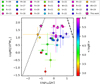 |
Fig. 1 Initial mass of the cluster as a function of the half-mass radius. The color bar represents the number of particles. The dashed black line represents the relaxation time, and the dotted black line corresponds to the collision time when both are equal to a time evolution (i.e., age) of τ = 10 Gyr, which we considered as an upper limit for the typical evolutionary times of the clusters. The symbols indicate different simulations: N-body (squares), Monte Carlo (circles), hybrid N-body (diamonds), and this work (star). |
3.2 Initial conditions for MOCCA, and code modifications
Similar to the direct N-body runs, the input parameters that govern stellar and binary evolution prescriptions in MOCCA were set to level C as described in Kamlah et al. (2022a) and Appendix A. For these runs, the overall time step in MOCCA was reduced to 0.02 Myr. Given the short central relaxation time of this dense model, the smaller time step allowed us to better resolve the evolution and growth of the VMS. Additionally, it enabled a more accurate capture of mass segregation and the effects of mass loss on the cluster’s evolution. In the MOCCA run, three-body binary formation (3BBF) was specifically disabled for the VMS only when its mass exceeded 500 M⊙ to allow for a more accurate comparison with N-body results. This modification was necessary because, in M OCCA, a star in a binary is not allowed to undergo two-body hyperbolic collisions. If the VMS is in a binary, it can only grow through collisions or mergers during binary-single and binary-binary encounters. With 3BBF enabled for the VMS, it frequently formed a binary and remained bound for extended periods, preventing it from growing through two-body collisions. As a result, in the simulation with 3BBF enabled, the VMS reached a mass of only 35 000 M⊙ within 4.5 Myr, significantly limiting its growth compared to the direct N-body simulation. This restriction is a limitation of MOCCA from which NBODY6++GPU is free, where two-body collisions can still occur even if the VMS is part of a binary system. By disabling 3BBF for the VMS in MOCCA, we allowed it to undergo two-body collisions more freely, leading to a growth rate much closer to that observed in NBODY6++GPU. This adjustment was crucial for achieving a more consistent comparison between the two simulation methods. Recent work by Atallah et al. (2024) on 3BBF showed that in interactions with a large mass ratio, 3BBF favors pairing the two least massive bodies. Given these findings, disabling 3BBF for the VMS in MOCCA may not be an unreasonable approach, as it prevents the VMS from being preferentially locked into a binary with a much lower-mass companion, thereby allowing for more efficient growth through collisions.
4 Results
In this section we present and discuss the evolution of the star cluster, the dynamics of the VMS, its evolution due to collisions, their impact on rejuvenation and the formation of an IMBH.
4.1 Dynamical star cluster evolution, the evolution of a VMS, and formation of an IMBH
We dynamically evolve our system for 5 Myr, when already a VMS had formed and evolved into an IMBH. However, relaxation processes are still relevant, since mass segregation takes place much faster than the global half-mass relaxation time given above, with a difference of three order of magnitude (Khalisi et al. 2007).
Figure 2 shows the average mass of the cluster inside the Lagrangian radii (top) and the Lagrangian radii (bottom), which shows the different evolution of shells from the inner to the outer regions. In our model, the star cluster evolves rapidly in the innermost regions (1%), where strong mass segregation triggers an early core collapse. The 10% Lagragian radii start to decrease after 3 Myr of evolution. The 30%, 50%, 70% and 90% Lagrangian radii show the smooth expansion of the cluster; Until around 4.69 Myr (solid lines) and 4.48 Myr (dashed lines) when the IMBH is formed, in N-body and MOCCA simulations, respectively. For the innermost mass shell (1%) we can follow the formation of the VMS, as its mass is getting larger than the corresponding Lagrangian shell’s mass. Notably, the VMS reaches a mass of Mvms ≥ 1000 M⊙ at time 0.18 Myr (N-body simulation) and 0.22 Myr (MOCCA simulation).
Figure 3 shows the cumulative mass of the escapees during the simulation. In the first million years, the cumulative escaped mass is approximately 4000-5000 M⊙, increasing to around 20 000 M⊙ after 5 Myr. N-body and MOCCA simulation show reasonable agreement. The figure also presents the total number of collisions, which amounts to 22010. Of these, 91.6% involves the VMS/IMBH, these collisions can be divided into binary collisions (45.1%) and hyperbolic collisions (46.5%). Binary collisions are more frequent when the VMS mass exceeds 1 000 M⊙ at time 0.18 Myr. In contrast, hyperbolic collisions become more frequent as the VMS grows in size, reaching a radius larger than 1 000 R⊙ at time 3.36 Myr. For the MOCCA simulation, we do not distinguish between binary and hyperbolic collisions, as the code does not explicitly track stellar orbits. Some collisions may involve stars that were gravitationally bound to the VMS, but confirming this would require reconstructing stellar orbits from snapshots using their instantaneous positions, velocities, and the local gravitational potential, which is challenging due to the limited temporal resolution. Consequently, we report only the total number of collisions (16 103 in 5 Myr), of which 65.6% involve the VMS/IMBH. Despite this limitation, the results from the two codes agree well.
Figure 4 compares the NBODY6++GPU and MOCCA simulations, showing the time evolution of the masses of escapees from the cluster (top panels) and secondary stars involved in collisions with the VMS/IMBH (bottom panels). The left panels display the N-body results, and the right panels show the MOCCA results. The color scale represents the local point density of events, with yellow regions indicating higher concentrations of recorded data points. In both simulations, low-mass stars (typically ≲1 M⊙) dominate the population of escapees. The N -body simulation shows two prominent epochs of escapee activity: an extended early phase over the first ~2 Myr, followed by a shorter but more intense burst near the time of IMBH formation at 4.69 Myr. In contrast, the MOCCA simulation exhibits a smoother and more gradual decline in escapee activity over time, with a modest peak near 4.48 Myr corresponding to IMBH formation.
The lower panels show the masses of stars colliding with the VMS/IMBH. MOCCA displays a broader and more uniform spread across the stellar mass range from the start of the simulation, while the N-body simulation shows occasional high-mass collisions (with m ≳ 10 M⊙), though these are relatively sparse. In both simulations, most collisions involve low-mass stars. However, these frequent low-mass mergers contribute less significantly to the final VMS/IMBH mass (see also Fig. 5). The N-body simulation shows a brief dip in the number of secondary stars involved in collisions around 1.68 Myr, lasting approximately 0.1 Myr. This feature coincides with the formation of a hard binary between the VMS and a main-sequence star (see Fig. 7). Subsequent three-body interactions lead to enhanced escape rates. Toward the end of the simulation, the IMBH sequentially forms two hard binaries with ~2 M⊙ MS stars, which explains the observed drop in further collisions.
Figure 5 shows histograms of the number of collisions (top panels) and the cumulative mass of the secondary star colliding with the VMS/IMBH (bottom panels). The N-body results are shown in the left panels, while the MOCCA results are shown in the right panels, the histogram mass ranges <0.1,0.1-1, 1-10, 10100 and >100 M⊙. The number of collisions for N-body are 2057, 14 525, 2525, 923, 95, while for MOCCA are 1053, 7797, 2273, 1570, 74, for the first two mass ranges, N-body has about twice as many collisions as MOCCA, for the mass range 1-10 M⊙ the number of collisions is about 300 more in N-body, while for the next mass range 10-100 M⊙ it is higher for MOCCA, about 600 more collisions. Finally, for the last mass range >100 M⊙ the number of collisions is slightly large in the N-body simulation. In the case of N-body simulations where it is possible to distinguish between binary (red bars) and hyperbolic (blue bars) collisions, we can observe that hyperbolic collisions contribute slightly more to the VMS formation for the mass range <0.1, 0.1-1 M⊙. The mass range 1-10 M⊙ shows almost the same number of collisions, however, binary collisions contribute slightly more to the VMS mass, while binary collisions contribute quite a bit more to the VMS formation for the mass range 10-100, and > 100 M⊙. Both codes show that most of the collisions come from stars in the mass range 0.1-1 M⊙. The largest mass contribution to the VMS comes from stars in the mass range 10-100 M⊙, however. For MOCCA, the mass contribution is 4.41 × 10⁴ M⊙, and for N-body, it is 3.35 × 10⁴ M⊙ (2.73 × 10⁴ M⊙ from binary collisions (cyan bar) and 6.34 × 10³ M⊙ from hyperbolic collisions (magenta bar)). The second largest mass contribution to the VMS comes from the mass range >100 M⊙ with 9.46 × 10³ M⊙ in MOCCA, with 1.26 × 10⁴ M⊙ in N-body, and with 1.17 × 10⁴ and 914.19 M⊙ from binary and hyperbolic collisions, respectively. For the lower mass ranges <0.1, 0.1-1 and, 1-10 M⊙ the VMS mass contribution in the same order is 94.49, 2.59 × 10³ M⊙ and, 8.18 × 10³ M⊙ for MOCCA, while for N-body it is 184.01, 4.69 × 10³ M⊙ and, 6.80 × 10³ M⊙, for this mass ranges the VMS mass contribution from binary and hyperbolic collisions is quite similar.
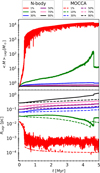 |
Fig. 2 Average mass in each Lagrangian shell 〈M〉Lagr[M⊙] (top) and the Lagrangian radii RLagr [pc] (bottom), both normalized by the cluster mass at the beginning of the simulation. We show the N-body and MOCCA results for the Lagrangian radii. The two plot show the shell representing 1%, 10%, 30%, 50%, 70%, and 90%. The differences between the Lagrangian radii in the N-body and MOCCA simulations arise from how escaping stars are treated. In the N -body simulations, stars with positive energy are not immediately removed from the system; instead, they remain until they cross a boundary set at ten times the half-mass radius. These stars are still included in the calculation of Lagrangian radii, which affects the results compared to MOCCA. |
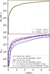 |
Fig. 3 Cumulative mass of escapees (top panel) and cumulative number of collisions (bottom panel). The total number of collisions is represented by a solid black line (N-body) and solid magenta line (MOCCA), while collisions involving the VMS are shown with a dot-dashed purple line (N-body) and solid cyan line (MOCCA). The binaries involving the VMS are shown with a dotted red line, and hyperbolic collisions with the VMS are shown by a dashed blue line. |
4.2 N-body results: VMS evolution and IMBH formation
In our N-body simulation, several collisions along the simulation to build up a VMS with a mass of 56 996.91 M⊙, eventually collapsing and forming an IMBH with a mass of 51 625.99 M⊙ at time 4.69 Myr.
Figure 6 shows the scatter of the position relative to the star cluster’s density center of the VMS (and IMBH thereafter), ξVMS,IMBH [pc], and the speed of the VMS (and IMBH, when formed), vVMS,IMBH [km s−1]. Initially, the star with a mass of 130.58 M⊙, which later becomes the VMS, is located at 0.088 pc from the center, sinking with a velocity of 32.9 km s−1. After around 100 years, it moves closer to the center at 0.061pc, while its velocity increases nearly threefold to 99.7 km s−1. A few hundred years later, it reaches a velocity of 165.1 km s−1 at a position of 0.018 pc. This rapid infall toward the center is driven by the high cluster density, but the VMS position and velocity oscillations are consistent with the orbital time. After two collisions with MS stars (i.e., stars with a fraction of a solar mass), the first significant collision occurs with a star of mass 54.89 M⊙ following a binary interaction. At this point, the star is at 0.006 pc. As shown in the figure, the motion of the VMS, in terms of position and velocity, first aligns with the expectations of mass segregation (steady decrease in distance to the center and a velocity profile that initially rises before declining) and later transitions to Brownian motion. At 1.68 Myr a hard binary system forms between the VMS and an MS star. Figure 7 shows the semimayor axis and eccentricity of the hard binary formed between the VMS with a mass of 28 891 M⊙ and a secondary star with a mass of 75 M⊙. Both stars are tightly bound due to their small average distance (<3 AU), they have an elliptical orbit, this dynamical interaction lasted about 0.1 Myr. The binary system have a higher binding energy than the kinetic energy of the surrounding stars, which eventually gain kinetic energy, increasing their velocity. The latter reduces the probability of low-velocity stars that could collide with the VMS. Throughout the simulation, the velocity and position of the VMS remain nearly constant, fluctuating around an average value of about 10−3 pc, while the velocity remains in moderate motion, at a few kilometers per second.
As supported by the theoretical expectations discussed in previous sections, the VMS growth in the N-body simulation occurs on a short time-scale. The VMS original progenitor passes from an initial mass of 130.58 M⊙ to exceed 103 M⊙ after only 0.18 Myr through 17 collisions, further reading >5000 M⊙ in a time 0.29 Myr. The VMS continues its growth for 0.48 Myr through several collisions until reaching more than 104 M⊙, naturally, the size of the VMS also increases having 71.13 R⊙, the continued collisions allow a strong rejuvenation of the star, which has an effective age 0.23 Myr. Lately, around 1.0 Myr the VMS has a mass, effective age, and radius of 1.9 × 10⁴ M⊙, 0.54 Myr, and 80.75 R⊙, respectively. The evolution of the mass, radius, and age of the VMS is shown in the top, middle, and bottom left panels of Fig. 8.
At 2 Myr, the VMS has a mass of 3.1 × 10⁴ M⊙, with a radius 146.24 R⊙ and effective age 1.21 Myr, the hard binary system formed at 1.68 Myr in the N-body simulation prevents the VMS from experiencing further collisions, thus leads to a VMS with about 4000 M⊙ less mass than the VMS obtained in MOCCA simulation, that has a mass of 3.5 × 10⁴ M⊙ at the same simulation time, 1 Myr later the N-body VMS reaches a mass, radius, and effective age of 4.3 × 10⁴ M⊙, 507.24 R⊙ and 1.77 Myr, respectively. The N-body VMS still have less mass than the MOCCA VMS which have a mass 4.52 × 10⁴ M⊙ at 3 Myr.
The hydrogen burning phase is set to end in 2.9 Myr, according to the SSE/BSE prescription Hurley et al. (2000, 2002a, 2005). After the VMS reaches this point, it should start burning helium. At 4.67 Myr the VMS has a mass of 5.7362 × 10⁴ M⊙, with a radius of 1.9 × 10⁵ R⊙ and effective age of 2.91 Myr. At this stage, the VMS becomes a helium main sequence (HeMS; or type 7 in SSE/BSE by Hurley et al. 2000, 2002a, 2005) star with a radius of 171 R⊙. During this helium phase, the VMS experiences three collisions with MS stars within 0.02 Myr before naturally collapsing into an IMBH. This process may result in mass loss of about 10 % due to neutrino emission (Fryer et al. 2012; Kamlah et al. 2022a), leading to a mass of 51 625.99 M⊙ at time 4.69 Myr. Finally, the IMBH undergoes additional collisions, accreting 50% of the stellar companion (Rizzuto et al. 2021), reaching a final mass of 51 661.21 M⊙ by the end of the simulation.
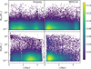 |
Fig. 4 Top panels: mass of each escaping star. Bottom panels: mass of the secondary star before it collides with the VMS for hyperbolic and binary collisions. The color bar represents the density distribution of the stars. |
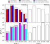 |
Fig. 5 Histograms showing the contribution of colliding stars to VMS formation, divided into binary, hyperbolic, and total collisions. The mass ranges are < 0.1 M⊙, 0.1-1 M⊙, 1-10 M⊙, 10-100 M⊙, and > 100 M⊙. Results are shown for the N-body simulation (left column) and the MOCCA simulation (right column). The top panel displays the number of collisions, and the bottom panel shows the cumulative mass contributed by these collisions. |
4.3 MOCCA results: VMS evolution and IMBH formation
In the MOCCA simulation, the star that eventually grows into a VMS has an initial mass of 130.6 M⊙ and is initially located at a distance of 0.088 pc from the center of the cluster. Within 0.15 Myr, this massive star undergoes four collisions with low mass stars, slightly increasing its mass to approximately 132 M⊙. For a brief period between about 0.18 Myr and 0.21 Myr, the VMS is part of a binary system. At 0.182 Myr, the VMS first forms a binary with a 72.4 M⊙ star due to 3BBF. Shortly after, at 0.183 Myr, this companion is replaced by a 124 M⊙ star in an exchange encounter. Following several flyby interactions, the VMS and its binary companion merge during a binary-single interaction at 0.186 Myr. The VMS subsequently forms another binary, first with a 72.4 M⊙ star, then with a 68 M⊙ star, and later with a 174 M⊙ star. The latter also merges with the VMS in a binary-single interaction at around 0.21 Myr, following several flyby encounters. At this stage, the VMS is located at a distance of approximately 3 × 10⁻⁴ pc from the cluster center. By 0.212 Myr, its mass exceeds 500M⊙ following a collision with a 121.8 M⊙ star, with which it was also briefly in a binary system. As described in Sect. 3.2, from this point onward, we disable 3BBF for the VMS. Its mass continues to increase rapidly as it undergoes runaway collisions with other MS stars in the cluster center. By 0.23 Myr, the VMS mass reaches 1000 M⊙, and by 0.34 Myr, it exceeds 5000 M⊙. The growth of the VMS in MOCCA is shown in the top-right panel of Fig. 8.
During these early stages of VMS growth, collisions with other VMSs also strongly rejuvenate it. At 0.34 Myr, when its mass reaches 5000 M⊙, its effective age is only 0.068 Myr, and its radius is approximately 68 R⊙. By 0.51 Myr, the VMS mass surpasses 104 M⊙, at which point its effective age is 0.17 Myr, and its radius is 71.5 R⊙. The VMS continues its rapid growth, reaching 2.1 × 10⁴ M⊙ by 1 Myr. By this time, the cumulative number of collisions involving the VMS is approximately 3815 (see Fig. 3). As the mass ratio of these collisions decreases with increasing VMS mass, its effective rejuvenation per collision also weakens. At 1 Myr, its effective age is 0.468 Myr. The evolution of the VMS’s effective age on the MS is shown in the bottom-right panel of Fig. 8.
By 2 Myr, the VMS reaches a mass of 3.56 × 10⁴ M⊙, with an effective age of 1.1 Myr and a radius of 131 R⊙. Up until this point, the VMS has undergone more than 6793 collisions. Between 2 Myr and 3 Myr, its growth slows, and by 3 Myr, it reaches a mass of 4.59 × 10⁴ M⊙ with an effective age of 1.77 Myr. This corresponds to approximately 61% of the MS lifetime of the VMS, which is set to 2.91 Myr in the SSE/BSE prescriptions used in NBODY6++GPU and MOCCA. As the VMS ages, its radius increases, reaching 523 R⊙ at 3 Myr. The evolution of the VMS’s radius is shown in the middle-right panel of Fig. 8.
At 4.477 Myr, the VMS reaches a mass of 5.38 × 10⁴ M⊙, with a radius of 1.9 × 10⁵R⊙ and an effective age of 2.91 Myr, marking the MS turn-off time for the VMS. By this point, it has undergone 10 322 collisions. After this stage, the VMS evolves into a helium main sequence star (HeMS; type 7 in SSE/BSE) with a radius of 165 R⊙. Between 4.477 Myr and 4.485 Myr, the HeMS VMS undergoes approximately 15 additional collisions with lower-mass stars, reaching a final mass of 5.384 × 10⁴ M⊙. As the mass ratios in these collisions are extremely small, no rejuvenation is applied. At 4.485 Myr, the VMS evolves into an IMBH with a mass of 4.845 × 10⁴ M⊙. This IMBH then continues to grow through collisions, mostly with other stars, assuming that 50% of the stellar mass is accreted by the IMBH in each collision. By 5 Myr, it reaches a mass of 4.984 × 10⁴ M⊙.
The short duration of the HeMS phase in the evolution of the VMS is a result of the inverse dependence of the HeMS lifetime (tHeMS) on stellar mass (see Eq. (79) in Hurley et al. 2000). As discussed in Sect. 4.2, the amount of mass lost due to neutrinos when the VMS transitions into an IMBH is set to 10%, consistent with the default assumptions in NBODY6++GPU1. We also performed an alternative MOCCA run in which the HeMS lifetime of the VMS was extended to 0.3 Myr. In this case, the VMS remained on the HeMS long enough to undergo a collision with a 53.3 M⊙ stellar mass BH present in the cluster. Although the mass ratio of this merger was extremely small, if the VMS was allowed to change its stellar type following the collision, the BH was treated as absorbing 50%2 of the VMS mass. This alternative treatment led to the formation of an IMBH with a mass of 2.6725 × 10⁴ M⊙.
Overall, the MOCCA evolution of the VMS mass, radius, and effective age in the simulation presented here is in good agreement with the NBODY6++GPU results, as shown in Fig. 8. The mass distribution and number of stars that collide with the VMS are shown in Fig. 5, where the top right panel highlights that the total number of collisions involving the VMS is lower in MOCCA compared to the direct N-body simulation (top left panel). This results in less efficient rejuvenation, allowing the VMS to reach the end of its main-sequence lifetime and evolve into an IMBH slightly earlier (by about 0.2 Myr) than in the N-body run. Despite the reduced number of collisions, the final VMS mass at the time of IMBH formation is only 3500 M⊙ smaller in MOCCA, due to the fact that no mass is lost during MS collisions in this simulation.
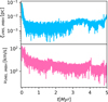 |
Fig. 6 Temporal evolution of the position of the VMS relative to the star cluster density center, ξVMS,IMBH, and the speed of the VMS relative to the star cluster density center, νVMS,IMBH. |
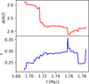 |
Fig. 7 Temporal evolution of a hard binary system during between 1.68 and 1.80 Myr. This binary has the primary star as the VMS, with a mass of 28 891 M⊙ and a secondary star with a mass of 75 M⊙. This interaction lasts approximately 0.1 Myr. The top panel shows the semimajor axis, while the bottom panel shows the eccentricity. |
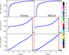 |
Fig. 8 Evolution of the VMS (and IMBH thereafter) over time. Top panel: mass of the VMS/IMBH, MVMS,IMBH [M⊙]. Middle panel: stellar radius of the VMS/IMBH, RVMS,IMBH [R⊙] (logarithmic scale). Bottom panel: effective age of the VMS during its main-sequence phase, AVMS,IMBH [Myr]. |
5 Summary, conclusions, and outlook
We investigated the formation of VMSs through stellar mergers, using direct N-body and MOCCA simulations. To better follow the evolution and growth of a VMS in these models, several improvements were made to the standard stellar evolution routines in NBODY6++GPU and MOCCA. These included updates to the treatment of stellar radius evolution, rejuvenation, and close encounter prescriptions. We note that the prescriptions implemented here represent reasonable extrapolations of standard SSE/BSE stellar evolution models (Hurley et al. 2000, 2002a, 2005; Kamlah et al. 2022a); however, the internal structure and thermal state of VMS formed through stellar collisions remain to be established and require further refinement. Our simulations demonstrate the growth of a VMS through successive mergers, reaching several tens of thousands of solar masses. The formation of such a massive object through a purely collisional pathway highlights the potential importance of this channel in the formation of IMBHs and SMBH seeds. This dual approach allows us to test the robustness of the VMS formation channel across methods with different computational schemes and resolution limits. We note that the MOCCA results required some adjustments to achieve consistency with the NBODY6++GPU simulations. In particular, the timestep was reduced to better capture the mass segregation time of massive stars. Without this change, a VMS would still have formed and reached a comparable final mass to the N-body run, but its growth would be delayed by ≈0.2 Myr. In addition, 3BBF was disabled for the VMS once it exceeded 500 M⊙. With 3BBF enabled, the VMS quickly forms a binary and is prevented from undergoing two-body collisions, reaching only ~35 000 M⊙ at 4.5 Myr. In contrast, with 3BBF disabled, the collisional growth of the VMS proceeds at a rate consistent with the direct N-body result. These points are discussed in more detail in Sect. 3.2.
5.1 Theoretical considerations and simulation constraints
The formation of VMSs through runaway collisions in dense star clusters was first proposed by Begelman & Rees (1978), Rees (1984), and Lee (1987) using simple analytical models. This scenario was later explored using Fokker-Planck and Monte Carlo methods by Quinlan & Shapiro (1990); Gürkan et al. (2004); Freitag et al. (2006a,b) and Sharma & Rodriguez (2025), and more recently through direct N-body simulations by Vergara et al. (2023). In clusters with a larger number of particles, dynamical equilibrium is typically reached before thermodynamic equilibrium. As a result, such systems require longer times to undergo core collapse and reach Spitzer instability without significant expansion due to relaxation processes (Spitzer 1987). Our results support the existence of a critical mass threshold for the formation of massive objects via collisions, as previously suggested by Vergara et al. (2023, 2024). Our simulations push into an uncharted regime of extremely high central density and particle number, testing the runaway collision scenario under extreme but plausible cluster conditions.
The high central density of the clusters in our models (> 107 M⊙ pc−3) leads to an elevated stellar collision rate, significantly higher than that in typical observed globular clusters. Consequently, the time between successive collisions becomes much shorter than the thermal timescale of the VMS. This rapid succession of collisions prevents the VMS from reaching thermal equilibrium between impacts, potentially causing it to expand beyond its equilibrium radius, which may, in turn, alter its collision cross section and affect the likelihood and nature of subsequent encounters. The physical and thermodynamical structure of such a VMS lies in a largely unexplored regime, and it may experience significant mass loss through repeated collisions and strong stellar winds, both of which can affect its growth in radius and mass (Dale & Davies 2006; Suzuki et al. 2007). As a result, our simulation likely provides an optimistic upper limit on the achievable VMS mass under such conditions.
Repeated collisions also rejuvenate the VMS, delaying its natural evolution toward collapse into a BH. VMSs may be important contributors to cosmic hydrogen and helium reionization, a process that depends sensitively on stellar wind mass-loss rates and metallicity (Vink et al. 2021; Sander & Vink 2020). In our models, we adopt a relatively high metallicity of Z = 0.01, which enhances wind-driven mass loss and makes VMS formation more difficult compared to lower-metallicity environments. Despite this, the VMS forms rapidly enough that winds do not inhibit its growth, owing to the assumption that the star returns to thermal equilibrium following each collision. Between the two codes, the higher collision rate in the N-body run leads to more frequent rejuvenation and prolongs the main-sequence lifetime of the VMS compared to the MOCCA run. The stellar wind prescriptions in the two simulations are based on the works of Vink et al. (2001), Vink & de Koter (2002, 2005), and Belczynski et al. (2010). As the VMS evolves into the helium-burning phase, it experiences stronger but shorter-lived wind episodes. For this phase, we adopt a luminosity-dependent wind recipe following Sander & Vink (2020). However, since the helium main-sequence lifetime is relatively short (~0.01 Myr) for the VMS in these runs, there is no significant mass loss due to winds during this evolutionary stage. In future work, we plan to implement a more refined mass-luminosity relation to improve the modeling of VMS evolution and feedback.
The early and rapid mass gain in our models is essential; had the VMS grown more slowly, stellar winds at Z = 0.01 would likely have halted its development, preventing IMBH formation. However, this outcome also depends on how strongly the VMS deviates from thermal equilibrium after collisions, as larger radii could enhance the stellar collision rate and potentially compensate for wind-driven mass loss. Furthermore, the IMBH forms through the direct collapse of the VMS, with an assumed mass loss of approximately 10% due to neutrino emission (Fryer et al. 2012; Kamlah et al. 2022a). However, the exact amount of mass lost, if any, during the transition from an evolved star to a BH remains uncertain.
VMS formation at high metalicities (Z = 0.01-0.02) has also been investigated using smoothed-particle hydrodynamics (SPH) simulations with ASURA-BRIDGE (Fujii et al. 2024a).
These studies model dense clusters with central densities of 106−109 M⊙ pc−3 and show that IMBHs with masses exceeding 4000 M⊙ can form within approximately 1.5 Myr (Fujii et al. 2024b). The inclusion of gas in these models contributes to the higher central densities and enhances the conditions for runaway collisions and rapid VMS growth. Unlike our gas-free N-body and Monte Carlo models, these simulations demonstrate how gas inflows can further support the VMS formation channel. Nevertheless, our results show that even in purely stellar systems, rapid VMS formation is feasible under extreme initial conditions.
If we interpret runaway stellar collisions as analogous to gas accretion, we can compare our results to models of accreting stars (Haemmerlé et al. 2018; Herrington et al. 2023). In particular, we focus on models with an accretion rate of ~0.01 M⊙ yr−1, which is comparable to the effective rate at which our VMS gains mass through mergers. These models predict that accreting stars expand to radii of ~104 R⊙ along the Hayashi track. Notably, Herrington et al. (2023) terminate their simulations at central hydrogen depletion. The VMS in our simulations reaches a radius comparable to those found in these accreting-star models. Since stellar radius is an important parameter influencing collision rates and outcomes, the agreement between our VMS radii and those predicted in accretion models supports the plausibility of the VMS growth we observe. However, the internal structure of a VMS built through collisions may differ significantly from that of an accreting MS star. In particular, collisional VMSs may develop a dense core with an extended, dilute envelope, potentially reducing the efficiency of further mass buildup by lowering the effective collision cross section. This structural difference adds uncertainty when interpreting the final VMS mass in our simulations.
Furthermore, Martinet et al. (2023) present stellar evolution models computed with the GENEC code (Eggenberger et al. 2008) for metallicity Z = 0.014, including rotating and nonrotating stars with initial masses of 180, 250, and 300 M⊙. These models yield main-sequence lifetimes of approximately 2.2-2.6 Myr. In comparison, the SSE models by Hurley et al. (2000), which we use in our simulations, give a main-sequence lifetime of 2.9 Myr at Z = 0.01. This agreement suggests that the stellar evolution prescriptions adopted in our simulations are consistent with more detailed stellar evolution models, lending credibility to our estimates of VMS lifetimes and their impact on subsequent cluster evolution.
The radiative efficiency of stellar winds from VMSs could play an important role in the chemical enrichment of star clusters. This process has been proposed as a potential mechanism for the formation of multiple stellar populations (MSPs; Gieles et al. 2018, 2025). Recent high-resolution hydrodynamic simulations have provided the first detailed insights into VMS self-enrichment in massive clusters, highlighting its relevance for MSP formation. Stellar winds enriched with elements such as Na, Al, and N can be retained within the cluster and contribute to the formation of chemically distinct stars within just a few million years (Lahén et al. 2024). In addition to stellar winds, stellar mergers offer an alternative pathway for MSP formation. In dense clusters where mergers are more frequent, these events can eject chemically enriched material into the surrounding gas. This material - whether expelled through dynamical interactions, explosions, or fusion-driven outflows - can lead to the formation of new stars with distinct chemical compositions (Wang et al. 2020b). Recent observational studies have also revealed detailed kinematic differences between stellar populations, showing that second-generation stars tend to rotate more rapidly and are more centrally concentrated than first-generation stars (Dalessandro et al. 2024). These findings provide further motivation for detailed modeling of early cluster enrichment scenarios involving VMSs, especially in young massive clusters forming at high redshift.
5.2 Observational context for VMS formation at high redshift
Observing massive, compact, and low-metallicity star clusters around the time of core collapse remains extremely challenging. However, high-redshift galaxies are widely expected to form such clusters efficiently due to their high gas fractions and low metallicities (e.g., Tacconi et al. 2010), as well as their clumpy substructures that favor gravitational fragmentation and rapid star formation (e.g., Devereaux et al. 2024). These conditions closely mirror those adopted in our simulations, reinforcing the plausibility of early VMS formation via runaway stellar collisions. We note that the majority of massive stars observed have masses of approximately 100-300 M⊙ (Doran et al. 2013; Keszthelyi et al. 2025), stars with masses above this limit remain purely theoretical.
Recent observations using strong gravitational lensing have begun to probe star-forming clumps and stellar clusters in high-redshift galaxies. For example, Claeyssens et al. (2023) analyzed clump populations in galaxies at z = 1-8.5, identifying halfmass radii ranging from a few to several tens of parsecs. They also found evidence of a mass-size scaling relation that may lie above the local relation (Brown & Gnedin 2021), although the observed population is likely biased toward more massive and extended systems. Nevertheless, extremely compact clusters are still expected to form in high-density environments, even if they remain observationally elusive.
From a theoretical standpoint, the Toomre instability criterion implies that the typical cluster size should scale inversely with the square root of the gas surface density, i.e.,  (Toomre 1964). This suggests that star clusters formed in gas-rich, high-redshift galaxies should be significantly more compact than their local counterparts - a trend also supported by simulations and nearby observations (Choksi & Kruijssen 2021). Reinforcing this, Adamo et al. (2024) recently reported several compact clusters at z ~ 10 with effective radii below one parsec and enhanced surface densities compared to local analogues. These findings support the idea that extremely dense clusters, such as those used in our models, could plausibly form in the early Universe. However, our models do not include residual gas, which could remain trapped in such compact systems and influence early dynamical evolution and VMS formation.
The presence of such dense clusters may also be required to explain chemical signatures observed in some high-redshift systems. Notably, the candidate galaxy GN-z11 at z = 10.6 (Bouwens et al. 2010; Tacchella et al. 2023; Nagele & Umeda 2023; Maiolino et al. 2024) exhibits an unusually high nitrogen-to-oxygen abundance ratio, with log10(N/O) > -0.25 - a value roughly four times the solar ratio (Cameron et al. 2023). Similar enhancements have been reported in other high-z sources (Marques-Chaves et al. 2024). Rapidly rotating Pop-III stars have been suggested as a potential source of nitrogen enrichment (Tsiatsiou et al. 2024; Nandal et al. 2024). Additionally, high nitrogen abundances could originate from hydrogen-burning nucleosynthesis in VMS formed via runaway stellar collisions (Charbonnel et al. 2023). Our results, which show VMS growth within a few million years support this scenario by demonstrating that VMSs can form early and potentially enrich their surroundings before core collapse.
Compact massive clusters may also form during major galaxy mergers, particularly at high redshift where galaxies are more gas-rich and metal-poor. Mergers can trigger large-scale inflows of gas, leading to starbursts and the formation of dense stellar systems containing >104 to 106 stars (Renaud et al. 2015). While nearby merging systems like the Antennae galaxies have near-solar metallicities (Fall et al. 2005), similar processes occurring in early galaxies (e.g., Pettini et al. 1997) could create the ideal conditions for VMS formation. This has been demonstrated in simulations by Lahén et al. (2019, 2020b,a), where massive clusters with masses >105 M⊙ formed in the aftermath of gasrich dwarf galaxy mergers. These simulated clusters are broadly consistent with the initial conditions explored in our models, reinforcing the relevance of our results for understanding early IMBH seed formation in the cosmological context.
5.3 Outlook: Observational signatures and future tests
Tidal disruption events (TDEs) represent a promising observational signature of massive black holes (BHs), including those that may have formed via the collisional pathways we modeled. These events occur when a star passes sufficiently close to a BH to be partially or fully disrupted and accreted, and they produce luminous flares across the electromagnetic spectrum (Hills 1975; Rees 1988). TDEs are associated with the so-called loss cone, which is a region in phase space that contains stellar orbits that bring stars close enough to be disrupted (Chandrasekhar 1942). In spherical systems, this region is rapidly depleted, and its replenishment through two-body relaxation is typically slow (Broggi et al. 2024). Although TDEs can contribute to BH growth, our simulations concluded shortly after IMBH formation, and longer-term dynamical evolution that includes loss-cone refilling remains a key area for future study.
In the regime of the empty loss cone, where stellar orbits rarely intersect the tidal BH radius, BH growth stalls unless it is aided by additional processes such as gas accretion or compact object mergers (e.g., Stone & Metzger 2016; Ryu et al. 2020a,b,c; Stone et al. 2020). One particularly intriguing channel involves the gradual inspiralling of compact remnants (neutron stars or stellar mass BHs) around an IMBH. This class of events is known as extreme mass-ratio inspirals (EMRIs; Hils & Bender 1995). EMRIs are shaped by dynamical friction, relativistic precession, and tidal forces, and they represent a key gravitational wave (GW) signature of IMBHs in dense star clusters (Broggi et al. 2022). Our results demonstrated early IMBH formation via runaway collisions and suggest that these GW sources might appear much earlier in cosmic history than traditionally assumed.
Crucially, these processes are not only theoretically predicted, but are increasingly accessible to observation. TDEs produce luminous flares that are observable with facilities such as the Hubble Space Telescope (HST; Leloudas et al. 2016) and the Neil Gehrels Swift Observatory (Swift; Brown et al. 2016). On the other hand, mergers involving compact objects (including EMRIs) are detectable with current GW observatories such as LIGO, Virgo, and KAGRA (Abbott et al. 2024), and will be prime targets for future space-based missions like LISA (Amaro-Seoane et al. 2017; McCaffrey et al. 2025) and the Einstein Telescope (ET; Punturo et al. 2010).
Complementary electromagnetic observations will further aid in testing the predictions of our collisional IMBH formation scenario. The upcoming JASMINE mission will offer ultraprecise astrometry of the nuclear star cluster in the Milky Way, which will enable dynamical BH mass measurements. The Extremely Large Telescope (ELT), with its near-infrared imager MICADO, will be capable of resolving the sphere of influence of BHs at distances up to twice that of JWST (Davies et al. 2018). The JWST has already revealed a population of compact red sources (the so-called little red dots) that are interpreted as dusty supermassive BHs (SMBHs) or obscured star-forming galaxies (Kokorev et al. 2024; Akins et al. 2025; Matthee et al. 2024; Napolitano et al. 2025). The BH-to-stellar mass ratio of these high-redshift objects are unusually high and higher by up to two orders of magnitude than those seen locally (Goulding et al. 2023; Scoggins et al. 2023; Übler et al. 2024; Furtak et al. 2024; Juodžbalis et al. 2024). These findings suggest the presence of overmassive BHs in the early Universe and challenge conventional models of BH seed formation.
Our results offer a complementary explanation, that is, the formation of massive BH seeds via runaway stellar collisions in dense clusters, followed by early collapse into IMBHs. This purely collisional pathway may help reconcile observations of overmassive BHs at high redshift with theoretical models, particularly if dense star clusters like those in our simulations were common in the early Universe. Future multimessenger observations that combine GWs and electromagnetic signatures will be essential for distinguishing between different IMBH formation channels and testing the predictions of this work.
Data availability
The underlying data, including the initial model used in this work, as well as the output and diagnostic files from both the Nbody6++GPU and MOCCA simulations, are publicly available at https://doi.org/10.5281/zenodo.15283075. The Nbody6++GPU code version that includes the level C stellar evolution prescriptions (Kamlah et al. 2022a) is publicly available. The McLuster version used to generate the initial conditions is also publicly available as described in Leveque et al. (2022a,b).
Acknowledgements
MCV acknowledges funding through ANID (Doctorado acuerdo bilateral DAAD/62210038) and DAAD (funding program number 57600326). Furthermore, acknowledges to the International Max Planck Research School for Astronomy and Cosmic Physics at the University of Heidelberg (IMPRS-HD). AA acknowledges support for this paper from project No. 2021/43/P/ST9/03167 co-funded by the Polish National Science Center (NCN) and the European Union Framework Programme for Research and Innovation Horizon 2020 under the Marie Sktodowska-Curie grant agreement No. 945339. For the purpose of Open Access, the authors have applied for a CC-BY public copyright license to any Author Accepted Manuscript (AAM) version arising from this submission. AWHK and RS acknowledge NAOC International Cooperation Office for its support in 2023, 2024, and 2025. RS acknowledges the support by the National Natural Science Foundation of China (NSFC) under grant No. 12473017. This research was supported in part by grant NSF PHY-2309135 to the Kavli Institute for Theoretical Physics (KITP). NH is a fellow of the International Max Planck Research School for Astronomy and Cosmic Physics at the University of Heidelberg (IMPRS-HD). NH received financial support from the European Union’s HORIZON-MSCA-2021-SE-01 Research and Innovation programme under the Marie Sklodowska-Curie grant agreement number 101086388 - Project acronym: LACEGAL. This material is based upon work supported by Tamkeen under the NYU Abu Dhabi Research Institute grant CASS. FFD and RS acknowledge support by the German Science Foundation (DFG, project Sp 345/24-1). PB thanks the support from the special program of the Polish Academy of Sciences and the U.S. National Academy of Sciences under the Long-term program to support Ukrainian research teams grant No. PAN.BFB.S.BWZ.329.022.2023. The work of PB was also supported by the grant No. BR24992759 “Development of the concept for the first Kazakhstan orbital cislunar telescope - Phase I”, financed by the Ministry of Science and Higher Education of the Republic of Kazakhstan. MAS acknowledges funding from the European Union’s Horizon 2020 research and innovation programme under the Marie Sklodowska-Curie grant agreement No. 101025436 (project GRACE-BH, PI: Manuel Arca Sedda). MAS acknowledge financial support from the MERAC foundation. AT is supported by Grants-in-Aid for Scientific Research (grant No. 19K03907 and 24K07040) from the Japan Society for the Promotion of Science. DRGS gratefully acknowledges support by the ANID BASAL project FB21003, as well as via Fondecyt Regular (project code 1201280) and ANID QUIMAL220002. DRGS thanks for funding via the Alexander von Humboldt - Foundation, Bonn, Germany. AH and MG were supported by the Polish National Science Center (NCN) through the grant 2021/41/B/ST9/01191. Xiaoying Pang acknowledges the financial support of the National Natural Science Foundation of China through grants 12173029 and 12233013. TN acknowledges the support ofthe Deutsche Forschungsgemeinschaft (DFG, German Research Foundation) under Germany’s Excellence Strategy -EXC-2094 - 390783311 of the DFG Cluster of Excellence "ORIGINS”. RC is supported in part by the National Key Research and Development Program of China and the Zhejiang provincial top level research support program. AE acknowledge financial support from the Center for Astrophysics and Associated Technologies CATA (FB210003). Computations were performed on the HPC system Raven at the Max Planck Computing and Data Facility, and we also acknowledge the Gauss Centre for Supercomputing e.V. for computing time through the John von Neumann Institute for Computing (NIC) on the GCS Supercomputer JUWELS Booster at Jülich Supercomputing Centre (JSC). Finally, we also acknowledge A. Sander and his team for helpful comments.
References
- Aarseth, S. J. 1985, in Multiple time scales, 377 [Google Scholar]
- Aarseth, S. J. 1999a, PASP, 111, 1333 [NASA ADS] [CrossRef] [Google Scholar]
- Aarseth, S. J. 1999b, CeMDA, 73, 127 [Google Scholar]
- Aarseth, S. J. 2003a, Ap&SS, 285, 367 [Google Scholar]
- Aarseth, S. J. 2003b, Gravitational N-Body Simulations [Google Scholar]
- Aarseth, S. J. 2012, MNRAS, 422, 841 [NASA ADS] [CrossRef] [Google Scholar]
- Aarseth, S. J., Tout, C. A., & Mardling, R. A. 2008, The Cambridge N-Body Lectures, 760 [Google Scholar]
- Abbott, R., Abe, H., Acernese, F., et al. 2024, ApJ, 966, 137 [Google Scholar]
- Adamo, A., Bradley, L. D., Vanzella, E., et al. 2024, Nature, 632, 513 [NASA ADS] [CrossRef] [Google Scholar]
- Ahmad, A., & Cohen, L. 1973, J. Computat. Phys., 12, 389 [NASA ADS] [CrossRef] [Google Scholar]
- Akins, H. B., Casey, C. M., Berg, D. A., et al. 2025, ApJ, 980, L29 [Google Scholar]
- Amaro-Seoane, P., Audley, H., Babak, S., et al. 2017, arXiv e-prints [arXiv:1702.00786] [Google Scholar]
- Arca Sedda, M., Askar, A., & Giersz, M. 2019, arXiv e-prints [arXiv:1905.00902] [Google Scholar]
- Arca Sedda, M., Amaro Seoane, P., & Chen, X. 2021a, A&A, 652, A54 [NASA ADS] [CrossRef] [EDP Sciences] [Google Scholar]
- Arca Sedda, M., Mapelli, M., Benacquista, M., & Spera, M. 2021b, arXiv [arXiv:2109.12119] [Google Scholar]
- Arca-Sedda, M., Rizzuto, F. P., Naab, T., et al. 2021, ApJ, 920, 128 [NASA ADS] [CrossRef] [Google Scholar]
- Arca Sedda, M., Kamlah, A. W. H., Spurzem, R., et al. 2023a, MNRAS, 526, 429 [NASA ADS] [CrossRef] [Google Scholar]
- Arca Sedda, M., Mapelli, M., Benacquista, M., & Spera, M. 2023b, MNRAS, 520, 5259 [NASA ADS] [CrossRef] [Google Scholar]
- Arca Sedda, M., Kamlah, A. W. H., Spurzem, R., et al. 2024a, MNRAS, 528, 5119 [NASA ADS] [CrossRef] [Google Scholar]
- Arca sedda, M., Kamlah, A. W. H., Spurzem, R., et al. 2024b, MNRAS, 528, 5140 [CrossRef] [Google Scholar]
- Askar, A., Bianchini, P., de Vita, R., et al. 2017a, MNRAS, 464, 3090 [Google Scholar]
- Askar, A., Szkudlarek, M., Gondek-Rosinska, D., Giersz, M., & Bulik, T. 2017b, MNRAS, 464, L36 [CrossRef] [Google Scholar]
- Askar, A., Baldassare, V. F., & Mezcua, M. 2023, arXiv e-prints [arXiv:2311.12118] [Google Scholar]
- Atallah, D., Weatherford, N. C., Trani, A. A., & Rasio, F. A. 2024, ApJ, 970, 112 [Google Scholar]
- Bae, Y.-B., Lee, H. M., Kang, G., & Hansen, J. 2017, Phys. Rev. D, 96, 084009 [Google Scholar]
- Banerjee, S. 2021, MNRAS, 500, 3002 [Google Scholar]
- Banerjee, S., Belczynski, K., Fryer, C. L., et al. 2020, A&A, 639, A41 [NASA ADS] [CrossRef] [EDP Sciences] [Google Scholar]
- Begelman, M. C. 2010, MNRAS, 402, 673 [NASA ADS] [CrossRef] [Google Scholar]
- Begelman, M. C., & Rees, M. J. 1978, MNRAS, 185, 847 [NASA ADS] [CrossRef] [Google Scholar]
- Begelman, M. C., Volonteri, M., & Rees, M. J. 2006, MNRAS, 370, 289 [NASA ADS] [CrossRef] [Google Scholar]
- Begelman, M. C., Rossi, E. M., & Armitage, P. J. 2008, MNRAS, 387, 1649 [NASA ADS] [CrossRef] [Google Scholar]
- Belczynski, K., Kalogera, V., Rasio, F. A., et al. 2008, ApJS, 174, 223 [Google Scholar]
- Belczynski, K., Bulik, T., Fryer, C. L., et al. 2010, ApJ, 714, 1217 [NASA ADS] [CrossRef] [Google Scholar]
- Bernini-Peron, M., Marcolino, W. L. F., Sander, A. A. C., et al. 2023, A&A, 677, A50 [NASA ADS] [CrossRef] [EDP Sciences] [Google Scholar]
- Binney, J., & Tremaine, S. 1987, Galactic dynamics [Google Scholar]
- Binney, J., & Tremaine, S. 2008, Galactic Dynamics, 2nd edn. [Google Scholar]
- Björklund, R., Sundqvist, J. O., Singh, S. M., Puls, J., & Najarro, F. 2023, A&A, 676, A109 [NASA ADS] [CrossRef] [EDP Sciences] [Google Scholar]
- Boekholt, T. C. N., Schleicher, D. R. G., Fellhauer, M., et al. 2018, MNRAS, 476, 366 [Google Scholar]
- Bouwens, R. J., Illingworth, G. D., González, V., et al. 2010, ApJ, 725, 1587 [NASA ADS] [CrossRef] [Google Scholar]
- Brem, P., Amaro-Seoane, P., & Spurzem, R. 2013, MNRAS, 434, 2999 [NASA ADS] [CrossRef] [Google Scholar]
- Broggi, L., Bortolas, E., Bonetti, M., Sesana, A., & Dotti, M. 2022, MNRAS, 514, 3270 [NASA ADS] [CrossRef] [Google Scholar]
- Broggi, L., Stone, N. C., Ryu, T., et al. 2024, Open J. Astrophys., 7, 48 [CrossRef] [Google Scholar]
- Bromm, V. 2013, Rep. Progr. Phys., 76, 112901 [CrossRef] [Google Scholar]
- Bromm, V., & Larson, R. B. 2004, ARA&A, 42, 79 [NASA ADS] [CrossRef] [Google Scholar]
- Bromm, V., & Loeb, A. 2003, ApJ, 596, 34 [Google Scholar]
- Brown, G., & Gnedin, O. Y. 2021, MNRAS, 508, 5935 [NASA ADS] [CrossRef] [Google Scholar]
- Brown, P. J., Yang, Y., Cooke, J., et al. 2016, ApJ, 828, 3 [NASA ADS] [CrossRef] [Google Scholar]
- Cameron, A. J., Katz, H., Rey, M. P., & Saxena, A. 2023, MNRAS, 523, 3516 [NASA ADS] [CrossRef] [Google Scholar]
- Chandrasekhar, S. 1942, Principles of Stellar Dynamics [Google Scholar]
- Charbonnel, C., Schaerer, D., Prantzos, N., et al. 2023, A&A, 673, L7 [NASA ADS] [CrossRef] [EDP Sciences] [Google Scholar]
- Choksi, N., & Kruijssen, J. M. D. 2021, MNRAS, 507, 5492 [Google Scholar]
- Chon, S., & Omukai, K. 2025, MNRAS, 539, 2561 [Google Scholar]
- Claeyssens, A., Adamo, A., Richard, J., et al. 2023, MNRAS, 520, 2180 [NASA ADS] [CrossRef] [Google Scholar]
- Dale, J. E., & Davies, M. B. 2006, MNRAS, 366, 1424 [NASA ADS] [Google Scholar]
- Dalessandro, E., Cadelano, M., Della Croce, A., et al. 2024, A&A, 691, A94 [NASA ADS] [CrossRef] [EDP Sciences] [Google Scholar]
- Davies, M. B., Miller, M. C., & Bellovary, J. M. 2011, ApJ, 740, L42 [NASA ADS] [CrossRef] [Google Scholar]
- Davies, R., Alves, J., Clénet, Y., et al. 2018, SPIE Conf. Ser., 10702, 107021S [NASA ADS] [Google Scholar]
- Davis, B. L., Graham, A. W., Soria, R., et al. 2024, ApJ, 971, 123 [Google Scholar]
- Devereaux, T., Cassata, P., Ibar, E., et al. 2024, A&A, 686, A156 [NASA ADS] [CrossRef] [EDP Sciences] [Google Scholar]
- Di Carlo, U. N., Giacobbo, N., Mapelli, M., et al. 2019, MNRAS, 487, 2947 [NASA ADS] [CrossRef] [Google Scholar]
- Di Carlo, U. N., Mapelli, M., Bouffanais, Y., et al. 2020a, MNRAS, 497, 1043 [NASA ADS] [CrossRef] [Google Scholar]
- Di Carlo, U. N., Mapelli, M., Giacobbo, N., et al. 2020b, MNRAS, 498, 495 [NASA ADS] [CrossRef] [Google Scholar]
- Di Carlo, U. N., Mapelli, M., Pasquato, M., et al. 2021, MNRAS, 507, 5132 [NASA ADS] [CrossRef] [Google Scholar]
- Doran, E. I., Crowther, P. A., de Koter, A., et al. 2013, A&A, 558, A134 [NASA ADS] [CrossRef] [EDP Sciences] [Google Scholar]
- Eggenberger, P., Meynet, G., Maeder, A., et al. 2008, Ap&SS, 316, 43 [Google Scholar]
- Escala, A. 2021, ApJ, 908, 57 [NASA ADS] [CrossRef] [Google Scholar]
- Fall, S. M., Chandar, R., & Whitmore, B. C. 2005, ApJ, 631, L133 [NASA ADS] [CrossRef] [Google Scholar]
- Fellhauer, M., Lin, D. N. C., Bolte, M., Aarseth, S. J., & Williams, K. A. 2003, ApJ, 595, L53 [NASA ADS] [CrossRef] [Google Scholar]
- Fregeau, J. M., Cheung, P., Portegies Zwart, S. F., & Rasio, F. A. 2004, MNRAS, 352, 1 [CrossRef] [Google Scholar]
- Freitag, M. 2008, in Astronomical Society of the Pacific Conference Series, 387, Massive Star Formation: Observations Confront Theory, eds. H. Beuther, H. Linz, & T. Henning, 247 [Google Scholar]
- Freitag, M., Gürkan, M. A., & Rasio, F. A. 2006a, MNRAS, 368, 141 [NASA ADS] [Google Scholar]
- Freitag, M., Rasio, F. A., & Baumgardt, H. 2006b, MNRAS, 368, 121 [NASA ADS] [CrossRef] [Google Scholar]
- Freitag, M., Guerkan, M. A., & Rasio, F. A. 2007, in Astronomical Society of the Pacific Conference Series, 367, Massive Stars in Interactive Binaries, eds. N. St.-Louis, & A. F. J. Moffat, 707 [Google Scholar]
- Fricke, K. J. 1973, ApJ, 183, 941 [Google Scholar]
- Fryer, C. L., Belczynski, K., Wiktorowicz, G., et al. 2012, ApJ, 749, 91 [Google Scholar]
- Fujii, M. S., & Portegies Zwart, S. 2013, MNRAS, 430, 1018 [NASA ADS] [CrossRef] [Google Scholar]
- Fujii, M., Wang, L., Tanikawa, A., Hirai, Y., & Saitoh, T. 2024a, ASURA+BRIDGE: Source code and dataset [Google Scholar]
- Fujii, M. S., Wang, L., Tanikawa, A., Hirai, Y., & Saitoh, T. R. 2024b, Science, 384, 1488 [NASA ADS] [CrossRef] [Google Scholar]
- Furtak, L. J., Labbé, I., Zitrin, A., et al. 2024, Nature, 628, 57 [NASA ADS] [CrossRef] [Google Scholar]
- Gaete, B., Schleicher, D. R. G., Lupi, A., et al. 2024, A&A, 690, A378 [NASA ADS] [CrossRef] [EDP Sciences] [Google Scholar]
- Gessner, A., & Janka, H.-T. 2018, ApJ, 865, 61 [Google Scholar]
- Gieles, M., Charbonnel, C., Krause, M. G. H., et al. 2018, MNRAS, 478, 2461 [Google Scholar]
- Gieles, M., Erkal, D., Antonini, F., Balbinot, E., & Peñarrubia, J. 2021, Nat. Astron., 5, 957 [NASA ADS] [CrossRef] [Google Scholar]
- Gieles, M., Padoan, P., Charbonnel, C., Vink, J. S., & Ramírez-Galeano, L. 2025, MNRAS [arXiv:2501.12138] [Google Scholar]
- Giersz, M. 1998, MNRAS, 298, 1239 [NASA ADS] [CrossRef] [Google Scholar]
- Giersz, M. 2001, MNRAS, 324, 218 [NASA ADS] [CrossRef] [Google Scholar]
- Giersz, M. 2006, MNRAS, 371, 484 [NASA ADS] [CrossRef] [Google Scholar]
- Giersz, M., Heggie, D. C., & Hurley, J. R. 2008, MNRAS, 388, 429 [Google Scholar]
- Giersz, M., Heggie, D. C., Hurley, J. R., & Hypki, A. 2013, MNRAS, 431, 2184 [NASA ADS] [CrossRef] [Google Scholar]
- Giersz, M., Leigh, N., Hypki, A., Lützgendorf, N., & Askar, A. 2015, MNRAS, 454, 3150 [Google Scholar]
- Giesers, B., Dreizler, S., Husser, T.-O., et al. 2018, MNRAS, 475, L15 [NASA ADS] [CrossRef] [Google Scholar]
- Giersz, M., Askar, A., Hypki, A., et al. 2025, A&A, 699, A76 [NASA ADS] [CrossRef] [EDP Sciences] [Google Scholar]
- Glebbeek, E., Pols, O. R., & Hurley, J. R. 2008, A&A, 488, 1007 [NASA ADS] [CrossRef] [EDP Sciences] [Google Scholar]
- Glebbeek, E., Gaburov, E., de Mink, S. E., Pols, O. R., & Portegies Zwart, S. F. 2009, A&A, 497, 255 [NASA ADS] [CrossRef] [EDP Sciences] [Google Scholar]
- González, E., Kremer, K., Chatterjee, S., et al. 2021, ApJ, 908, L29 [CrossRef] [Google Scholar]
- González Prieto, E., Weatherford, N. C., Fragione, G., Kremer, K., & Rasio, F. A. 2024, ApJ, 969, 29 [CrossRef] [Google Scholar]
- Goodwin, S. P., & Whitworth, A. P. 2004, A&A, 413, 929 [NASA ADS] [CrossRef] [EDP Sciences] [Google Scholar]
- Goswami, S., Umbreit, S., Bierbaum, M., & Rasio, F. A. 2012, ApJ, 752, 43 [NASA ADS] [CrossRef] [Google Scholar]
- Goulding, A. D., Greene, J. E., Setton, D. J., et al. 2023, ApJ, 955, L24 [NASA ADS] [CrossRef] [Google Scholar]
- Greene, J. E., Strader, J., & Ho, L. C. 2020, ARA&A, 58, 257 [Google Scholar]
- Gürkan, M. A., Freitag, M., & Rasio, F. A. 2004, ApJ, 604, 632 [NASA ADS] [CrossRef] [Google Scholar]
- Haemmerlé, L. 2020, A&A, 644, A154 [NASA ADS] [CrossRef] [EDP Sciences] [Google Scholar]
- Haemmerlé, L., Woods, T. E., Klessen, R. S., Heger, A., & Whalen, D. J. 2018, MNRAS, 474, 2757 [Google Scholar]
- Hamann, W.-R., & Koesterke, L. 1998, A&A, 335, 1003 [NASA ADS] [Google Scholar]
- Hara, T. 1978, Progr. Theor. Phys., 60, 711 [Google Scholar]
- Harikane, Y., Zhang, Y., Nakajima, K., et al. 2023, ApJ, 959, 39 [NASA ADS] [CrossRef] [Google Scholar]
- Hénon, M. 1971, Ap&SS, 13, 284 [Google Scholar]
- Hénon, M. 1972a, in Astrophysics and Space Science Library, 31, IAU Colloq. 10: Gravitational N-Body Problem, ed. M. Lecar, 44 [Google Scholar]
- Hénon, M. 1972b, in Astrophysics and Space Science Library, 31, IAU Colloq. 10: Gravitational N-Body Problem, ed. M. Lecar, 406 [Google Scholar]
- Hénon, M. 1975, in Dynamics of the Solar Systems, 69, ed. A. Hayli, 133 [Google Scholar]
- Herrington, N. P., Whalen, D. J., & Woods, T. E. 2023, MNRAS, 521, 463 [CrossRef] [Google Scholar]
- Hills, J. G. 1975, Nature, 254, 295 [Google Scholar]
- Hils, D., & Bender, P. L. 1995, ApJ, 445, L7 [NASA ADS] [CrossRef] [Google Scholar]
- Hobbs, G., Lorimer, D. R., Lyne, A. G., & Kramer, M. 2005, MNRAS, 360, 974 [Google Scholar]
- Hong, J., Askar, A., Giersz, M., Hypki, A., & Yoon, S.-J. 2020, MNRAS, 498, 4287 [NASA ADS] [CrossRef] [Google Scholar]
- Hosokawa, T., Yorke, H. W., Inayoshi, K., Omukai, K., & Yoshida, N. 2013, ApJ, 778, 178 [Google Scholar]
- Hurley, J. R., Pols, O. R., & Tout, C. A. 2000, MNRAS, 315, 543 [Google Scholar]
- Hurley, J. R., Shara, M. M., & Tout, C. A. 2002a, in Astronomical Society of the Pacific Conference Series, 279, Exotic Stars as Challenges to Evolution, eds. C. A. Tout, & W. van Hamme, 115 [Google Scholar]
- Hurley, J. R., Tout, C. A., & Pols, O. R. 2002b, MNRAS, 329, 897 [Google Scholar]
- Hurley, J. R., Pols, O. R., Aarseth, S. J., & Tout, C. A. 2005, MNRAS, 363, 293 [NASA ADS] [CrossRef] [Google Scholar]
- Hut, P., Makino, J., & McMillan, S. 1995, ApJ, 443, L93 [NASA ADS] [CrossRef] [Google Scholar]
- Hypki, A., & Giersz, M. 2013, MNRAS, 429, 1221 [NASA ADS] [CrossRef] [Google Scholar]
- Hypki, A., Giersz, M., Hong, J., et al. 2022, MNRAS, 517, 4768 [NASA ADS] [CrossRef] [Google Scholar]
- Inayoshi, K., Visbal, E., & Haiman, Z. 2020, ARA&A, 58, 27 [NASA ADS] [CrossRef] [Google Scholar]
- Ivanova, N., Heinke, C. O., Rasio, F. A., Belczynski, K., & Fregeau, J. M. 2008, MNRAS, 386, 553 [NASA ADS] [CrossRef] [Google Scholar]
- Joshi, K. J., Rasio, F. A., & Portegies Zwart, S. 2000, ApJ, 540, 969 [NASA ADS] [CrossRef] [Google Scholar]
- Juodžbalis, I., Maiolino, R., Baker, W. M., et al. 2024, Nature, 636, 594 [CrossRef] [Google Scholar]
- Kamlah, A. W. H., Leveque, A., Spurzem, R., et al. 2022a, MNRAS, 511, 4060 [NASA ADS] [CrossRef] [Google Scholar]
- Kamlah, A. W. H., Spurzem, R., Berczik, P., et al. 2022b, MNRAS, 516, 3266 [CrossRef] [Google Scholar]
- Katz, H., Sijacki, D., & Haehnelt, M. G. 2015, MNRAS, 451, 2352 [Google Scholar]
- Keszthelyi, Z., Brands, S. A., de Koter, A., Langer, N., & Puls, J. 2025, A&A, 700, A186 [NASA ADS] [CrossRef] [EDP Sciences] [Google Scholar]
- Khalisi, E., Amaro-Seoane, P., & Spurzem, R. 2007, MNRAS, 374, 703 [NASA ADS] [CrossRef] [Google Scholar]
- Kimm, T., Cen, R., Rosdahl, J., & Yi, S. K. 2016, ApJ, 823, 52 [NASA ADS] [CrossRef] [Google Scholar]
- King, I. 1962, AJ, 67, 471 [Google Scholar]
- King, I. R. 1966, AJ, 71, 64 [Google Scholar]
- Kiyuna, M., Hosokawa, T., & Chon, S. 2024, MNRAS, 534, 3916 [Google Scholar]
- Kokorev, V., Fujimoto, S., Labbe, I., et al. 2023, ApJ, 957, L7 [NASA ADS] [CrossRef] [Google Scholar]
- Kokorev, V., Caputi, K. I., Greene, J. E., et al. 2024, ApJ, 968, 38 [NASA ADS] [CrossRef] [Google Scholar]
- Kremer, K., Ye, C. S., Rui, N. Z., et al. 2020, ApJS, 247, 48 [NASA ADS] [CrossRef] [Google Scholar]
- Kritos, K., Berti, E., & Silk, J. 2024, MNRAS, 531, 133 [Google Scholar]
- Kroupa, P. 1995, MNRAS, 277, 1491 [Google Scholar]
- Kroupa, P. 2001, MNRAS, 322, 231 [NASA ADS] [CrossRef] [Google Scholar]
- Kroupa, P., Subr, L., Jerabkova, T., & Wang, L. 2020, MNRAS, 498, 5652 [Google Scholar]
- Kuepper, A. H. W., Maschberger, T., Kroupa, P., & Baumgardt, H. 2011, McLuster: A Tool to Make a Star Cluster [Google Scholar]
- Kupi, G., Amaro-Seoane, P., & Spurzem, R. 2006, MNRAS, 371, L45 [NASA ADS] [Google Scholar]
- Kustaanheimo, P., & Stiefel, E. 1965, J. Reine Angew. Math., 218, 204 [Google Scholar]
- Lahén, N., Naab, T., Johansson, P. H., et al. 2019, ApJ, 879, L18 [CrossRef] [Google Scholar]
- Lahén, N., Naab, T., Johansson, P. H., et al. 2020a, ApJ, 904, 71 [CrossRef] [Google Scholar]
- Lahén, N., Naab, T., Johansson, P. H., et al. 2020b, ApJ, 891, 2 [CrossRef] [Google Scholar]
- Lahén, N., Naab, T., & Szécsi, D. 2024, MNRAS, 530, 645 [CrossRef] [Google Scholar]
- Langbein, T., Fricke, K. J., Spurzem, R., & Yorke, H. W. 1990, A&A, 227, 333 [Google Scholar]
- Latif, M. A., Schleicher, D. R. G., Schmidt, W., & Niemeyer, J. C. 2013, MNRAS, 436, 2989 [Google Scholar]
- Latif, M. A., Schleicher, D. R. G., Bovino, S., Grassi, T., & Spaans, M. 2014, ApJ, 792, 78 [NASA ADS] [CrossRef] [Google Scholar]
- Latif, M. A., Omukai, K., Habouzit, M., Schleicher, D. R. G., & Volonteri, M. 2016, ApJ, 823, 40 [NASA ADS] [CrossRef] [Google Scholar]
- Lee, H. M. 1987, ApJ, 319, 801 [CrossRef] [Google Scholar]
- Leloudas, G., Fraser, M., Stone, N. C., et al. 2016, Nat. Astron., 1, 0002 [Google Scholar]
- Leung, S.-C., & Nomoto, K. 2019, PASA, 36, e006 [NASA ADS] [CrossRef] [Google Scholar]
- Leung, S.-C., Nomoto, K., & Suzuki, T. 2020, ApJ, 889, 34 [NASA ADS] [CrossRef] [Google Scholar]
- Leveque, A., Giersz, M., & Paolillo, M. 2021, MNRAS, 501, 5212 [NASA ADS] [CrossRef] [Google Scholar]
- Leveque, A., Giersz, M., Arca-Sedda, M., & Askar, A. 2022a, MNRAS, 514, 5751 [Google Scholar]
- Leveque, A., Giersz, M., Banerjee, S., et al. 2022b, MNRAS, 514, 5739 [NASA ADS] [CrossRef] [Google Scholar]
- Liempi, M., Schleicher, D. R. G., Benson, A., Escala, A., & Vergara, M. C. 2025, A&A, 694, A42 [NASA ADS] [CrossRef] [EDP Sciences] [Google Scholar]
- Lupi, A., Colpi, M., Devecchi, B., Galanti, G., & Volonteri, M. 2014, MNRAS, 442, 3616 [NASA ADS] [CrossRef] [Google Scholar]
- Maiolino, R., Scholtz, J., Witstok, J., et al. 2024, Nature, 627, 59 [NASA ADS] [CrossRef] [Google Scholar]
- Makino, J. 1991, ApJ, 369, 200 [Google Scholar]
- Makino, J., & Aarseth, S. J. 1992, PASJ, 44, 141 [NASA ADS] [Google Scholar]
- Maliszewski, K., Giersz, M., Gondek-Rosinska, D., Askar, A., & Hypki, A. 2022, MNRAS, 514, 5879 [NASA ADS] [CrossRef] [Google Scholar]
- Mapelli, M. 2016, MNRAS, 459, 3432 [NASA ADS] [CrossRef] [Google Scholar]
- Mapelli, M., Bouffanais, Y., Santoliquido, F., Arca Sedda, M., & Artale, M. C. 2022, MNRAS, 511, 5797 [NASA ADS] [CrossRef] [Google Scholar]
- Marques-Chaves, R., Schaerer, D., Kuruvanthodi, A., et al. 2024, A&A, 681, A30 [NASA ADS] [CrossRef] [EDP Sciences] [Google Scholar]
- Martinet, S., Meynet, G., Ekström, S., Georgy, C., & Hirschi, R. 2023, A&A, 679, A137 [NASA ADS] [CrossRef] [EDP Sciences] [Google Scholar]
- Matthee, J., Naidu, R. P., Brammer, G., et al. 2024, ApJ, 963, 129 [NASA ADS] [CrossRef] [Google Scholar]
- Mayer, L., Fiacconi, D., Bonoli, S., et al. 2015, ApJ, 810, 51 [Google Scholar]
- McCaffrey, J., Regan, J., Smith, B., et al. 2025, Open J. Astrophys., 8, 11 [Google Scholar]
- McMillan, S. L. W. 1986, The Vectorization of Small-N Integrators, 267, eds. P. Hut, & S. L. W. McMillan (Springer), 156 [Google Scholar]
- Mestichelli, B., Mapelli, M., Torniamenti, S., et al. 2024, A&A, 690, A106 [NASA ADS] [CrossRef] [EDP Sciences] [Google Scholar]
- Mikkola, S., & Aarseth, S. J. 1998, Nat. Astron., 3, 309 [Google Scholar]
- Mikkola, S., & Tanikawa, K. 1999a, MNRAS, 310, 745 [NASA ADS] [CrossRef] [Google Scholar]
- Mikkola, S., & Tanikawa, K. 1999b, Celest. Mech. Dyn. Astron., 74, 287 [NASA ADS] [CrossRef] [Google Scholar]
- Miller, M. C., & Hamilton, D. P. 2002, MNRAS, 330, 232 [Google Scholar]
- Mowla, L., Iyer, K., Asada, Y., et al. 2024, Nature, 636, 332 [Google Scholar]
- Nagele, C., & Umeda, H. 2023, ApJ, 949, L16 [NASA ADS] [CrossRef] [Google Scholar]
- Nakauchi, D., Inayoshi, K., & Omukai, K. 2020, ApJ, 902, 81 [Google Scholar]
- Nandal, D., Sibony, Y., & Tsiatsiou, S. 2024, A&A, 688, A142 [NASA ADS] [CrossRef] [EDP Sciences] [Google Scholar]
- Napolitano, L., Castellano, M., Pentericci, L., et al. 2025, ApJ, 989, 75 [Google Scholar]
- Nitadori, K., & Aarseth, S. J. 2012, MNRAS, 424, 545 [NASA ADS] [CrossRef] [Google Scholar]
- Omukai, K., Schneider, R., & Haiman, Z. 2008, ApJ, 686, 801 [Google Scholar]
- Panamarev, T., Just, A., Spurzem, R., et al. 2019, MNRAS, 484, 3279 [NASA ADS] [CrossRef] [Google Scholar]
- Paxton, B., Bildsten, L., Dotter, A., et al. 2011, ApJS, 192, 3 [Google Scholar]
- Paxton, B., Cantiello, M., Arras, P., et al. 2013, ApJS, 208, 4 [Google Scholar]
- Paxton, B., Marchant, P., Schwab, J., et al. 2015, ApJS, 220, 15 [Google Scholar]
- Paxton, B., Schwab, J., Bauer, E. B., et al. 2018, ApJS, 234, 34 [NASA ADS] [CrossRef] [Google Scholar]
- Paxton, B., Smolec, R., Schwab, J., et al. 2019, ApJS, 243, 10 [Google Scholar]
- Peters, P. C. 1964, Phys. Rev., 136, 1224 [Google Scholar]
- Peters, P. C., & Mathews, J. 1963, Phys. Rev., 131, 435 [Google Scholar]
- Pettini, M., Smith, L. J., King, D. L., & Hunstead, R. W. 1997, ApJ, 486, 665 [Google Scholar]
- Podsiadlowski, P., Langer, N., Poelarends, A. J. T., et al. 2004, ApJ, 612, 1044 [NASA ADS] [CrossRef] [Google Scholar]
- Pols, O. R., Schröder, K.-P., Hurley, J. R., Tout, C. A., & Eggleton, P. P. 1998, MNRAS, 298, 525 [Google Scholar]
- Portegies Zwart, S. F., Baumgardt, H., Hut, P., Makino, J., & McMillan, S. L. W. 2004, Nature, 428, 724 [Google Scholar]
- Portegies Zwart, S. F., Makino, J., McMillan, S. L. W., & Hut, P. 1999, A&A, 348, 117 [NASA ADS] [Google Scholar]
- Portegies Zwart, S. F., & McMillan, S. L. W. 2002, ApJ, 576, 899 [Google Scholar]
- Punturo, M., Abernathy, M., Acernese, F., et al. 2010, Class. Quant. Grav., 27, 194002 [Google Scholar]
- Quinlan, G. D., & Shapiro, S. L. 1990, ApJ, 356, 483 [NASA ADS] [CrossRef] [Google Scholar]
- Rantala, A., Naab, T., Rizzuto, F. P., et al. 2023, MNRAS, 522, 5180 [CrossRef] [Google Scholar]
- Rantala, A., Naab, T., & Lahén, N. 2024, MNRAS, 531, 3770 [NASA ADS] [CrossRef] [Google Scholar]
- Rastello, S., Mapelli, M., Di Carlo, U. N., et al. 2021, MNRAS, 507, 3612 [CrossRef] [Google Scholar]
- Rees, M. J. 1984, ARA&A, 22, 471 [Google Scholar]
- Rees, M. J. 1988, Nature, 333, 523 [Google Scholar]
- Reinoso, B., Schleicher, D. R. G., Fellhauer, M., Klessen, R. S., & Boekholt, T. C. N. 2018, A&A, 614, A14 [NASA ADS] [CrossRef] [EDP Sciences] [Google Scholar]
- Reinoso, B., Schleicher, D. R. G., Fellhauer, M., Leigh, N. W. C., & Klessen, R. S. 2020, A&A, 639, A92 [NASA ADS] [CrossRef] [EDP Sciences] [Google Scholar]
- Reinoso, B., Klessen, R. S., Schleicher, D., Glover, S. C. O., & Solar, P. 2023, MNRAS, 521, 3553 [CrossRef] [Google Scholar]
- Reinoso, B., Latif, M. A., & Schleicher, D. R. G. 2025, A&A, 700, A66 [NASA ADS] [CrossRef] [EDP Sciences] [Google Scholar]
- Renaud, F., Bournaud, F., & Duc, P.-A. 2015, MNRAS, 446, 2038 [Google Scholar]
- Rizzuto, F. P., Naab, T., Spurzem, R., et al. 2021, MNRAS, 501, 5257 [NASA ADS] [CrossRef] [Google Scholar]
- Rizzuto, F. P., Naab, T., Spurzem, R., et al. 2022, MNRAS, 512, 884 [NASA ADS] [CrossRef] [Google Scholar]
- Rizzuto, F. P., Naab, T., Rantala, A., et al. 2023, MNRAS, 521, 2930 [NASA ADS] [CrossRef] [Google Scholar]
- Rodriguez, C. L., Zevin, M., Amaro-Seoane, P., et al. 2019, Phys. Rev. D, 100, 043027 [Google Scholar]
- Rodriguez, C. L., Weatherford, N. C., Coughlin, S. C., et al. 2022, ApJS, 258, 22 [NASA ADS] [CrossRef] [Google Scholar]
- Ryu, T., Krolik, J., Piran, T., & Noble, S. C. 2020a, ApJ, 904, 99 [NASA ADS] [CrossRef] [Google Scholar]
- Ryu, T., Krolik, J., Piran, T., & Noble, S. C. 2020b, ApJ, 904, 100 [NASA ADS] [CrossRef] [Google Scholar]
- Ryu, T., Krolik, J., Piran, T., & Noble, S. C. 2020c, ApJ, 904, 101 [NASA ADS] [CrossRef] [Google Scholar]
- Sakurai, Y., Hosokawa, T., Yoshida, N., & Yorke, H. W. 2015, MNRAS, 452, 755 [Google Scholar]
- Sakurai, Y., Yoshida, N., Fujii, M. S., & Hirano, S. 2017, MNRAS, 472, 1677 [NASA ADS] [CrossRef] [Google Scholar]
- Sander, A. A. C., & Vink, J. S. 2020, MNRAS, 499, 873 [Google Scholar]
- Sanders, R. H. 1970, ApJ, 162, 791 [Google Scholar]
- Schleicher, D. R. G., Palla, F., Ferrara, A., Galli, D., & Latif, M. 2013, A&A, 558, A59 [NASA ADS] [CrossRef] [EDP Sciences] [Google Scholar]
- Schleicher, D. R. G., Reinoso, B., Latif, M., et al. 2022, MNRAS, 512, 6192 [NASA ADS] [CrossRef] [Google Scholar]
- Schneider, R., Valiante, R., Trinca, A., et al. 2023, MNRAS, 526, 3250 [NASA ADS] [CrossRef] [Google Scholar]
- Scoggins, M. T., Haiman, Z., & Wise, J. H. 2023, MNRAS, 519, 2155 [Google Scholar]
- Shapiro, S. L. 2005, ApJ, 620, 59 [NASA ADS] [CrossRef] [Google Scholar]
- Sharma, K., & Rodriguez, C. L. 2025, ApJ, 983, 162 [Google Scholar]
- Shibata, M., & Shapiro, S. L. 2002, ApJ, 572, L39 [Google Scholar]
- Sobolenko, M., Berczik, P., & Spurzem, R. 2021, A&A, 652, A134 [NASA ADS] [CrossRef] [EDP Sciences] [Google Scholar]
- SPITZER, L. 1987, Dynamical Evolution of Globular clusters [Google Scholar]
- Spurzem, R. 1999, J. Computat. Appl. Math., 109, 407 [Google Scholar]
- Spurzem, R., & Kamlah, A. 2023, Liv. Rev. Computat. Astrophys., 9, 3 [Google Scholar]
- Stodolkiewicz, J. S. 1982, Acta Astron., 32, 63 [NASA ADS] [Google Scholar]
- Stodolkiewicz, J. S. 1986, Acta Astron., 36, 19 [NASA ADS] [Google Scholar]
- Stone, N. C., & Metzger, B. D. 2016, MNRAS, 455, 859 [NASA ADS] [CrossRef] [Google Scholar]
- Stone, N. C., Vasiliev, E., Kesden, M., et al. 2020, Space Sci. Rev., 216, 35 [NASA ADS] [CrossRef] [Google Scholar]
- Suzuki, T. K., Nakasato, N., Baumgardt, H., et al. 2007, ApJ, 668, 435 [NASA ADS] [CrossRef] [Google Scholar]
- Tacchella, S., Eisenstein, D. J., Hainline, K., et al. 2023, ApJ, 952, 74 [NASA ADS] [CrossRef] [Google Scholar]
- Tacconi, L. J., Genzel, R., Neri, R., et al. 2010, Nature, 463, 781 [Google Scholar]
- Tagawa, H., Haiman, Z., & Kocsis, B. 2020, ApJ, 892, 36 [Google Scholar]
- Tanikawa, A., Yoshida, T., Kinugawa, T., Takahashi, K., & Umeda, H. 2020, MNRAS, 495, 4170 [NASA ADS] [CrossRef] [Google Scholar]
- Tanikawa, A., Chiaki, G., Kinugawa, T., Suwa, Y., & Tominaga, N. 2022, PASJ, 74, 521 [NASA ADS] [CrossRef] [Google Scholar]
- Toomre, A. 1964, ApJ, 139, 1217 [Google Scholar]
- Tsiatsiou, S., Sibony, Y., Nandal, D., et al. 2024, A&A, 687, A307 [NASA ADS] [CrossRef] [EDP Sciences] [Google Scholar]
- Turner, M. 1977, ApJ, 216, 610 [Google Scholar]
- Übler, H., Maiolino, R., Curtis-Lake, E., et al. 2023, A&A, 677, A145 [NASA ADS] [CrossRef] [EDP Sciences] [Google Scholar]
- Übler, H., Maiolino, R., Pérez-González, P. G., et al. 2024, MNRAS, 531, 355 [CrossRef] [Google Scholar]
- Uchida, H., Shibata, M., Yoshida, T., Sekiguchi, Y., & Umeda, H. 2017, Phys. Rev. D, 96, 083016 [Google Scholar]
- Ugolini, C., Limongi, M., Schneider, R., et al. 2025, A&A, 695, A122 [NASA ADS] [CrossRef] [EDP Sciences] [Google Scholar]
- Vanbeveren, D., Belkus, H., Van Bever, J., & Mennekens, N. 2009, Ap&SS, 324, 271 [Google Scholar]
- Vergara, M. Z. C., Schleicher, D. R. G., Boekholt, T. C. N., et al. 2021, A&A, 649, A160 [NASA ADS] [CrossRef] [EDP Sciences] [Google Scholar]
- Vergara, M. C., Escala, A., Schleicher, D. R. G., & Reinoso, B. 2023, MNRAS, 522, 4224 [NASA ADS] [CrossRef] [Google Scholar]
- Vergara, M. C., Schleicher, D. R. G., Escala, A., et al. 2024, A&A, 689, A34 [NASA ADS] [CrossRef] [EDP Sciences] [Google Scholar]
- Vink, J. S. 2022, ARA&A, 60, 203 [NASA ADS] [CrossRef] [Google Scholar]
- Vink, J. S., & de Koter, A. 2002, A&A, 393, 543 [NASA ADS] [CrossRef] [EDP Sciences] [Google Scholar]
- Vink, J. S., & de Koter, A. 2005, A&A, 442, 587 [NASA ADS] [CrossRef] [EDP Sciences] [Google Scholar]
- Vink, J. S., de Koter, A., & Lamers, H. J. G. L. M. 2001, A&A, 369, 574 [NASA ADS] [CrossRef] [EDP Sciences] [Google Scholar]
- Vink, J. S., Higgins, E. R., Sander, A. A. C., & Sabhahit, G. N. 2021, MNRAS, 504, 146 [NASA ADS] [CrossRef] [Google Scholar]
- Volonteri, M., Habouzit, M., & Colpi, M. 2021, Nat. Rev. Phys., 3, 732 [NASA ADS] [CrossRef] [Google Scholar]
- Wang, L., Spurzem, R., Aarseth, S., et al. 2015, MNRAS, 450, 4070 [NASA ADS] [CrossRef] [Google Scholar]
- Wang, L., Spurzem, R., Aarseth, S., et al. 2016, MNRAS, 458, 1450 [Google Scholar]
- Wang, L., Iwasawa, M., Nitadori, K., & Makino, J. 2020a, MNRAS, 497, 536 [NASA ADS] [CrossRef] [Google Scholar]
- Wang, L., Kroupa, P., Takahashi, K., & Jerabkova, T. 2020b, MNRAS, 491, 440 [Google Scholar]
- Wang, L., Fujii, M. S., & Tanikawa, A. 2021, MNRAS, 504, 5778 [NASA ADS] [CrossRef] [Google Scholar]
- Wang, L., Tanikawa, A., & Fujii, M. 2022a, MNRAS, 515, 5106 [NASA ADS] [CrossRef] [Google Scholar]
- Wang, L., Tanikawa, A., & Fujii, M. S. 2022b, MNRAS, 509, 4713 [Google Scholar]
- Wang, L., Gieles, M., Baumgardt, H., et al. 2024, MNRAS, 527, 7495 [Google Scholar]
- Woosley, S. E. 2017, ApJ, 836, 244 [Google Scholar]
- Zel’dovich, Y. B., & Podurets, M. A. 1966, Soviet Ast., 9, 742 [Google Scholar]
In MOCCA, the default is to assume 1% mass loss due to neutrinos when an evolved star becomes a BH.
The fraction of mass absorbed in collisions between stars and BHs is an input parameter specified in the initial conditions.
Juwels-booster: https://apps.fz-juelich.de/jsc/hps/juwels/booster-overview.html
Appendix A Stellar evolution treatment
In our work, we follow the level C stellar evolution package, as presented in (see Table X in Kamlah et al. 2022a) and the stellar evolution fitting formulae from SSE by Hurley et al. (2000), which also describes the stellar evolution routines and parameters in detail, with updates as described in Spurzem & Kamlah (2023) and in the sections below.
We use the metallicity dependent winds following Vink et al. (2001); Vink & de Koter (2002, 2005); Belczynski et al. (2010) across the full mass range.
Here, we use the recipe for the stellar winds that does not take into account the bistability jump (Belczynski et al. 2010), and explained in the following. We highlight here that the winds of the massive (MS) stars have enormous effect on our results. The mass growth of the massive MS star via collisions is in constant competition with the mass loss driven by the strong, hot, fast OB-type winds for massive MS stars (Vink et al. 2021). We have a strong mass loss recipe for massive OB-type MS stars which takes into account the so-called bistability. The bistability jump causes a sudden jump in the line-driving characteristic of Iron. Specifically, this is the result of a recombination of the Fe(IV) to the Fe(III) ion at effective stellar temperatures of around T ~ 25 000 K. The Fe(III) ion is a much more effective driver for radiative transport and therefore, the mass loss is enhanced (for more details see, e.g., Belczynski et al. 2010; Vink et al. 2021; Björklund et al. 2023). This mass loss recipe can be chosen in the future, due to accumulating evidence that the bistability jump actually exists in nature (see, e.g., recent observations by Bernini-Peron et al. 2023, and sources therein), even though the exact impact is still unexplored in star cluster dynamics.
For the compact objects evolution, we use remnant mass prescriptions following Fryer et al. (2012), and here we choose the delayed SNe mechanism as the slow extreme of the convection-enhanced, neutrino-driven, SNe paradigm. We use standard momentum conserving fallback-scaled kicks (drawn from a Maxwellian distribution with a dispersion of 265.0 km s−1 from Hobbs et al. 2005) for the NSs and BHs (Belczynski et al. 2008). This is not the case for the NSs and BHs produced by the electron-capture SNe (ECSNe), accretion-induced collapse (AIC) and merger-induced collapse (MIC; Podsiadlowski et al. 2004; Ivanova et al. 2008; Gessner & Janka 2018; Leung et al. 2020) and that are subject to low velocity kicks (drawn from a Maxwellian distribution with a dispersion of 3.0 kms−1 from Gessner & Janka 2018).
For the natal spins of the compact objects, we have(i) BHs receive natal spins following the Geneva models (Banerjee et al. 2020; Banerjee 2021) and (ii) WDs receive natal kicks following Fellhauer et al. (2003, drawn from a Maxwellian distribution with a dispersion of 2.0 km s−1 but, which is capped at 6.0 km s−1). We switch on the weak (pulsational) pair instability SNe ((P)PISNe) following Leung & Nomoto (2019).
Finally (iii) the NS did not receive any upgrade, following (Hurley et al. 2000), where the spin is derived from the classical polytrope equation for n=3/2. Lastly, we briefly outline the settings concerning the runs with general relativity merger recoil kicks. When there is a collision between two compact objects (in these simulations there will be NSs or BHs), then the merger product will have a spin drawn from a Maxwellian distribution with σ = 0.2. In the collision itself, there is a mass loss due to the emission of GWs. Therefore, the final merger product will have 0.985 times the sum of the masses of the compact objects that participated in the merger. The kick velocity is then calculated as described in Arca Sedda et al. (2023a). We stress that these kicks apply to all compact object mergers, so also compact object binary mergers consisting of WDs and NSs.
For direct collisions with mergers between two stars, which are not remnants, we assume that the new star assumes its new equilibrium instantaneously afterward, which is one of the important simplifications to be discussed further in Sect. 5.
Appendix A.1 Treatment of stellar winds for a He star
The formation of VMS and posterior collapse as BH, is highly influenced by stellar winds, when it becomes an He star, which vary depending on the star metallicity. We updated the old treatment used in N-body for stellar wind from Hamann & Koesterke (1998); Vink & de Koter (2005) with the recipe from Sander & Vink (2020),
 (A.1)
(A.1)
where
 (A.2)
(A.2)
 (A.3)
(A.3)
 (A.4)
(A.4)
and LEdd is the Eddington luminosity.
Appendix B Upgrade of stellar radius evolution
Stellar evolution parameters, including the stellar radius, are provided by the SSE algorithm (Hurley et al. 2000) with updates as described in Kamlah et al. (2022a). This algorithm was fitted to the results of detailed stellar models of up to 50.0 M⊙ and tested for reliable behavior up to 100.0 M⊙. Thus, using SSE beyond this mass range was historically at the peril of the user and inconsistencies in the stellar radius for masses well above 100.0 M⊙ had been noted previously (e.g., Gieles, private correspondence). For the purpose of the Nbody6++GPU models reported in this work, we therefore conducted a series of tests of SSE in the VMS regime and implemented some minor additions to SSE to safeguard the routines when used for VMS evolution. In Appendix D, including Fig. D.1, we explain in some more detail how the upgrade has been done. Note that this is aimed primarily at making the routines numerically safe to use as well as removing any obvious inconsistencies. In the long term, we plan to improve the code with routines for very low metallicities (Tanikawa et al. 2020) and massive star formation.
Appendix C Upgrade of rejuvenation via stellar collisions
An important consequence of stellar evolution of a massive star is that the intermediate stages of stellar evolution have a short lifetime before the star enters in the final phases of its life. From 20 M⊙ (although a precise threshold limit has still not agreed by the scientific community), a star can evolve into a BH, and larger masses would evolve into BHs even faster. VMS stars, then, would have an even shorter timescale, but this process can be slowed down through a rejuvenation mechanism.
We use the BSE package by Hurley et al. (2002a, 2005), with upgrades related to the treatment of rejuvenation of main sequence stars upon collision with other MS stars and mass loss during hyperbolic collisions, as will be described in this appendix. Rejuvenation originally was intended to describe the formation of blue straggler stars after stellar collisions (Hurley et al. 2005). These stars lie above a stellar populations main sequence turn-off point (see, e.g., the observational evidence from Giesers et al. 2018). This observation implies that the effective age, Ams, of these MS stars after a collision and a merger, is younger than the average age of the stellar population. This concept (described in more detail below) delivers unphysical results for collisions of a VMS with small mass MS stars, i.e., those where the mass ratio q,
 (C.1)
(C.1)
becomes very small (q ≪ 1). In the following, we will analyze in more detail the traditional rejuvenation treatment (Eq. C.2, see also discussion in Hurley et al. 2005), explain why it fails for very small q, and describe our workaround (Eq. C.4).
In the context of an active mass transfer from one MS star to another MS star, the primary (and more massive) MS star will be rejuvenated upon reception of mass transfer (assuming the instantaneous mixing of the stellar material). The degree of mixing strongly depends on the mass of the star, which changes from fully convective smaller masses to only convective cores for larger masses:
MS stars with convective cores (M > 1.25 M⊙): upon collision and subsequent mass gain by the primary MS star, its core grows in size. The latter leads to enhanced convective mixing of unburnt hydrogen fuel from the outer stellar layers to the core. This process will lead to the rejuvenation of the star. BSE numerically translate this rejuvenation by conserving the amount of burnt hydrogen and grown the stellar core of the primary star. The new age value is thus directly proportionally to the remaining fraction of unburnt hydrogen at the centre.
MS stars with radiative cores (0.35 ≤ M/M⊙ ≤ 1.25): the hydrogen burning process in the core is affected slightly, which leads to a decrease in the effective age of the star upon collision. In contrast to high-mass MS stars (with convective cores and very low-mass fully convective stars), the age of the star is altered so that the fraction of the MS life-time, which has elapsed, is unchanged by the change of mass due to the inefficient mixing.
fully convective MS stars (M < 0.35 M⊙): these low-mass stars are treated in the same way as the stars with convective cores.
If we work under the base assumption that hydrogen in the MS core is uniformly distributed after a collision, which in turn is a result of the assumption of instantaneous (convective) mixing of the hydrogen fuel from envelope to core, the BSE code terminates the MS phase of the star and enters the Hertzsprung gap (HG) phase after 10 % of the total amount of hydrogen in the MS star have been burnt (Hurley et al. 2000, 2005).
The computational application is described in the following. We first consider the collision of two MS stars with (effective) ages AMS,1 and AMS,2, MS life-times τMS,1 and τMS,2, as well as masses MMS,1 and MMS,2, respectively. Here, the subscripts 1 and 2 denote the primary (and thus more massive) MS star and the secondary, respectively. The collision produces the thir MS star with effective age AMS,3, MS life-time τMS,3 and mass MMS,3. If we know these parameters, (like suggested in Hurley et al. 2005) we can evaluate the final effective age AH,MS,3 of the produced MS star with the following equation (see also Glebbeek et al. 2008, for more information):
 (C.2)
(C.2)
where the factor of 0.1 takes into account the previously mentioned condition that the MS phase ends after 10 % of the total amount of hydrogen in the MS star have been burnt. We have found that Eq. C.2 works well for MS collisions that have mass ratios q ≈ 1, which might be expected for many blue stragglers.
However, for the extreme case q → 0 (i.e., VMS primary star and MS secondary star) we get, from the traditional formula,
 (C.3)
(C.3)
since τMS,3 ≈ τMS,1. So such collisions would lead to progressive strong nonphysical rejuvenation of a VMS. A sequence of such collisions could effectively prevent the transformation of a VMS to a BH for a large timescale, especially in very dense star clusters. As a result, if we have the growth of a massive MS star with one or more collisions of near zero q, the massive MS star would never age and never reach the Hertzsprung gap as long as the frequency of collisions stays constant as the rejuvenation of the star would be much too large. This would mean that star clusters with larger core densities unnaturally form (young) massive stars which stay in the MS and an almost constant radius.
This nonphysical age reduction in the previous rejuvenation process has another unwelcome consequence, where the stellar radius of the star is always reset to a value that corresponds to the star’s effective age. However, a MS star grows in size as it ages and approaches the Hertzsprung gap (see, e.g., Pols et al. 1998; Hurley et al. 2000; Tanikawa et al. 2020). The stellar size increment accelerates the closer the star is located to the Hertzsprung gap. Therefore, the star will increase in size measured by the stellar radius in several orders of magnitude for VMSs. This implies that a MS star produced via repeated stellar collisions, whose effective age is treated with Eq. C.2, will be much too small, which in turn greatly also affects its scattering cross section and therefore, its mass growth, in dense stellar environment.
In our previous direct N-body works, where only a limited number of stellar collisions have been produced, no MS star merger chains have been produced that go beyond 10 compared with the densest star cluster model presented here with rh,i = 0.1 (pc) collisions (see, e.g., Rizzuto et al. 2021, 2022; Kamlah et al. 2022a,b; Arca Sedda et al. 2023a, 2024a; Arca sedda et al. 2024b, for recent direct N-body work, which includes comparable astrophysical complexity as the work presented here, i.e., full stellar evolution of single and binary stars, tidal fields, mass spectrum and so on.). Therefore the aforementioned rejuvenation issue was not a problem in these papers. For this paper, we had hundreds of such mergers with small q, however, and a simple workaround was therefore applied for the traditional treatment. We now use a new expression AMS,3 for the age of the merger product as
 (C.4)
(C.4)
This treatment for the age of the merged body ensures that (i) if q → 1 (i.e., the two colliding stars have similar masses) we get Eq. (C.2) (i.e., the age of the merger product is taken from the classical formula) , while (ii) for q → 0 (i.e., the primary star is much more massive than the secondary) the age of the VMS remains nearly unchanged. Note that Mapelli (2016) used a different rejuvenation algorithm based on earlier papers than Hurley et al. (2005); Glebbeek et al. (2008), which is less general than our algorithms.
Unlike the original treatment in the direct N-body simulations using Nbody4, as presented in Hurley et al. (2005), we incorporate in mass loss for hyperbolic collisions, so collisions where the sum of the binding energy of the binary and orbital kinetic energy are positive. If we have a hyperbolic collision between two MS stars, then the code reduces the gained mass by the primary depending on the total energy in the two body center of mass and the binding energy of the secondary, resulting in
 (C.5)
(C.5)
where δMcoll is the mass loss of the secondary star due to the collision of the secondary star; Etot is the total energy in the two-body encounter and E2 the binding energy of the secondary star. The remaining mass of MMS,2 is gained by the primary star. No mass loss of the primary star is taken into account currently (we are assuming here q ≪ 1). Note that in all previously published versions of Nbody6++GPU and earlier versions of Nbody6 a very much simplified mass loss for hyperbolic collisions was assumed - just a constant mass loss of 30% of the secondary mass for hyperbolic collisions.
Appendix D Comparison of old and upgraded stellar radii
In SSE the radius of a star at the end of the main sequence is given by the function Rtms (Hurley et al. 2000, Eqs. 9a and 9b) which can reach very high values in the VMS range: 2∙ 107 R⊙ for 50 000 M⊙ at Z = 0.01. We added an extra function to flatten this out for high masses (M > 3000 M⊙) where
 (D.1)
(D.1)
 (D.2)
(D.2)
This ensures that Rtms cannot become larger than a maximum of 2 ∙ 105 R⊙ which is reached for 50 000 M⊙. This roughly coincides with the radii of VMS models with M/M⊙ ≥ 104, at in the beginning of the Kelvin-Helmholtz contraction phase (Fricke 1973; Hara 1978). (see Fig. D.1). It was also necessary to impose that the coefficient a24 in Eq. (9b) of Hurley et al. (2000) could not become negative (which could previously occur at low Z and cause problems with the radius calculation for VMSs). The term a24 is an interpolation term for the Rtms. The function to describe the evolution of the radius on the MS is quite complicated (Hurley et al. 2000, Eq. (13) and associated equations), involving a number of higher order terms and a component aimed at producing the MS hook feature. All of which has the potential to create inconsistencies for very high masses so we simplified the treatment for M > 100 M⊙ by phasing out the hook component (allowing ∆R to go smoothly to zero across the range 100 < M/M⊙ < 120), allowing the β term to go to zero (across the same mass range)
and capping the α term at its 100M⊙ value. The γ term in Eq. 13 of Hurley et al. (2000) is already zero in this high mass range. Figure D.1 illustrates the improvements for M/M⊙ > 500, showing that we now get a steady increase of stellar radius with time up to the limit defined by Eq. D.2. Note that the left panel in Fig. D.1 is solely for illustrative purposes, to show what happens if standard SSE would be used for such high masses, for which it has been never intended.
Appendix E Comparison of ageing formulae
Already for q < 0.75, Eq. C.2 gives too much rejuvenation to the resulting blue straggler, as can be seen in Fig. E.1. The details of Fig. E.1 are explained in the remainder of this section.
A direct comparison between the original treatment in Eq. C.2 and our updated treatment Eq. C.4 is shown in Fig. E.1. Here the dependence of a function f (q, y) on the mass ratio q from Eq. C.1 is shown for three separate values of y. We arrive at the functional of f (q, y) as follows: firstly, we assume that there is no mass in collisions, which implies that
 (E.1)
(E.1)
Next, we define two quantities to achieve a more compac functional form:
 (E.2)
(E.2)
Using this notation, Eq. C.2 becomes
 (E.3)
(E.3)
Note that Mapelli (2016) use a rejuvenation algorithm based on earlier papers, in which X = AMS,1/τMS,1 only (no dependence on secondary parameters), and a factor 1.0 instead of 0.1 in Eq. E.3 was used. Our new model of rejuvenation Eq. C.4 becomes
 (E.4)
(E.4)
We can immediately see from Eq. E.4, that if
q = 0 → AMS,1 = AMS,3,
q = 1 → Yupdated = Yoriginal.
Under the assumption that AMS,1 = AMS,3 and using the Ansatz that
 (E.5)
(E.5)
 (E.6)
(E.6)
we express the functions Eq. E.3 and Eq. E.4 as
 (E.7)
(E.7)
 (E.8)
(E.8)
![Mathematical equation: Y_{\mathrm{updated}} &= \left[ \frac{1\!-\!q}{(1\!+\!q)^{-y}} + 0.1 \cdot \frac{\left( 1 + q^{(1-y)} \right) } {1\!+\!q} \right] \cdot \frac{A_{\mathrm{MS,1}}}{\tau_{\mathrm{MS,1}}} \\](/articles/aa/full_html/2025/12/aa55307-25/aa55307-25-eq23.png) (E.9)
(E.9)
 (E.10)
respectively. Now, in Fig. E.1 foriginal(q,y) and fupdated(q,y) are plotted for three values of y, i.e., y ∈ (−1, −2, −3). We can clearly see that fupdated(q, y) produces much better results as predicted for q = 0 and q = 1 above. We recommend this correction from Eq. C.4 or similar corrections to the original Eq. C.2 for everyone still using the original treatment published in Hurley et al. (2002a, 2005); Glebbeek et al. (2008).
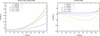 |
Fig. D.1 Radii of massive stars (five masses as given in key) as a function of age in units of main sequence lifetime; right panel: results by standard SSE; left panel: results from our upgraded SSE. |
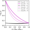 |
Fig. E.1 Figure showing the family of functions for the original treatment foriginal(q, y) and the family of functions with our updated treatment fupdated(q, y) for three distinct values of y ∈ (−1, −2, −3) against the mass ratio q of the MS star collision parnters. |
Appendix F Hardware settings
The simulations are executed on the Raven high performance computing system at the Max Planck Computing and Data Facility (MPCDF)3. Here, we use from one to three full GPU computing node for the simulation, which gives the optimal performance and most cost-effective use of the computing resources. Each GPU computing node is equipped 4 Nvidia A100 GPUs (4 × 40 GB HBM2 memory per node and NVLink). Furthermore, each node has one CPU hosts, which is an Intel Xeon IceLake Platinum 8360Y with 72 CPU cores. The RAM is 512 GB per node or 256 GB of RAM depending on the node you get assigned to via the slurm system. For a detailed account including benchmarking concerning the optimal performance of the Nbody6++GPU code on hybrid, GPU-accelerated supercomputers, please refer to the recent review by Spurzem & Kamlah (2023) and sources therein. Even using this state-of-the-art high performance computing (HPC) infrastructure, the simulation take up to 2 months of real time to reach a star cluster age of 5 Myr. Tests and developments on machines such as juwels-booster in Germany4, Lumi in Finland and Leonardo in Italy were done. We expect more data from these infrastructures soon.
MOCCA simulations for this work were performed on the ’chuck’ computer cluster at the Nicolaus Copernicus Astronomical Center of the Polish Academy of Sciences (CAMK PAN) in Warsaw, Poland. Taking the same initial model generated by Mcluster for the direct N-body simulation, we used MOCCA to evolve the system up to 7 Myr within approximately 10 hours on a single CPU core. The high computational efficiency of the MOCCA code proved extremely valuable for iterative testing and debugging, particularly in identifying and resolving the stellar radius evolution issue discussed in Appendix B.
All Tables
Initial conditions of our star cluster model and the most important features related to the stellar evolution of all the stars.
All Figures
|
Fig. 1 Initial mass of the cluster as a function of the half-mass radius. The color bar represents the number of particles. The dashed black line represents the relaxation time, and the dotted black line corresponds to the collision time when both are equal to a time evolution (i.e., age) of τ = 10 Gyr, which we considered as an upper limit for the typical evolutionary times of the clusters. The symbols indicate different simulations: N-body (squares), Monte Carlo (circles), hybrid N-body (diamonds), and this work (star). |
| In the text | |
|
Fig. 2 Average mass in each Lagrangian shell 〈M〉Lagr[M⊙] (top) and the Lagrangian radii RLagr [pc] (bottom), both normalized by the cluster mass at the beginning of the simulation. We show the N-body and MOCCA results for the Lagrangian radii. The two plot show the shell representing 1%, 10%, 30%, 50%, 70%, and 90%. The differences between the Lagrangian radii in the N-body and MOCCA simulations arise from how escaping stars are treated. In the N -body simulations, stars with positive energy are not immediately removed from the system; instead, they remain until they cross a boundary set at ten times the half-mass radius. These stars are still included in the calculation of Lagrangian radii, which affects the results compared to MOCCA. |
| In the text | |
|
Fig. 3 Cumulative mass of escapees (top panel) and cumulative number of collisions (bottom panel). The total number of collisions is represented by a solid black line (N-body) and solid magenta line (MOCCA), while collisions involving the VMS are shown with a dot-dashed purple line (N-body) and solid cyan line (MOCCA). The binaries involving the VMS are shown with a dotted red line, and hyperbolic collisions with the VMS are shown by a dashed blue line. |
| In the text | |
|
Fig. 4 Top panels: mass of each escaping star. Bottom panels: mass of the secondary star before it collides with the VMS for hyperbolic and binary collisions. The color bar represents the density distribution of the stars. |
| In the text | |
|
Fig. 5 Histograms showing the contribution of colliding stars to VMS formation, divided into binary, hyperbolic, and total collisions. The mass ranges are < 0.1 M⊙, 0.1-1 M⊙, 1-10 M⊙, 10-100 M⊙, and > 100 M⊙. Results are shown for the N-body simulation (left column) and the MOCCA simulation (right column). The top panel displays the number of collisions, and the bottom panel shows the cumulative mass contributed by these collisions. |
| In the text | |
|
Fig. 6 Temporal evolution of the position of the VMS relative to the star cluster density center, ξVMS,IMBH, and the speed of the VMS relative to the star cluster density center, νVMS,IMBH. |
| In the text | |
|
Fig. 7 Temporal evolution of a hard binary system during between 1.68 and 1.80 Myr. This binary has the primary star as the VMS, with a mass of 28 891 M⊙ and a secondary star with a mass of 75 M⊙. This interaction lasts approximately 0.1 Myr. The top panel shows the semimajor axis, while the bottom panel shows the eccentricity. |
| In the text | |
|
Fig. 8 Evolution of the VMS (and IMBH thereafter) over time. Top panel: mass of the VMS/IMBH, MVMS,IMBH [M⊙]. Middle panel: stellar radius of the VMS/IMBH, RVMS,IMBH [R⊙] (logarithmic scale). Bottom panel: effective age of the VMS during its main-sequence phase, AVMS,IMBH [Myr]. |
| In the text | |
|
Fig. D.1 Radii of massive stars (five masses as given in key) as a function of age in units of main sequence lifetime; right panel: results by standard SSE; left panel: results from our upgraded SSE. |
| In the text | |
|
Fig. E.1 Figure showing the family of functions for the original treatment foriginal(q, y) and the family of functions with our updated treatment fupdated(q, y) for three distinct values of y ∈ (−1, −2, −3) against the mass ratio q of the MS star collision parnters. |
| In the text | |
Current usage metrics show cumulative count of Article Views (full-text article views including HTML views, PDF and ePub downloads, according to the available data) and Abstracts Views on Vision4Press platform.
Data correspond to usage on the plateform after 2015. The current usage metrics is available 48-96 hours after online publication and is updated daily on week days.
Initial download of the metrics may take a while.