| Issue |
A&A
Volume 704, December 2025
|
|
|---|---|---|
| Article Number | A106 | |
| Number of page(s) | 13 | |
| Section | Planets, planetary systems, and small bodies | |
| DOI | https://doi.org/10.1051/0004-6361/202555555 | |
| Published online | 08 December 2025 | |
Scattering of light by cosmic dust: Parameterized Mueller matrix
Department of Physics, University of Helsinki,
Gustaf Hällströmin katu 2,
PO Box 64,
00014
Helsinki,
Finland
★ Corresponding author: This email address is being protected from spambots. You need JavaScript enabled to view it.
Received:
16
May
2025
Accepted:
15
October
2025
Abstract
Context. The scattering matrix averaged for a particle ensemble is a 4 × 4 Mueller matrix that describes, as a function of the scattering angle, θ, the relation between polarized light incident on and scattered by the ensemble. An empirical system is provided for the angular dependencies of the matrix elements for the commonly occurring case of arbitrarily shaped particles and their mirror particles that are both oriented randomly. The resulting Mueller matrix, F, is of a block-diagonal form and is given by six nonzero functions F11, F12 = F21, F22, F33, F34 = -F43, and F44.
Aims. It is our goal to show that the complex angular dependencies of the Mueller matrix can be parameterized with the help of analytical basis functions. The empirical system strives to remove obstacles arising from, for example, measured or computed scattering matrices violating the strict symmetry relations among the elements. The system further allows for efficient application of the scattering matrices.
Methods. The empirical system is based on insights from the physics of light scattering. The angular dependencies are taken to be functions of q = sin 1/2θ, a functional form frequently present in scattering problems. With the proposed modeling, common matrices can be represented by using a minimum of 28 free parameters in total; that is, less than five parameters as per the matrix element. Markov chain Monte Carlo schemes are provided for the estimation of the parameters and their uncertainties.
Results. Examples of experimentally measured and theoretical scattering matrices are analyzed with the help of the empirical system. The Mueller matrix elements are typically matched, in a relative sense, with a root-mean-square value on the order of 1%. The example Mueller matrices provide a range of angular patterns, acting as a credible test bench for the system.
Conclusions. The system with related numerical methods is successful in capturing the angular dependencies of the scattering matrix elements. The system allows for applications in both forward and inverse scattering problems concerning cosmic dust particles, with prospects for applications in scattering problems at large.
Key words: polarization / radiative transfer / scattering / comets: general / minor planets, asteroids: general / planets and satellites: general
© The Authors 2025
 Open Access article, published by EDP Sciences, under the terms of the Creative Commons Attribution License (https://creativecommons.org/licenses/by/4.0), which permits unrestricted use, distribution, and reproduction in any medium, provided the original work is properly cited.
This article is published in open access under the Subscribe to Open model. This email address is being protected from spambots. You need JavaScript enabled to view it. to support open access publication.
1 Introduction
The Stokes parameters of light incident on and scattered by particles are interrelated by a 4 × 4 Mueller matrix, the scattering matrix (van de Hulst 1957; Bohren & Huffman 1998). The scattering matrix contains complete information about the scattering process; in other words, how polarized incident light is transformed into polarized scattered light. In the scattering phase matrix here termed F, a normalization is introduced by separating the integrated scattering cross section for unpolarized incident light from the scattering matrix and normalizing the F11-element, the scattering phase function, to 4π in the integration over the solid angle.
A commonly encountered scattering phase matrix is blockdiagonal, resulting from averaging over a particle ensemble. Natural particle ensembles can typically be assumed to consist of particles and their mirror particles, both oriented randomly in space. In such a case, the nonzero elements of the matrix are the diagonal elements F11, F22, F33, and F44 and the off-diagonal elements F12 = F21 and F34 = -F43.
The scattering matrices play a crucial role in scattering problems related to cosmic dust. We develop an empirical parameterization for the block-diagonal scattering phase matrix based on physics and practical aspects, striving toward a user-friendly formulation for inverse light-scattering problems and other applications. Before that, we offer a concise overview of related studies.
Baes et al. (2022) provide a recent review of empirical models for the scattering phase function. They further develop a two-term ultraspherical phase function, pointing out that the new phase function improves the scattering modeling, in particular, outside the spectral range of visible light.
The Henyey-Greenstein scattering phase function is by far the most commonly used empirical phase function (Henyey & Greenstein 1941). It allows for analytical manipulations and is parameterized by the asymmetry parameter, the average for the cosine of the scattering angle, characterizing the scattering into forward- and backward-directed hemispheres. Introducing two Henyey-Greenstein terms is a popular approach as it allows for realistic increases in the phase function toward both the forward-and backward-scattering directions.
Isotropic, Legendre polynomial, and Rayleigh phase functions are among the early choices for the phase function (e.g., Chandrasekhar 1960). These are, however, quite specific and have restrictions insofar as their application to wavelength-scale particle scattering is concerned.
Pollack & Cuzzi (1980) introduced a semiempirical scattering phase function for wavelength-scale particles based on three components. Mie theory is used for particles smaller than a given threshold in terms of the size parameter x = ka, where k = 2π/λ is the wave number for the wavelength, λ, and a describes the radial size. Above the threshold, the phase function is based on three components. The first component, diffraction, is modeled by using physical optics. The second component, external reflection, derives from geometric optics. The third component involves a single-parameter exponential expression. Pollack & Cuzzi (1980) obtained good matches for the semiempirical phase function and measured or computed phase functions. Bowell et al. (1989) extended the modeling with additional exponential terms and came up with an average scattering phase function for applications in multiple scattering by planetary regoliths.
Braak et al. (2001) devised an empirical phase matrix with the Henyey-Greenstein phase function and a scalable Rayleighlike degree of linear polarization. In order to allow for mathematically correct modeling of phase matrices, Domke (1974) introduced a series presentation in generalized spherical functions (see also de Haan et al. 1987). Due to the large number of coefficients in the series presentations and the nonlocal character of the basis functions, the generalized spherical functions are an inconvenient choice for the variation of matrix elements in, for example, inverse light-scattering problems.
Cubic splines have turned out to be highly useful in the presentation of Mie scattering phase matrix elements for arbitrary scattering angles, when the exact element values are available for a uniform set of scattering angles (e.g., angular resolution of a degree; Muinonen 2004). Furthermore, splines are an excellent choice for smoothening elements, either measured or computed, that may include random errors (e.g., Muñoz et al. 2012; Muinonen et al. 1996). For splines applied to wavelengthscale particles, some 15 nodes adaptively selected across the scattering-angle range can be sufficient for an accurate presentation. Consequently, using splines would result in coefficients on the order of 102 for presenting the six matrix elements. For controlled variation in the elements, splines are not optimal due to the large number of parameters, difficulties in enforcing symmetry relations (Hovenier & van der Mee 1983; Hovenier & van der Mee 2000), and local changes producing unwanted undulations in the angular patterns.
An earlier phenomenological scattering phase matrix has been developed for radiative transfer and coherent backscattering applications to atmosphereless planetary-system objects by Muinonen & Videen (2012). In that work, the phase matrix was modeled as a sum of two pure Mueller matrices with a double Henyey-Greenstein phase function. While the phenomenological matrix has been successfully used in the polarimetric modeling of icy satellites (Ejeta et al. 2013; Kiselev et al. 2022, 2024), it suffers from a number of shortcomings. First, the double Henyey-Greenstein phase function does not allow for satisfactory presentations of phase functions measured or computed for small particles. Second, there are limitations for the angular characteristics of matrix element ratios, making the modeling of measured and computed ratios challenging.
In Section 2, we introduce the ensemble-averaged scattering phase matrix together with the symmetry relations among its elements. We introduce the parameters and basis functions for the novel empirical phase matrix and describe the parameter constraints arising from the symmetry relations. The section further presents a number of additional descriptors for the matrix elements. In Section 3, we summarize parameter optimization methods and present Markov chain Monte Carlo (MCMC) methods for the evaluation of plausible parameter ranges. Section 4 focuses on the modeling of experimental and theoretical scattering phase matrices by using the empirical system. The set of examples serves to illustrate how the free parameters affect the shapes of the matrix elements. In Section 5, we close the study with conclusions and future prospects.
2 Scattering matrix
2.1 Ensemble-averaged scattering phase matrix
Consider a particle ensemble that includes equal numbers of nonspherical particles and their mirror particles, both in random orientation. The average 4 × 4 scattering phase matrix, F = F(θ), of the ensemble relates the Stokes parameters of incident light, Ii = (Ii, Qi, Ui, Vi)T, to those of scattered light, Is = (Is, Qs, Us, Vs)T (θ is the scattering angle, a spherical polar angle with θ = 0 refering to the forward-scattering direction; Bohren & Huffman 1998),
 (1)
(1)
Here σs and r denote the scattering cross section for unpolarized incident light and the distance between the scatterer and the observer, respectively. The scattering phase matrix takes the block-diagonal form (Hovenier & van der Mee 2000)
 (2)
(2)
where we have the common normalization of
 (3)
(3)
We assessed the functions b1, a2, a3, b2, and a4 relative to a1 and, for convenience, defined
 (4)
(4)
The scattering phase matrix is subject to symmetry relations (Hovenier & van der Mee 2000). For arbitrary scattering angles,
![Mathematical equation: \begin{eqnarray} |a_{j{\rm r}}(\theta) | &\leq& 1, \;\;\; j=2,3,4, \nonumber\\ |b_{j{\rm r}}(\theta) | &\leq& 1, \;\;\; j=1,2, \nonumber\\ ~ [a_{3{\rm r}}(\theta) +a_{4{\rm r}}(\theta)]^2+4b_{2{\rm r}}^2(\theta) &\leq& [1 +a_{2{\rm r}}(\theta) ]^2 - 4b_{1{\rm r}}^2(\theta), \nonumber\\ |a_{3{\rm r}}(\theta) -a_{4{\rm r}}(\theta) | &\leq& 1 - a_{2{\rm r}}(\theta), \nonumber\\ |a_{2{\rm r}}(\theta) -b_{1{\rm r}}(\theta) | &\leq& 1 - b_{1{\rm r}}(\theta), \nonumber\\ |a_{2{\rm r}}(\theta) +b_{1{\rm r}}(\theta) | &\leq& 1 + b_{1{\rm r}}(\theta). \label{eqfsym} \end{eqnarray}](/articles/aa/full_html/2025/12/aa55555-25/aa55555-25-eq6.png) (5)
(5)
In the forward and backward directions,
 (6)
(6)
2.2 Empirical system
We introduced a parameterized scattering phase matrix that captures the overall angular characteristics of typical ensemble-averaged experimental and theoretical phase matrix elements. The matrix elements are described as follows for arbitrary scattering angles, θ, through the dependence of  :
:
![Mathematical equation: \begin{eqnarray} a_1 &=& \frac{D_{1}}{1+d_{1}q^{\delta_1}} + \frac{R_{1}}{1+r_{1}p^{\rho_1}} + S_1\exp(-s_1 p^{\sigma_1}), \nonumber\\ a_{j{\rm r}} &=& D_{j} p^{\delta_j} + R_{j} q^{\rho_j} + S_j\exp(-s_j p^{\sigma_j}), \;\;\; j=2,3,4, \nonumber\\ b_{j{\rm r}} &=& A_j p^{\beta_j} q^{\gamma_j} + H_{j} p^{\beta_j} \left[1 - \exp\left(- h_j q^{\eta_j}\right)\right] \nonumber\\ && +\, K_{j} q^{\gamma_j} \left[1 - \exp\left(- k_j p^{\kappa_j}\right)\right] , \;\;\; j=1,2, \label{eqpemp} \end{eqnarray}](/articles/aa/full_html/2025/12/aa55555-25/aa55555-25-eq9.png) (7)
(7)
where
 (8)
(8)
We note that the system parameters are relevant only in the regime of parameter phase space, where the symmetry relations of Eqs. (5) and (6) are fulfilled. The parameterization is nonlinear and it is possible to arrive at equally satisfactory representations of the scattering matrix elements in different parts of the parameter space.
In the most general form in Eq. (7), there are 48 parameters describing six functions of θ. For a1 as a rule of thumb, the parameter triplets D1, d1, δ1 and R1, r1, ρ1 characterize the angular dependencies in the forward-scattering (“D” for “drive”) and backward-scattering (“R” for “reverse”) regimes, whereas the triplet S, s1, σ1 describes backscattering characteristics for narrow to moderate angular ranges (“S” for “surge”). For ajr(j = 2, 3,4), the doublet Dj, δj and the quintet Rj, ρj, Sj, Sj, σj refer to the forward- and backward-scattering regimes, respectively. For bjr (j = 1,2), the triplet Aj, βj, γj refers to the overall angular characteristics, whereas the triplets H1, h1, η1 and K1, k1, κ1 refer to the forward- and backward-scattering regimes, respectively. Taking into account the condition of a1 in Eq. (3) and the two conditions for ajr (j = 2, 3,4) in Eq. (6), the number of free parameters reduces to 44. Furthermore, the triplets Sj, Sj, σj (j = 1,2, 3,4) and the parameters ηj and κj (j = 1,2) do not need to be always utilized, so the number of free parameters reduces to 28, which implies, on average, fewer than five free parameters for each of the six functions.
The a1 model in Eq. (7) emerges from the Q-factor algebra (Sorensen et al. 2017) in the forward-scattering regime (see also van de Hulst 1957). Sorensen et al. (2017) show that the scattering phase functions, a1, of varying small particle ensembles show a linear dependence on the logarithmic scale in the forward-scattering regime, when the phase functions are expressed as a function of  . In Eq. (7), a regularization of the linear dependence is introduced with the help of a rational function to remove the singularity in the forward-scattering direction. Furthermore, the wave number, k, does not enter the a1 model (thus,
  ). It is clear that alternative basis functions can be introduced, when the particular forward-scattering characteristics are of interest (for example, the Fraunhofer diffraction pattern). The a1 model includes an analogous dependency in the backward-scattering regime, suggested by the forward- and backward-propagating internal electromagnetic waves within small scattering particles, giving rise to similarities in forward- and backward-scattered waves (Muinonen et al. 2011). Finally, in order to account for a backward-scattering surge often detected for small particles (e.g., Lumme & Rahola 1998; Muñoz et al. 2012), an additional exponential-trigonometric term is introduced.
As was described above for ajr (j = 2,3,4), there are formally seven parameters for each (the Dj, δj and Rj, ρj doublets and the Sj, Sj, σj triplets), amounting to 21 parameters in total. The symmetry relations in Eq. (6) introduce conditions that reduce the number of free parameters to 18:
 (9)
(9)
With the help of Eqs. (7) and (6), we express D3, R3, and R4 with the help of D2, R2, S2, s2, S3, s3, and S4:
 (10)
(10)
For the matrix element ratios b1r and b2r, there are nine free parameters for each. In addition to the argumentation above, the model is motivated by the trigonometric and linear-exponential models for polarimetric phase curves of atmosphereless Solar System objects (Lumme & Muinonen 1993; Penttilä et al. 2005; Muinonen et al. 2009). There are, however, differences: the present system allows for vanishing first derivatives in the backward- and forward-scattering directions and is thus applicable to scattering matrices of small particles.
2.3 Additional descriptors
As the exponents of the empirical system in Eq. (7) relate to the physics of scattering, they serve as useful descriptors of the angular dependencies. However, due to the complex parameter interplay, additional descriptors are called for to characterize the dependencies.
For the scattering phase function a1, the norm is by definition N11 = 1 and the asymmetry parameter g11 describes the balance between scattering into forward and backward hemispheres (to distinguish between the descriptors, a numerical subscript of the matrix element in Eq. (2) was used),
 (11)
(11)
The predicted values in the forward and backward directions are of interest, as is the minimum value, a1↓ and the corresponding scattering angle, θ11↓:
 (12)
(12)
Note that a1(0) and a1(π) are independent of the exponents δ1, ρ1, and σ1.
For the off-diagonal element b1, N12 and g12 (Muinonen 2004), analogous to the parameters for a1, describe the polarizing efficiency and asymmetry, respectively,
 (13)
(13)
Natural descriptors of −b1r are the minimum and maximum degrees of polarization, −b1r↓ and −b1r↑, as well as the corresponding scattering angles, θ12↓ and θ12↑, together with the inversion angle, θ12i,
 (14)
(14)
If there are two negative branches present, one near backward scattering and another near forward scattering, they can both be characterized similarly. For the off-diagonal element b2r, the characterization is analogous.
For a2r, a3r, and a4r, the values at forward- and backwardscattering directions are of interest,
 (15)
(15)
The minimum and maximum values of these elements (not repeating the values in the forward- and backward-scattering directions) and the corresponding scattering angles can be used as descriptors,
 (16)
(16)
For the elements a3r and a4r, the inversion angles θ33i and θ44i (when relevant) can be utilized,
 (17)
(17)
3 Numerical methods
Least-squares optimization of the parameters was carried out by using the Nelder-Mead downhill simplex method (Press et al. 1992) and parameter uncertainties were evaluated with MCMC methods (cf., O’Hagan & Forster 2004). Note that, since the system is empirical in its nature, the parameters and their uncertainties must be treated with caution rather than related to the first principles of physics. Throughout the numerical methods, the sets of parameters to be incorporated in the analyses can be selected by the user.
Given the analytical expressions for the matrix elements, simple Matlab routines have been developed for the initial estimation of the parameters, complemented with a systematic mapping of the parameter space by using a Fortran implementation. While mapping the parameter space, symmetry relations are monitored and enforced. Least-squares optimization is then initialized in the proximity of the plausible solution, substantially improving the prospects for success in detecting the global and realistic extremum.
We followed Bayesian inference in defining a posteriori probability density function (p.d.f.), pp(P), for the free parameters (unknowns), P (e.g., Muinonen et al. 2020), by assuming a constant a priori p.d.f. We utilized the Metropolis-Hastings algorithm with a symmetric Gaussian proposal p.d.f., pt(P; P″) (the subscript “t” stands for transition). Here pt is a product of uncorrelated monovariate Gaussian densities. The MCMC algorithm proceeds by the computation of the ratio ar:
 (18)
(18)
Here Pj and P″ denote the current and proposed parameters in a Markov chain, respectively. The proposed parameters, P″, are accepted or rejected with the help of a uniform random deviate, y ∈ [0,1]:
 (19)
(19)
The proposed parameters are thus accepted with the probability of min(1, ar). After a number of transitions in the burn-in phase, the Markov chain, in the case of success, converges on sampling the target p.d.f. pp.
In our practical implementation, the MCMC part can first be carried out separately for all the matrix elements, completing the analysis for a1 that is independent of the remaining matrix element ratios. Thereafter, the final MCMC simulation concerns simultaneously the five element ratios a2r, a3r, a4r, b1r, and b2r. The root-mean-square (rms) values, σrms, of the least-squares fits are computed from
![Mathematical equation: \sigma_{\rm rms} &=& \sqrt{ \frac{1}{N_{\rm obs}} \sum_{j=1}^{N_{\rm obs}} \left[ m_j - M(\theta_j,{\bf P})\right]^2},](/articles/aa/full_html/2025/12/aa55555-25/aa55555-25-eq24.png) (20)
(20)
where Nobs denotes the number of observations, mj and M(θj, P) stand for the observed and computed element values for a1r, a2r, a3r, a4r, −b1r, and b2r, respectively, and θj denote the scattering angles. Here the element a1r is logarithmic and corresponds to
 (21)
(21)
Furthermore, the restricted nature of the empirical model in Eq. (7) results in systematic differences between the observed scattering phase matrix elements and their model counterparts. We mitigated the systematics by introducing a so-called slip factor in the uncertainty model; that is, by increasing the formal standard deviation computed from the rms value of the leastsquares fit with a factor based on reducing the correlation from an expected high initial value to a targeted low final value. The procedure corresponds to adding a sufficient amount of fictitious white noise into the uncertainty model to mitigate the systematics. In what follows, we set the initial value of correlation to 0.9 and targeted the final value to be 0.1.
4 Results and discussion
We present example modeling results for polarimetric measurements obtained from the updated Granada-Amsterdam Light Scattering Database (Muñoz et al. 2025). Because measurements near the exact forward- and backward-scattering directions are typically subject to larger uncertainties, we limited the use of the measured data to the angular range between 10° and 173°. Furthermore, only those scattering angles for which all six Mueller matrix elements are available were retained. The exception was the numerical scattering simulations for water ice particles, in which case the full angular range of the data was used, as all matrix elements are available at all angles. The ice particle example further serves to illustrate that there are limitations in the use of the empirical scattering matrix system.
Across all samples, the empirical system demonstrates a consistent performance, reproducing the measured scattering behavior while adhering to symmetry constraints. Residual correlations were mitigated by introducing a sufficient amount of fictitious white noise during the data processing. For conciseness, a posteriori p.d.f.s of the parameters were characterized by the means and the standard deviations from the MCMC solutions and by the uncertainty envelopes for a number of example scattering matrices. The model parameters and their uncertainties expressed as standard deviations are summarized in Tables A.1 and A.2.
In order to supplement the model parameters, we incorporated key additional descriptors for the elements a1 and −b1r, which offer an enhanced physical insight into the scattering behavior. For the scattering phase function, a1, the asymmetry parameter, g11, is detailed. Regarding the degree of linear polarization, −b1r, we provide the polarizing efficiency, N12, the associated asymmetry parameter, g12, and the maximum and minimum polarization degrees, −b1r↑ and −b1r↓. The remaining supplementary descriptors, which include extrema and inversion angles for a2r, a3r, a4r, and b2r, are compiled into Tables A.3 and A.4 as mean values derived from the MCMC analyses, accompanied by their respective standard deviations.
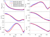 |
Fig. 1 Scattering phase matrix elements for the Allende meteorite sample: measurements (circles; Granada-Amsterdam Light Scattering Database) and modeling (solid line; present empirical system) at the wavelengths of 441.6 nm (blue) and 632.8 nm (red). |
4.1 Allende meteorite
To demonstrate the capability of the parameterization, we begin with the measurement of a crushed sample of the Allende meteorite (Muñoz et al. 2000). The sample in the Granada-Amsterdam Light Scattering Database has a refractive index of 1.65 + i0.001, an effective particle size of reff = 0.8 μm, and an effective variance of veff = 3.3, indicating that the sample consists of small particles with a wide size distribution. The effect of the size distribution can be seen in Fig. 1, where only a slight wavelength dependency is shown, as well as in Tables A.1 through A.4. The Allende sample is a carbonaceous chondrite and shows strong forward scattering with high a1(0) and gn, but a low polarizing efficiency, with shallow −b1r extrema and low N12. Figure 1 shows the measured data (36 data points in both the 441.6 nm and 632.8 nm datasets) alongside the modeling results. The rms values based on Eq. (20) for the elements lg a1, −b1r, a2r, a3r, b2r, and a4r are shown in Table A.1. In general, the modeling captures the features of the measured data well. The rms values are better than 1.2% for the 441.6 nm dataset and better than 2.0% for the 632.8 nm dataset. However, in the case of −b1r, the analysis reveals slight differences at small scattering angles. It remains unclear whether these differences arise from limitations in the system or from uncertainties in the measurements themselves. Near the backward scattering direction, the linear polarization does not decrease as much as in the measured data. These differences most likely result from the small number of measurement data near the forward- and backward-scattering directions, causing the other directions to have excessive weight in the modeling.
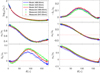 |
Fig. 2 As in Fig. 1, but for the lunar surface analog (JSC-1A) at wavelengths of 488 nm (blue), 520 nm (green), and 647 nm (red). |
4.2 Lunar analog
According to the rms values presented in Table A.2 for the lunar analog datasets (Escobar-Cerezo et al. 2018), modeling across all three wavelengths (488, 520, and 647 nm, each comprising 36 data points) generally yields a good agreement with the measurements. Nevertheless, the data corresponding to 488.0 nm pose certain challenges, exhibiting subtle differences in the angular dependence of the matrix elements (Fig. 2), which are likely to be attributable to noise within the measured data. The rms values are 0.41-4.6%, 0.49-2.7%, and 0.46-1.4% for the 488 nm, 520 nm, and 647 nm datasets, respectively (Table A.2). The database provides a refractive index for the sample akin to that of Allende, estimated to be 1.65 + i0.003, with reff = 10.50 1 μm and veff = 1.69, indicating a sample of large particles with a comparatively wide size distribution.
Overall, the findings demonstrate a satisfactory agreement for additional descriptors, including the minimum and maximum degrees of polarization, as well as the inversion angle. Symmetry constraints require the a4r element to display a pronounced peak near the backward scattering direction, where experimental data are unavailable. Further investigation is warranted to ascertain whether this phenomenon arises as an artifact from the fitting process or constitutes an intrinsic characteristic of polarization. We consider it to be more likely the latter, as analogous surges result in theoretical studies. The lunar analog sample demonstrates stable and well-developed polarimetric behavior across the wavelengths examined. Its −b1r↓ and −b1r↓ values consistently exhibit robustness, and its a2r↓ and a4r↓ extrema remain relatively constant, implying scattering behavior insensitive to wavelength, which is likely to result from self-similarity due to a broad distribution of scatterer sizes.
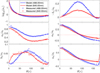 |
Fig. 3 As in Fig. 1, but for the Martian surface analog (MMS-2L) at the wavelengths of 488 nm (blue) and 640 nm (red). |
4.3 Martian analog
For the Martian analog, we present results at the wavelengths of 488 and 640 nm (Martikainen et al. 2024, 2025) with 32 and 35 points in the respective datasets. This red-brown-colored sample has reeff = 16.2 μm, a small effective variance, veff = 0.12, and a refractive index of 1.5 + i0.0011 at 488 nm and 1.5 + i0.0035 at 640 nm. It offers an illustrative case of wavelength-dependent scattering behavior (Fig. 3).
The empirical system reproduces the measured scattering matrix elements overall with rms values of 0.45-3.4% for the 488 nm dataset and 0.39-2.6% for the 640 nm dataset (Table A.2). The 488 nm data exhibit slight deviations in the off-diagonal elements, −b1r and b2r, where the former shows a less pronounced negative branch compared to the measurements. Additionally, the a4r element deviates slightly from the measured values, which could be attributed to noise in the measurements for b2r.
Similar to the lunar analog, the Martian analog displays a significant surge in the a4r element near the backward scattering direction, where measurement data are lacking. The sample displays a contrasting wavelength dependence. At 640 nm compared to 488 nm, MMS-2L shows a marked decrease in forwardscattering intensity and polarization amplitude, as is indicated by the decreasing trends in g11, − b1r↑, and the overall spread of Mueller matrix descriptors. The spectral sensitivity of its scattering properties distinguishes MMS-2L from the more stable silicate-rich materials in the dataset.
4.4 Feldspar
Feldspar, measured at 441.6 nm and 632.8 nm by Volten et al. (2001), represents the second case of wavelength-dependent measurements with 36 points in both datasets. The sample has reff = 1.0 μm and veff = 1.0, and the refractive index is estimated to have a real part of 1.5 to 1.6 and an imaginary part between 10−5 and 10−3. As is shown in Fig. 4, the modeling closely follows the measured data for both wavelengths. The rms values are small, at 0.24-1.0% for the 441.6 nm dataset and 0.28-0.88% for the 632.8 nm dataset (Table A.1). The differences in linear polarization, especially the amplitude and location of the negative polarization extremum, are well captured by the empirical system. However, at 632.8 nm there is a mild underestimation of the degree of linear polarization (−b1r) near the backward scattering direction.
Feldspar exhibits strong forward scattering and a high polarizing efficiency, particularly at longer wavelengths. In Fig. 4, the effect of the particle size distribution is clearly visible, when the wavelength changes from 441.6 nm to 632.8 nm. This spectral change is not limited to amplitude: the spread between a2r↓ and a2r↑ is consistent with small particle size and narrow size distribution.
4.5 Hematite and rutile
Hematite and rutile are samples featuring high refractive indices, small effective particle sizes, and narrow size distributions. For hematite, the size distribution is described by reff = 0.4 μm and veff = 0.6 and the complex refractive index is 3.0 + i[0.01-0.1]. The rutile sample has reff = 0.13 μm and veff = 0.5, with the real part of the refractive index 2.73 and the imaginary part near-zero. Both datasets correspond to a wavelength of 632.8 nm and include 36 data points (Shkuratov et al. 2004; Muñoz et al. 2006).
The polarization features are irregular for both samples, with a multilobed degree of linear polarization, −b1r(θ). These features likely stem from the high refractive indices, optical anisotropy, or fine internal structures. They show pronounced matrix elements that are characterized by more complex angular dependencies, particularly in the off-diagonal matrix elements. The empirical system successfully reproduces these features (see Table A.1). For hematite, the rms values range across 0.161.2% and, for rutile, across 0.23-2.6%. Additionally, we present 10 000 MCMC results, visualized as uncertainty envelopes (hematite and rutile in Figs. 5 and 6, respectively). The results indicate that the model captures the dominant trends well and produces reliable outcomes. However, the lack of measurements near the backward-scattering and forward-scattering directions introduces uncertainties in these regions.
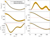 |
Fig. 5 Scattering phase matrix elements for the hematite sample: measurements (circles; Granada-Amsterdam Light Scattering Database) and modeling (solid line; empirical system). The uncertainty envelope (orange) depicts the minimum and maximum values from 10 000 MCMC sample solutions. |
4.6 Water ice
The scattering phase matrix for water ice, as presented in Muinonen & Markkanen (2023) with 181 points in the dataset, represents the most challenging scenario for the empirical system, containing more features than the measured data available. The fitting results, in conjunction with lg aι, a3r, and a4r, nevertheless demonstrate a reasonable fit, with rms values of 2.2-4.9% (Table A.2).
Conversely, −b1r provides an adequate fit solely for scattering angles surpassing 50 degrees, while tending to average out prominent features below this threshold. The rms value is still excellent, at 1.1%.
In contrast, for b2r, there are difficulties in reaching values as high as those anticipated by theoretical data near the backwardscattering direction, yet an otherwise satisfactory fit is achieved with an rms value of 2.2%. Meanwhile, a2r corresponds well to the data near both forward and backward scattering, whereas the system falls short at intermediate scattering angles, with the resulting rms value as high as 7.6%.
Simulated water ice stands out with the most extreme forward scattering (highest g11), a broad negative polarization structure, and a distinct backward-scattering peak in a4r. Water ice shows unique behavior when compared with other samples, reinforcing its unique role as a reference for high-albedo surfaces such as those found on icy moons of giant planets or Kuiper Belt objects.
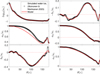 |
Fig. 7 Scattering phase matrix elements computed and ensemble-averaged for Gaussian-random-sphere particles composed of water ice (circles) and as described by the empirical system (solid line). |
4.7 Comparative analysis with empirical descriptors
Figures 8 and 9 present a descriptor-based comparative analysis of scattering behavior across an example set of materials, derived by using the empirical scattering matrix system. The figures visualize physically meaningful quantities computed from the modeled matrix elements, such as the asymmetry parameter, gu, linear polarization extrema, −b1r↓ and −b1r↑, and various angular characteristics of a2r, a3r, and a4r.
Figure 8 reveals a correlation between δ1 and g11 (top left). Across the sample set, higher values of δ1, which correspond to narrower forward-scattering lobes in the model phase function, generally lead to larger g11, consistent with enhanced forward-directed scattering. This trend is particularly evident for weakly absorbing silicate and icy materials such as feldspar and water ice. However, the correlation weakens for samples such as hematite and rutile, whereas, while δ1 and g11 are not directly linked in all cases, their joint behavior captures important distinctions in scattering.
The parameters δ1 and ρ1 (Fig. 8, top right) control the angular confinement of the forward- and backward-scattering lobes, respectively, in the model phase function a1. The lack of a clear correlation between these descriptors indicates that the scattering mechanisms responsible for forward and backward scattering are largely different across the sample set. This separation highlights the flexibility of the empirical system in accommodating complex scattering behaviors present in planetary regolith analogs.
A secondary trend appears between the polarizing efficiency, N12 - that is, the integrated strength of linear polarization across all angles - and the polarization asymmetry parameter, g12 (Fig. 8, bottom left). This indicates that materials with higher overall linear polarization tend to exhibit polarization curves that are directionally biased. This relationship suggests that the angular structure and strength of linear polarization are connected. It is interesting that both N12 and g12 span positive and negative values. Based on N12, this refers to the scatterers being net positively or negatively polarizing. For the former cases, g12 is systematically positive, referring to the tendency of stronger positive polarization in the forward-scattering hemisphere and stronger negative polarization in the backward-scattering hemisphere. In contrast, for the latter cases, g12 shows both negative (ice) and positive values (rutile). For ice, the negative value derives from strong positive polarization in the backward-scattering hemisphere and negative polarization in the forward-scattering hemisphere (Fig. 7). In comparison, for rutile, the angular ranges of positive and negative polarization are exchanged (Fig. 6). Notice that N12 and g12 relate to −b 1 rather than −b1r.
In Fig. 8 (bottom right), many samples with deep negative polarization minima (−b1r↓) span a broad range of positive polarization maxima (−b1r↑), indicating that, while both features often co-occur, their amplitudes can vary independently. This spread likely testifies to the combined influence of sample properties. The clustering in values of −b1r↓ however, should be studied further in future work as it may suggest shared physical mechanisms underpinning both polarization extrema, with certain materials maximizing the angular polarization contrast more effectively than others.
Figure 9 extends the analysis to the angular behavior of the remaining matrix element ratios. It begins by comparing the minimum and maximum values of a2r for those samples where both extrema are present, illustrating the angular modulation of linearly polarized incident light by the samples (top left). In Fig. 9 (top right), a3r(π) is shown versus a3r(0), illustrating the expected antisymmetric behavior of the element, consistent with theoretical symmetry relations for scattering by randomly oriented particles (Hovenier & van der Mee 2000). Finally (Fig. 9, bottom left and right), relationships in a4r↓ vs. a4r(0) and the extrema b2r↕ of |b2r| with the corresponding angle, θ34r↕, suggest that strong backward-scattering features in polarization are consistent across silicate-rich materials.
A comparative look at multiple wavelengths reveals two cases with distinct spectral trends. Feldspar (441.6 nm vs. 632.8 nm) shows increased a1(0) and −b1r↑ at longer wavelengths, indicating enhanced forward scattering and polarization. It also shows a broader spread between minimum and maximum values for the red wavelength (632.8 nm) compared to the blue one (441.6 nm), indicating that the angular modulation of linear polarization retention becomes more pronounced with wavelength. This suggests that, in addition to amplitude scaling, feldspar’s scattering matrix undergoes subtle wavelengthdependent reshaping. In contrast, the Martian analog MMS-2L displays a suppression of both forward scattering and polarization at 640 nm compared to 488 nm. The shift is evident in both descriptor values and matrix element behavior pointing to decreased absorption at longer wavelengths. The spectral sensitivity of MMS-2L’s matrix elements further distinguishes it from silicate-rich samples.
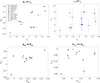 |
Fig. 8 Additional descriptors derived from the parameterized scattering phase matrix elements a1 and b1 for selected materials: the asymmetry parameter, g11, versus the forward-scattering exponent, δ1 (top left), the backward-scattering exponent, ρ1, versus δ1 (top right), the polarization asymmetry parameter, g12, versus the polarizing efficiency, N12 (bottom left), and the minimum degree of linear polarization, -b1r↓, versus the corresponding maximum, -b1r↑ (bottom right). |
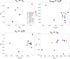 |
Fig. 9 Angular characteristics of selected scattering phase matrix element ratios for the sample materials: the minimum versus maximum values of a2r (top left), a3r in the backward-scattering direction versus the same element ratio in the forward-scattering direction (top right), the minimum value of a4r versus the same ratio in the forward-scattering direction (bottom left), and the extreme value b2r↕ in the absolute sense versus the corresponding scattering angle, θ34↕ (bottom right). |
5 Conclusions
We have provided a parameterized Mueller matrix for light scattering by cosmic dust particles. The resulting scattering phase matrix is analytical, user-friendly, and gives accurate representations of experimental and theoretical phase matrices. The empirical matrix comes with initialization, least-squares optimization, and MCMC schemes for the estimation of the free parameters. Hence, we have shown that it is possible to parameterize scattering phase matrices and simultaneously fulfil the symmetry relations among the matrix elements. We have illustrated the concept by applying the framework to 12 different cases of scattering phase matrices.
There are significant future prospects for the empirical scattering matrix system. First, we aim to analyze all the scattering matrices in the Granada-Amsterdam Light Scattering Database (Muñoz et al. 2012) and unveil possible trends in the parameters. Second, we expect to utilize the empirical system in inverse multiple scattering problems concerning the disk-integrated photometric and polarimetric phase curves of atmosphereless Solar System objects. Third, it may be possible to further improve the basis functions with the help of an artificial intelligence approach.
Acknowledgements
Research supported by the Research Council of Finland through grants nos. 336546 and 359893.
References
- Baes, M., Camps, P., & Kapoor, A. U. 2022, A&A, 659, A149 [NASA ADS] [CrossRef] [EDP Sciences] [Google Scholar]
- Bohren, C., & Huffman, D.R. 1998, Absorption and Scattering of Light by Small Particles (Wiley Science Paperback Series) [Google Scholar]
- Bowell, E., Hapke, B., Domingue, D., et al. 1989, in Asteroids II, eds. R. P. Binzel, T. Gehrels, & M. S. Matthews (University of Arizona Press), 524 [Google Scholar]
- Braak, C., de Haan, J., van der Mee, C., Hovenier, J., & Travis, L. 2001, J. Quant. Spec. Radiat. Transf., 69, 585 [Google Scholar]
- Chandrasekhar, S. 1960, Radiative Transfer (Dover) [Google Scholar]
- de Haan, J. F., Bosma, P. B., & Hovenier, J. W. 1987, A&A, 183, 371 [Google Scholar]
- Domke, H. 1974, Ap&SS, 29, 379 [Google Scholar]
- Ejeta, C., Muinonen, K., Boehnhardt, H., et al. 2013, A&A, 554, A117 [NASA ADS] [CrossRef] [EDP Sciences] [Google Scholar]
- Escobar-Cerezo, J., Muñoz, O., Moreno, F., et al. 2018, ApJS, 235, 19 [NASA ADS] [CrossRef] [Google Scholar]
- Henyey, L. G., & Greenstein, J. L. 1941, ApJ, 93, 70 [Google Scholar]
- Hovenier, J. W., & van der Mee, C. V. M. 1983, A&A, 128, 1 [NASA ADS] [Google Scholar]
- Hovenier, J., & van der Mee, C. 2000, Basic Relationships for Matrices Describing Scattering by Small Particles, eds. M. I. Mishchenko, J. W. Hovenier, & L. D. Travis (Academic Press), 61 [Google Scholar]
- Kiselev, N., Rosenbush, V., Muinonen, K., et al. 2022, Planet. Sci. J., 3, 134 [Google Scholar]
- Kiselev, N., Rosenbush, V., Leppälä, A., et al. 2024, Planet. Sci. J., 5, 10 [Google Scholar]
- Lumme, K., & Muinonen, K. 1993, in IAU Symposium 160, Asteroids, Comets, Meteors 1993, Book of Abstracts, Belgirate, Italy, 194 [Google Scholar]
- Lumme, K., & Rahola, J. 1998, J. Quant. Spec. Radiat. Transf., 60, 439 [Google Scholar]
- Martikainen, J., Muñoz, O., Martín, J. C. G., et al. 2024, ApJS, 273, 28 [Google Scholar]
- Martikainen, J., Muñoz, O., Gómez Martín, J. C., et al. 2025, MNRAS, 537, 1489 [Google Scholar]
- Muinonen, K. 2004, Waves Random Media, 14, 365 [Google Scholar]
- Muinonen, K., & Videen, G. 2012, J. Quant. Spec. Radiat. Transf., 113, 2385 [Google Scholar]
- Muinonen, K., & Markkanen, J. 2023, in Light, Plasmonics and Particles, eds. M. P. Mengüç, & M. Francoeur, Nanophotonics (Elsevier), 149 [Google Scholar]
- Muinonen, K., Nousiainen, T., Fast, P., Lumme, K., & Peltoniemi, J. 1996, J. Quant. Spec. Radiat. Transf., 55, 577 [Google Scholar]
- Muinonen, K., Penttilä, A., Cellino, A., et al. 2009, Meteorit. Planet. Sci., 44, 1937 [NASA ADS] [CrossRef] [Google Scholar]
- Muinonen, K., Tyynelä, J., Zubko, E., et al. 2011, J. Quant. Spec. Radiat. Transf., 112, 2193 [Google Scholar]
- Muinonen, K., Torppa, J., Wang, X.-B., Cellino, A., & Penttilä, A. 2020, A&A, 642, A138 [NASA ADS] [CrossRef] [EDP Sciences] [Google Scholar]
- Muñoz, O., Volten, H., De Haan, J., Vassen, W., & Hovenier, J. 2000, A&A, 360, 777 [Google Scholar]
- Muñoz, O., Volten, H., Hovenier, J., et al. 2006, A&A, 446, 525 [NASA ADS] [CrossRef] [EDP Sciences] [Google Scholar]
- Muñoz, O., Moreno, F., Guirado, D., et al. 2012, J. Quant. Spec. Radiat. Transf., 113, 565 [CrossRef] [Google Scholar]
- Muñoz, O., Frattin, E., Martikainen, J., et al. 2025, J. Quant. Spec. Radiat. Transf., 331, 109252 [Google Scholar]
- O’Hagan, A., & Forster, J. J. 2004, Kendall’s Advanced Theory of Statistics: Bayesian Inference, 2nd edn., 2B (Arnold) [Google Scholar]
- Penttilä, A., Lumme, K., Hadamcik, E., & Levasseur-Regourd, A.-C. 2005, A&A, 432, 1081 [NASA ADS] [CrossRef] [EDP Sciences] [Google Scholar]
- Pollack, J. B., & Cuzzi, J. N. 1980, Scattering by Non-Spherical Particles of Size Comparable to a Wavelength: A New Semi-Empirical Theory, eds. D. W. Schuerman (Boston, MA: Springer US), 113 [Google Scholar]
- Pollack, J. B., & Cuzzi, J. N. 1980, J. Atmos. Sci., 37, 868 [NASA ADS] [CrossRef] [Google Scholar]
- Press, W. H., Teukolsky, S. A., Vetterling, W. T., & Flannery, B. P. 1992, Numerical Recipes in C, (2nd edn.): The Art of Scientific Computing (USA: Cambridge University Press) [Google Scholar]
- Shkuratov, Y., Ovcharenko, A., Zubko, E., et al. 2004, J. Quant. Spec. Radiat. Transf., 88, 267 [NASA ADS] [CrossRef] [Google Scholar]
- Sorensen, C. M., Heinson, Y. W., Heinson, W. R., Maughan, J. B., & Chakrabarti, A. 2017, Atmosphere, 8 [Google Scholar]
- van de Hulst, H. C. 1957, Light Scattering by Small Particles (Dover) [Google Scholar]
- Volten, H., Muñoz, O., Rol, E., et al. 2001, J. Geophys. Res. Atmos., 106, 17375 [Google Scholar]
Appendix A Auxiliary tables
Scattering matrix parameters for feldspar, Allende, hematite, and rutile.
Scattering matrix parameters for lunar analog, Martian analog, and water ice particles.
Additional descriptors for feldspar, Allende, hematite, and rutile.
Additional descriptors for lunar analog, Martian analog, and water ice particles.
All Tables
Scattering matrix parameters for lunar analog, Martian analog, and water ice particles.
Additional descriptors for lunar analog, Martian analog, and water ice particles.
All Figures
|
Fig. 1 Scattering phase matrix elements for the Allende meteorite sample: measurements (circles; Granada-Amsterdam Light Scattering Database) and modeling (solid line; present empirical system) at the wavelengths of 441.6 nm (blue) and 632.8 nm (red). |
| In the text | |
|
Fig. 2 As in Fig. 1, but for the lunar surface analog (JSC-1A) at wavelengths of 488 nm (blue), 520 nm (green), and 647 nm (red). |
| In the text | |
|
Fig. 3 As in Fig. 1, but for the Martian surface analog (MMS-2L) at the wavelengths of 488 nm (blue) and 640 nm (red). |
| In the text | |
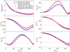 |
Fig. 4 As in Fig. 1, but for feldspar at the wavelengths of 441.6 nm (blue) and 632.8 nm (red). |
| In the text | |
|
Fig. 5 Scattering phase matrix elements for the hematite sample: measurements (circles; Granada-Amsterdam Light Scattering Database) and modeling (solid line; empirical system). The uncertainty envelope (orange) depicts the minimum and maximum values from 10 000 MCMC sample solutions. |
| In the text | |
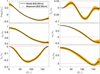 |
Fig. 6 As in Fig. 5, but for rutile. |
| In the text | |
|
Fig. 7 Scattering phase matrix elements computed and ensemble-averaged for Gaussian-random-sphere particles composed of water ice (circles) and as described by the empirical system (solid line). |
| In the text | |
|
Fig. 8 Additional descriptors derived from the parameterized scattering phase matrix elements a1 and b1 for selected materials: the asymmetry parameter, g11, versus the forward-scattering exponent, δ1 (top left), the backward-scattering exponent, ρ1, versus δ1 (top right), the polarization asymmetry parameter, g12, versus the polarizing efficiency, N12 (bottom left), and the minimum degree of linear polarization, -b1r↓, versus the corresponding maximum, -b1r↑ (bottom right). |
| In the text | |
|
Fig. 9 Angular characteristics of selected scattering phase matrix element ratios for the sample materials: the minimum versus maximum values of a2r (top left), a3r in the backward-scattering direction versus the same element ratio in the forward-scattering direction (top right), the minimum value of a4r versus the same ratio in the forward-scattering direction (bottom left), and the extreme value b2r↕ in the absolute sense versus the corresponding scattering angle, θ34↕ (bottom right). |
| In the text | |
Current usage metrics show cumulative count of Article Views (full-text article views including HTML views, PDF and ePub downloads, according to the available data) and Abstracts Views on Vision4Press platform.
Data correspond to usage on the plateform after 2015. The current usage metrics is available 48-96 hours after online publication and is updated daily on week days.
Initial download of the metrics may take a while.