| Issue |
A&A
Volume 704, December 2025
|
|
|---|---|---|
| Article Number | A166 | |
| Number of page(s) | 11 | |
| Section | Extragalactic astronomy | |
| DOI | https://doi.org/10.1051/0004-6361/202555673 | |
| Published online | 09 December 2025 | |
An extremely high-velocity outflow in SMSS J2157-3602, the most luminous quasar in the first 1.3 Gyr
1
INAF – Istituto di Astrofisica Spaziale e Fisica cosmica Milano, Via Alfonso Corti 12, 20133 Milano, Italy
2
Physical Sciences Division, School of STEM, University of Washington Bothell, Bothell, WA 98011, USA
3
Institute for Astronomy, University of Edinburgh, Royal Observatory, Blackford Hill, Edinburgh EH9 3HJ, UK
4
INAF, Osservatorio Astronomico di Roma, Via Frascati 33, I– 00078 Monte Porzio Catone, Italy
5
School of Physics, HH Wills Physics Laboratory, University of Bristol, Tyndall Avenue, Bristol BS8 1TL, UK
6
Department of Physics and Astronomy, York University, 4700 Keele Street, Toronto, ON M3J 1P3, Canada
7
Dipartimento di Fisica, Sapienza Universtià di Roma, Piazzale Aldo Moro 5, 00185, Rome
8
INAF – Osservatorio Astronomico di Trieste, Via Tiepolo 11 34143 Trieste, Italy
9
IFPU – Institute for Fundamental Physics of the Universe, Via Beirut 2, 34014 Trieste, Italy
10
INAF – Osservatorio di Astrofisica e Scienza dello Spazio di Bologna, Via Gobetti, 93/3, 40129 Bologna, Italy
11
School of General Education, Shinshu University, 3-1-1 Asahi, Matsumoto, Nagano 390-8621, Japan
12
Research School of Astronomy and Astrophysics, Australian National University, Cotter Road, Weston Creek ACT 2611, Australia
13
Centre for Gravitational Astrophysics (CGA), Australian National University, Building 38 Science Road, Acton ACT 2601, Australia
14
Dipartimento di Fisica ed Astronomia (DIFA), Università di Bologna, Via Gobetti, 93/2, 40129 Bologna, Italy
⋆ Corresponding author: This email address is being protected from spambots. You need JavaScript enabled to view it.
Received:
26
May
2025
Accepted:
8
September
2025
Abstract
We report the discovery of an extremely high-velocity outflow (EHVO) in the most luminous QSO (LBol ∼ 2.29 × 1048 erg/s), named SMSS J2157-3602, at z = 4.692. Combined XSHOOTER and NIRES observations reveal that the EHVO reaches a maximum velocity of vmax ∼ 0.13c and persists over rest-frame timescales of a few months up to one year. SMSS J2157-3602 also exhibits one of the highest balnicity index values discovered for an EHVO so far. In addition, the blueshifted CIV emission traces a high-velocity (vCIV50 ∼ 4660 km/s) outflow from the broad-line region (BLR). Thanks to an XMM-Newton observation, we were also able to reveal the X-ray weak nature of this QSO, which likely prevents the overionization of the innermost disk atmosphere and facilitates the efficient launch of the detected EHVO and BLR winds. The extraordinary luminosity of SMSS J2157-3602 and the extreme velocity of the EHVO make it a unique laboratory for testing active galactic nucleus (AGN) driven feedback under extreme conditions. Current uncertainties on the outflow’s location and column density strengthen the case for a dedicated follow-up, which will be essential to assess the full feedback potential of this remarkable quasar.
Key words: galaxies: active / quasars: absorption lines / quasars: supermassive black holes / quasars: individual: SMSS J2157-3602
© The Authors 2025
 Open Access article, published by EDP Sciences, under the terms of the Creative Commons Attribution License (https://creativecommons.org/licenses/by/4.0), which permits unrestricted use, distribution, and reproduction in any medium, provided the original work is properly cited.
This article is published in open access under the Subscribe to Open model. This email address is being protected from spambots. You need JavaScript enabled to view it. to support open access publication.
1. Introduction
Outflows originating from the inner regions around supermassive black holes (SMBHs) are detected in a substantial fraction of QSOs (up to ∼50%) as blueshifted absorption lines in their UV and X-ray spectra (e.g., Crenshaw et al. 2003; Blustin et al. 2005; Misawa et al. 2007; Bischetti et al. 2022; Tombesi et al. 2010; Matzeu et al. 2023). The most dramatic nuclear outflows are represented by the ultra-fast (up to 0.2–0.5c) outflows (UFOs) discovered in X-rays through highly blueshifted absorption features of He- and H-like Fe at E > 7 keV, which originate at tens up to hundreds gravitational radii from the SMBH (Tombesi et al. 2012). Their high velocities imply significant kinetic powers (ĖK,ufo), making up as much as 10–20% of the QSO bolometric luminosity, as  (King & Pounds 2015). Therefore, UFOs might be crucial in the study of feedback mechanisms, as they represent potentially the most energetic outflows due to their higher velocities, leading to the injection of a significant amount of energy into the surrounding ISM sufficient to influence the evolution of the host galaxy.
Absorption lines in rest-frame UV spectra are usually classified into three categories: broad absorption lines (BALs) with a full width at half maximum of FWHM ≥ 2000 km s−1, narrow absorption lines (NALs) with FWHM ≤ 500 km s−1, and mini-BALs (500 ≤ FWHM ≤ 2000 km s−1). BALs have typically been identified within the velocity range of 5000 to 25 000 km s−1 (Weymann et al. 1991). However, such features can reach velocities of ∼50 000–60 000 km s−1 or more, prompting the introduction of a new term: extremely high velocity outflows (EHVOs; Rodríguez Hidalgo et al. 2011). Hereafter, the term “EHVO” denotes BAL outflows with velocities of v > 25 000 km s−1.
Over the past decade, the number of sources detected with EHVOs has increased, expanding from individual quasars (e.g., Rodríguez Hidalgo et al. 2011; Rogerson et al. 2016; Bruni et al. 2019) to hundreds of QSOs (Rodríguez Hidalgo et al. 2020, hereafter RH2020, and Rodríguez Hidalgo in prep). Indeed, RH2020 recently conducted a pioneering survey of EHVOs in the general SDSS QSO population, analyzing 6743 QSOs and detecting 40 QSOs with EHVOs, which were found to be more prevalent at higher luminosities. These EHVOs were identified in the UV spectrum primarily through CIV and NV absorption at speeds between 10% and 20% of the speed of light (i.e., similar to X-ray UFOs). Specifically, the detection is based on the fact that SiIV absorption always displays a corresponding CIV absorption outflowing at similar speeds, with no cases reported so far in the literature of quasar outflows where SiIV absorption is present without corresponding CIV. Therefore, an absorption feature between Lyα and SiIV without corresponding CIV can be ascribed to a CIV EHVO.
Here, we report the discovery of an EHVO in the most luminous QSO known to date in the first 1.3 Gyr after the Big Bang at z = 4.692: SMSS J215728.21-360215.1 (hereafter SMSS J2157; Wolf et al. 2018).
Its discovery was enabled by the photometric and astrometric data from SkyMapper Southern Sky Survey (SMSS), Wide-field Infrared Survey Explorer (WISE), and Gaia, with an estimated bolometric luminosity of 1.6 × 1048 erg/s, inferred from the monochromatic luminosity at 3000 Å (Onken et al. 2020). An anisotropy-corrected bolometric luminosity based on the spectral energy distribution (SED) is presented in Lai et al. (2023) and the SED-based estimate derived in this work is discussed in Sect. 3.2. SMSS J2157 was not detected in any large radio survey (National Radio Astronomy Observatory Very Large Array Sky Survey (NVSS) f1.4GHz < 2.5 mJy (Condon et al. 1998), Sydney University Molonglo Sky Survey (SUMSS) f843MHz < 5.0 mJy (Bock et al. 1999)); therefore, it is classified as radio-quiet QSO (Wolf et al. 2018).
SMSS J2157 hosts a SMBH with an estimated MgII-based BH mass of MBH ∼ 3.4 × 10¹⁰ M⊙, placing it among the largest black holes known to date, and an Eddington ratio λEdd ∼ 0.4 (Onken et al. 2020; see also Lai et al. (2023) for accretion disc-based BH mass estimate and corresponding Eddington ratio). Recent observations using the XSHOOTER instrument (Vernet et al. 2011) at the Very Large Telescope (VLT) and the Near-Infrared Echellette Spectrometer (NIRES) instrument (Wilson et al. 2004) at Keck Observatory have suggested the presence of a potential EHVO in SMSS J2157 spectra. In this paper, we analyze the absorption feature observed in the rest-wavelength range 1350–1400 Å, confirming its EHVO nature with a maximum velocity of ∼42 350 km/s. In Sect. 2, we present the spectroscopic observations and the reconstruction of the UV spectrum. In Sect. 3, we characterize the EHVO detected in SMSS J2157. Sect. 3.2 provides results from spectral and photometric analysis and Sect. 3.3 present the total column density derivation. In Sect. 4, we describe the XMM-Newton observations, including the data reduction and analysis and we discuss the X-ray properties of SMSS J2157. In Sect. 5, we analyze the kinematics and energetics of the EHVO in SMSS J2157, highlighting the associated large uncertainties. Finally, in Sect. 6, we summarize our findings. In this work, we assume that Ωm = 0.27, ΩΛ = 0.73, and H0 = 70 km s1 Mpc−1 (Komatsu et al. 2011).
2. Observations and data reduction
2.1. Spectral datasets
We analyzed spectroscopic observations obtained with the XSHOOTER instrument (Vernet et al. 2011) at the Very Large Telescope (VLT). Details of the observations are listed in Table 1. Specifically, we used XSHOOTER data (Program ID: 0103.B-0949(A)) with SMSS J2157 observed in 2019 June 03 and 2019 July 08. The data reduction of the XSHOOTER data was performed using the XSHOOTER pipeline version within the ESO-Reflex environment (version 2.11.5; Modigliani et al. 2010). Science spectra for each arm were individually reduced, adopting the nodding mode setting in the pipeline. For flux calibration, standard stars were observed and reduced using the same calibration data as the science frames. The telluric line correction was carried out with molecfit (Smette et al. 2015). Finally, we applied the barycentric velocity correction for each spectrum. For simplicity, we refer to these data as XSHOO-1 and XSHOO-2 spectrum, respectively. We also included the dataset presented by Onken et al. (2020), which combines Keck/NIRES spectra from June 2018 with VLT/XSHOOTER data from October 2019. Hereafter, we refer to this dataset as NIRES-XSHOO. A detailed description of the spectroscopic observations and data reduction procedures can be found in Onken et al. (2020).
Journal of observations.
We rescaled XSHOO-1, XSHOO-2 and NIRES-XSHOO spectra to the J-band VHS Data Release 6 (JVega = 15.65 ± 0.01, Wolf et al. 2018) and SkyMapper z-band magnitudes (zAB = 17.11 ± 0.02, Wolf et al. 2018). No significant variability was observed between the June and July observations of XSHOO-1 and XSHOO-2 spectra, we then averaged them and rebinned the final coadded 1D spectrum to match the NIRES-XSHOO spectrum bin size (50 km s−1). Since no further variability was detected between this final coadded 1D spectrum and the NIRES-XSHOO spectrum, both spectra were also averaged. Additionally, public light curve data from the NASA/ATLAS survey in the o-band (orange filter, ∼560–820 nm) show only minor variability over a four-year period (2017–2021), supporting our findings. The final spectrum is shown in Fig. 1.
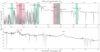 |
Fig. 1. Final coadded spectrum of SMSS J2157, with the CIV, NV, and Lyα EHVO highlighted in light red. The blended NALs systems are indicated in aquamarine. The AlIII+CIII] and MgII emission lines are also marked. Regions affected by telluric absorption are marked in light grey. |
2.2. Reconstruction of the rest-frame UV spectrum
As shown in Fig. 1, several low-velocity (v ≤ 25 000 km/s; shades of cyan) BAL features are present, with matching velocity ranges blueward of CIV, SiIV, NV, and OVI. The absence of an absorption feature blueward of MgII indicates that SMSS J2157 is a high-ionization BAL quasar, in contrast to low-ionization BAL quasars, which also show absorption from low-ionization species such as MgII.
However, as described in Sect. 2.3 and shown in Fig. A.1, although the CIV trough satisfies the classical observational definition of a BAL (e.g., Weymann et al. 1991), our line profile modeling reveals that it results from the superposition of multiple narrow absorption components (FWHM < 500 km s−1), indicating that this is a blended-NAL system.
These absorption features are superimposed on their respective emission lines. The trough blueward of SiIV is significantly broader in velocity than the absorption features blueward of CIV, suggesting that part of this feature may be attributed to an EHVO of the CIV ion (RH2020). This absorption is likely accompanied by an EHVO of NV and possibly Lyα at a similar velocity, which fall within the Lyα forest. To properly account for the complex blend of SiIV emission line, where both the SiIV blended NALs and the CIV EHVO are present, as well as the corresponding NV and Lyα EHVO in the Lyα forest region, we adopted a two-step approach.
We first derived the best-fit model of the continuum, using a custom Python-based code (e.g., Vietri et al. 2022) to simultaneously fit the continuum with a power law and the principal emission lines: Lyα, NVλ1240, SiVλ1398, OIVλ1402, CIVλ1549, HeIIλ1640, OIII]λ1663, AlIIIλ1857, SiIIIλ1887, and CIII]λ1909, using Gaussian components while masking all narrow and broad absorption lines. The model fitting was performed in the spectral region at 1210–2000 Å, to prevent the intervening absorption on the blue side of Lyα from affecting the fit. Therefore, we extrapolated the continuum to the blue side of the Lyα from the best-fit model. We then used a reconstruction model to provide a best estimate of the emission lines and avoid underestimating the strength of the absorption features. The reconstruction was generated via the scheme developed for Rankine et al. (2020), which is based on an independent component analysis (ICA; Højen-Sørensen et al. 2002; Opper & Winther 2005; Allen et al. 2013) of SDSS quasars. The ICA components were linearly combined to reproduce the intrinsic emission, which is particularly useful in cases where much of the emission has been absorbed. The ICA components were generated from and for reconstructing low-S/N SDSS spectra; however, the data used here are of higher resolution (c.f. R ∼ 2000 for SDSS, R ∼ 5400, 8900, 5600 for UVB, VIS, and NIR arms of XSHOOTER, respectively) and higher S/N. To reconstruct the spectrum, we first re-binned the spectrum onto the Δlog λ = 0.0001 wavelength grid of SDSS (using SPECTRES; Carnall 2017). The reconstruction scheme can then be applied to the spectrum to produce a reconstruction covering 1275–3000 Å. Part of the routine masks bad pixels and narrow absorption features that are N-σ below the continuum level (where σ is the noise array). Since the routine was fine-tuned for SDSS-level S/N and resolution, we repeated the spectral fitting with a grid of N values: N = 1/8, 1/6, 1/4, 1/2, 1, 2, 3, and we also degraded the S/N of the spectrum by multiplying the noise array by a factor of 8, 6, 4, 2, and 1. The reconstructed spectra created with all combinations of these parameters are presented in Fig. 2 alongside the median reconstruction. On first inspection the reconstructions appear to differ significantly at the CIV and SiIV emission; however, the majority of the individual reconstructions are similar to the median reconstruction and of them ended up inferring stronger emission lines. The median reconstruction was then adopted to normalize the spectrum between 1275–3000 Å, along with the best-fit model continuum blueward of the Lyα line (as shown in Fig. 3).
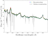 |
Fig. 2. Median spectral reconstruction (black) created from the reconstructions with different parameters used in the spectral fitting. The original spectrum is plotted in grey. The regions affected by telluric absorption are marked as light grey color. |
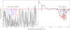 |
Fig. 3. Normalized, coadded spectrum of SMSS J2157, overlaid with the best-fit model (red curve) for the EHVO features of the CIV doublet (three blue-red pairs of dashed Gaussian components for modeling 1548,1550 Å lines respectively), NV doublet (three blue-red pairs of dotted Gaussian curves for modeling 1238,1242 Å lines respectively), Lyα (three blue dash-dotted Gaussian curves), and SiIV doublet blended NALs (seven green-purple pairs of dotted Gaussian components for modeling 1393,1402 Å lines, respectively). The spectrum was normalized to the reconstructed model at λ > 1275 Å and to the extrapolated continuum λ < 1275 Å. |
From the median reconstruction, we performed a direct line integration to derive the CIV emission line equivalent width, obtaining EW(CIV) ∼ 17 ± 2 Å, placing it marginally within the weak emission line regime as defined by Chen et al. (2024). We also calculated the 50th percentile velocity,  km/s1, indicating a strong outflow originating from the broad-line region (BLR). These values of EW and velocity shift of the CIV emission line are consistent with the properties found for the EHVO sample analyzed in Rodríguez Hidalgo & Rankine (2022). EHVOs are characterized by low EW(CIV) and significant blueshifts in the CIV emission line, exhibiting values that are more extreme than the average observed in both non-BAL and BAL QSOs (Rodríguez Hidalgo & Rankine 2022).
2.3. Blended SiIV NAL removal from CIV EHVO region
As mentioned above, the CIV EHVO falls in the same location as the SiIV blended NAL at lower velocity. To avoid overestimating the amount of CIV EHVO, we proceeded to fit and remove the SiIV from this region in an iterative process.
We assumed that the normalized observed flux at a given velocity I(v) is described by:
![Mathematical equation: $$ \begin{aligned} I(v) = [1 - C_f] + C_f e^{-\tau (v)} .\end{aligned} $$](/articles/aa/full_html/2025/12/aa55673-25/aa55673-25-eq4.gif) (1)
(1)
The parameter Cf is the coverage fraction (0 < Cf < 1; Hamann & Ferland 1999) and τ(v) is the optical depth, which we assumed to follow a Gaussian profile characterized by the central optical depth (τ0), centroid velocity (μ), and Doppler parameter (b).
Initially, we plotted the SiIV doublet2, visually adjusting the component widths and centroid velocities to match the observed profiles. We then fit the corresponding CIV blended NAL region (see Fig. A.1 in Appendix A), maintaining the same widths and centroid velocities derived from the SiIV region, allowing only the optical depths to vary. The initial fit indicated the need for additional, weaker NAL components. These were iteratively added until a satisfactory fit was achieved. We observed the CIV blended NAL system to be saturated at about 2% of the continuum flux level, which is a sign of Cf lower than 1. The best-fit solution yielded a constant Cf = 0.98 value for this region. The final component widths and centroid velocities were then adopted to model the SiIV NAL doublets as described in the next section.
3. Results from spectral and photometric analysis
3.1. Analysis of the EHVO
To model the CIV EHVO absorption, which is blended with lower-velocity SiIV NALs, we performed a simultaneous fit of both components. For the SiIV blended NALs, we kept the Doppler parameters and centroid velocities fixed, as described in Sect. 2.3, and left the optical depths free to vary.
We modeled the CIV EHVO doublet with a Gaussian profile for each component, as described in Sect. 2.3. Up to three doublets were used to model the CIV EHVO absorption. The central optical depth, centroid velocity, and Doppler parameter of each component were left free to vary. The covering fraction, Cf, was systematically explored by evaluating values between 0.1 and 1. For each fixed Cf, we performed 100 fits with randomized initial parameters for all Gaussian components. The global best-fit solution was obtained for Cf = 1, which minimizes both χ2 and the Bayesian information criterion (BIC), as shown in Fig. 3. We therefore adopted the Cf = 1 solution as our fiducial best-fit model. Solutions with very low Cf (≈0.1–0.41), corresponding to a quasi-saturated regime, are strongly disfavored by the fit statistics (ΔBIC ≫ 10); whereas solutions with Cf ≥ 0.44 are statistically equivalent (ΔBIC < 10) and cannot be formally excluded. This range of acceptable Cf values allowed us to estimate a conservative range for the hydrogen column density, NH, by considering NH derived for Cfmin = 0.44 and Cfmax = 1 (see Sect. 3.3).
We then used the CIV EHVO best-fit model as a template to fit the NV doublet and Lyα EHVO troughs, which were blended with the Lyα forest. In this fit, only the optical depths were allowed to vary, while the Doppler parameters and centroid velocities were kept fixed. Since the NV and Lyα absorption features fall within the Lyα forest, we treated our measurements in this region as the upper limits. Figure 3 also shows the best-fit model for the NV doublets and Lyα EHVO.
From the best-fit model of the CIV EHVO, we measured the Balnicity index (BI; Weymann et al. 1991) to characterize the CIV EHVO absorption by adopting 25 000 and 60 000 km/s as minimum and maximum velocity integration limits,
![Mathematical equation: $$ \begin{aligned} \mathrm{BI} = - \int _{60{\,}000}^{25{\,}000} \left[1 - \frac{f({v})}{0.9} \right] C \, dv ,\end{aligned} $$](/articles/aa/full_html/2025/12/aa55673-25/aa55673-25-eq5.gif) (2)
(2)
where we adopted as f(v) the CIV EHVO best-fit model as a function of the velocity, v, and C is a constant set to unity if the spectrum is at least 10 percent below the continuum model for velocity widths of at least 1000 km s−1 and zero otherwise.
We calculated the CIV BI km s−1, placing it in the top ∼20% of the BI distribution for BAL quasars at lower redshifts (Gibson et al. 2009) and among the largest values discovered so far for EHVOs with velocities exceeding 35 000 km s−1 (see RH2020). We derived a minimum velocity for the CIV EHVO of vmin ∼ 31 170 km s−1 and a maximum velocity of vmax ∼ 42 350 km s−1. The velocities are given relative to the longer-wavelength component of the CIV doublet, assuming the relativistic Doppler effect. We also derived an upper limit for BI of the NV doublet and Lyα EHVO, namely, BI
 km s−1 and BI
 km s−1, respectively.
3.2. Spectral energy distribution
We model the SED spanning from the X-ray to MIR-infrared wavelengths. We used publicly available photometric data in the YJKs bands from the VISTA Hemisphere Survey (McMahon et al. 2013) in the H band from the Two Micron All-Sky Survey (Skrutskie et al. 2006) and W1-W4 bands from the Wide-field Infrared Survey Explorer (Wright et al. 2010). Comprehensive details about the photometry can be found in the discovery paper (Wolf et al. 2018).
Additionally, we used observations obtained with the Rapid Eye Mount (REM) telescope at the La Silla Observatory in November 7, 2019 (PI: V. Testa), using the ROS2 visible photometric channel. A series of nine images were acquired with the SDSS-griz filters, and each exposure lasted 240 s. All the images were processed using the jitter script from the eclipse package (Devillard 1997). This script aligns and stacks series of images to create an average frame for each sequence, while also performing a sky subtraction. The magnitudes measured for the optical griz filters have been calibrated against several field stars selected from the APASS catalogue (DR9, Henden et al. 2016) by performing differential photometry using an aperture of 8 pixels (corresponding to ∼4.6 arcsec). Table 2 lists the REM AB magnitudes, corrected for the galactic extinction using values reported in Schlafly & Finkbeiner (2011). We also used X-ray data point obtained with XMM-Newton and presented in Sect. 4.
SMSS J2157 optical magnitudes obtained with REM.
We performed SED fitting for the luminosity points at λ ≥ 1216 Å. To avoid having the fit driven by points with very low uncertainties, we added an error of 0.1 mag in quadrature for each data point’s uncertainty (e.g., Boquien et al. 2019). To model the SED, we used three templates of optically selected Type-1 QSOs, distinguished by increasing infrared-to-optical flux ratios, namely, BQSO1, QSO1, and TQSO1, taken from the SWIRE template library Polletta et al. (2007). Given the extreme luminosities of the source, the host emission can be considered negligible (e.g., Shen et al. 2011). For each template, we maximized the likelihood using emcee (Foreman-Mackey et al. 2019):
 (3)
(3)
where yi represents the photometric data points at the i-th filter, and fi denotes the flux obtained by convolving the SED template with the i-th filter. Then, K is the normalization factor of the template, and Aλ = Kλ(E(B − V)) is the dust-reddening law from Prevot et al. (1984), accounting for possible contributions from dust extinction. For both K and E(B − V), we assumed flat, non-negative priors. Since the BQSO1 template provided the best fit, yielding the highest likelihood value, we reported the quantities computed with it. We obtained a color excess E(B − V) = 0.07 ± 0.005, where the uncertainties are quoted as the 16th and 84th percentiles. The best-fit de-reddened (purple curve) and reddened (pink curve) SEDs are shown in Fig. 4.
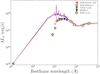 |
Fig. 4. Best-fit de-reddened and reddened SEDs with 1σ errors for SMSS J2157 (purple and pink lines, respectively), as derived in Sect. 3.2. The 1 keV luminosity is shown as a left-pointing coral red triangle; REM/ROS2 g, r, i, z data are represented by orange circles; Y, J, and Ks points from VISTA are shown as down-pointing green triangles; the H point from 2MASS is represented by a down-pointing blue triangle; and golden yellow squares represent the W1-W4 WISE channels. The uncertainties of data points are shown but are smaller than the symbol size. |
The bolometric luminosity was computed by integrating the best-fit SED from 1 μm to 1 keV, resulting in Log(LBol/erg s−1) = 48.36. Hereafter, we adopted this value of LBol in our analysis. Since the employed templates only extended up to 900 Å, we extrapolated the EUV region of the SED using the double power-law recipe from Lusso et al. (2010) and Saccheo et al. (2023). Specifically, this is λLλ ∝ λ0.8 down to λ = 500 Å, plus a power law with a free-to-vary index to connect the 1 keV luminosity with the 500 Å one.
3.3. Ionic column densities and photoionization solution
Using the Gaussian profiles of the CIV and NV doublets and Lyα corresponding to the minimum and maximum acceptable covering fractions (Cfmin = 0.44 and Cfmax = 1), as derived in Sect. 3.1, we calculated the ionic column density Nion (Arav et al. 2001) as follows
 (4)
(4)
where λ is the laboratory wavelength and f is the oscillator strength corresponding to a specific ion. We used the numerical code Cloudy (version C23, Chatzikos et al. 2023) to compute the fraction of ionic species by varying the ionization parameter, U, assuming the gas is in photoionisation equilibrium and solar abundances (Lodders 2003), along with the broadband SED of SMSS J2157, described in Sect. 3.2 (see Fig. 4).
We found Nion = 3.3 × 1015 cm−2 (1.3 × 1016 cm−2), Nion = 9.3 × 1015 cm−2 (3.7 × 1016 cm−2), and Nion = 3.6 × 1015 cm−2 (1.5 × 1016 cm−2) for CIV, NV, and Lyα ions, respectively, for Cfmax (Cfmin).
Using the fraction of ionic species and ionic column densities calculated from Eq. (4), we derived the total hydrogen column density, NH, as a function of U, for both Cfmin and Cfmax. In Fig. 5, we show the NH curves as a function of U, along with the possible solutions which are highlighted in bold lines, considering NH curves of Lyα and NV as upper limits. From this analysis, we found NH = [4.9 × 10¹⁹–3.5 × 10²¹] cm−2 for Cfmax and NH = [2 × 10²⁰–1.4 × 10²²] cm−2 for Cfmin. For a conservative estimate, we adopted the median values, NHCfmax = 2.8 × 1020 cm−2 and NHCfmin = 1.1 × 1021 cm−2 for Cfmax and Cfmin, respectively, with U = 0.39, providing conservative bounds on NH while accounting for the mild degeneracy with Cf. Relativistic effects were also considered (see Eq. 14 in Luminari et al. 2024).
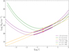 |
Fig. 5. Theoretical values of the ionization parameter U and the computed column density NH from Nion as derived from Eq. (4) (see Sect. 3.3). Solid and dashed lines correspond to the values of NH derived using Cfmin and Cfmax, respectively. The purple curves show the NH constraint from CIV, while the green and orange curves represent the upper limits from NV and Lyα, respectively. Bold lines indicate the allowed solutions for NH and U, while the red crosses mark the median values of the solutions adopted in Eq. (5). |
4. X-ray properties of SMSS J2157
4.1. XMM-Newton data reduction
SMSS J2157 has been observed in the X-rays with one exposure of 78.5 ks (Obs ID: 0844020101; PI. L. Zappacosta) with the observatory XMM-Newton, on 24–25 October 2019. The observation was reduced with the Science Analysis System (SAS) version 19.1.0 following the standard science threads. Time intervals characterized by highly variable high-energy background flares in the EPIC pn and MOS cameras were selected and removed. Specifically, we considered good time intervals for scientific analysis only those having pn, MOS1 and MOS2 count rates ≤0.4 counts/s (in the 10 − 12 keV band), ≤0.17 counts/s (> 10 keV) and ≤0.24 counts/s (> 10 keV), respectively. We performed for each camera source spectral extraction on circular regions centered on the QSO optical position. The background region on the pn camera was chosen as a rectangular region around the source with roughly the same position angle as the observation and with short and long sides of ∼2.3 and ∼3.7 arcmin, while on the MOS cameras was taken to be a circular region centered on the QSO position with radius ∼2.5 arcmin. The extraction of the background spectra was performed on these regions excluding circular regions of radius 40–50 arcsec (according to the source flux) centered on the position of all X-ray point-like sources (including the target QSO). The pn and MOS spectra were binned following the Kaastra & Bleeker (2016) optimization scheme which ensures high accuracy in recovering the true source spectral parameters regardless of the analysis energy interval adopted (Zappacosta et al. 2023).
4.2. X-ray spectral fitting results
The EPIC spectra were analyzed in the 0.3–10 keV energy band (corresponding to a rest-frame energy range of ∼2 − 50 keV) with the XSPEC v.12.11.1 spectral fitting package. We performed spectral modeling adopting the Cash statistics, as implemented in XSPEC with the direct background subtraction (W-stat in XSPEC Cash 1979; Wachter et al. 1979). In this energy band, the pn, MOS1, and MOS2 spectra consist of 169, 78, and 77 background subtracted counts, respectively. We modeled the X-ray spectrum with a power-law model modified by Galactic column density of 1.14 × 1020 cm−2 (HI4PI Collaboration 2016), yielding a photon index of Γ = 1.52 ± 0.11 and a fit statistic of W − stat = 259 for 205 degrees of freedom (d.o.f.). This parametrization shows a significant excess at ∼1 − 2 keV and negative residuals elsewhere, especially at low (< 0.9 keV) energies. Therefore, in the fitting model we included an additional cold absorption component, parametrized by the model ztbabs in XSPEC, accounting for the intrinsic obscuration at the quasar rest-frame. We obtained a best-fit model with W − stat/d.o.f. = 249/204 and a better description of the data in terms of residuals (see Fig. 6, left panel). We found a best-fit  with an intrinsic column density of
  , corresponding to an observed flux of 8.3
 × 10−15 erg cm−2 s−1 in the 2–10 keV band. This implies an intrinsic 2–10 keV luminosity
  . Given the rest-frame high energy probed by this XMM-Newton observation, we also included an additive term accounting for Compton reflection (not modified by the QSO intrinsic absorber) due to primary coronal X-rays reflected from circumnuclear cold material which typically peaks at 20–30 keV, by adopting the XSPEC model pexrav (Magdziarz & Zdziarski 1995). In this fit, we had to fix the power-law continuum slope to Γ = 2 because of the strong degeneracy among other free parameters. The best-fit model resulted in a negligible reflection component with a reflection strength of R < 0.05. This is in agreement with the findings reported of other luminous QSOs, which typically show a very weak reflection component (e.g., Reeves & Turner 2000; Zappacosta et al. 2018).
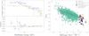 |
Fig. 6. Top-left panel: X-ray EPIC spectra (data) and relative best-fit power-law models modified by intrinsic absorption (dashed lines) and in the lower plot the residuals, i.e., data minus best-fit models. Blue, green, and orange colors refer to the pn, MOS1, and MOS2 detectors, respectively. Energies are reported at the rest-frame. Right panel: αox vs L2500. SMSS J2157 is reported as green star, while green, red and blue colors indicate a compilation of type 1 AGNs (Lusso & Risaliti 2016), bright UV-selected quasars (Nardini et al. 2019), and optically/IR selected bright QSOs from the WISSH sample (Zappacosta et al. 2020), respectively. Solid and dashed black lines report the relations inferred by Lusso & Risaliti (2016) and Martocchia et al. (2017). |
The value of the X-ray continuum slope is consistent with that expected from the λEdd ∼ 0.4 of SMSS J2157 according to the most recent Γ-λEdd relations (Liu et al. 2021; Laurenti et al. 2024). The presence of a large amount of X-ray absorption (NH ≈ 1023 cm−2) along our line of sight to the nucleus is also typically observed in the vast majority of BAL quasars at any redshift (e.g., Gallagher et al. 2002; Piconcelli et al. 2005; Martocchia et al. 2017).
Adopting the intrinsically absorbed power-law model as our fiducial best fit for the X-ray spectrum of SMSS J2157, we measured a monochromatic 2 keV luminosity of 3.16 × 1027 erg/s/Hz, which implies an optical-to-X-ray spectral index (a measurement of the strength of the ionizing SED)  /L2500Å) = −2.03. The right panel of Fig. 6 shows that this value lies below the well-established αOX-L2500Å relations for active galactic nuclei (AGNs). Specifically, we calculated a Δ(αOX) ≈ −0.2 corresponding to the difference of the αOX found for SMSS J2157 with respect to the expected value of αOX from the Lusso & Risaliti (2016) relation. Such a Δ(αOX) is typically considered the threshold for a source to be classified as intrinsically X-ray weak (Luo et al. 2015; Zappacosta et al. 2020). The X-ray bolometric correction of
  /L2 − 10 = 2.29 × 1048/2.34 × 1045 ≈ 980 is a factor of ∼2 larger than the
  derived by assuming the
  -LBol relation derived by Duras et al. (2020) for type 1 AGN. Both pieces of evidence therefore lend support to the notion that SMSS J2157 could be an intrinsically X-ray-weak-like QSO. This is not particularly surprising since there is growing store of literature reporting a sizable fraction (∼30%) of sources at the brightest end of the AGN luminosity function (
 ) exhibiting a significantly weaker X-ray emission than other QSO at comparable LBol (e.g., Nardini et al. 2019; Zappacosta et al. 2020).
BAL QSOs tend to be weaker in X-rays than non-BAL QSOs (e.g., Saccheo et al. 2023), with softer SEDs, indicated by steeper αOX. Another indicator of the strength of the ionizing SED is the He IIλ1640 emission line, a recombination line from He III. Its intensity directly reflects the number of photons with energies above 54.4 eV, serving as a proxy for the ionizing EUV. The weakness of He II emission in SMSS J2157 spectrum (see Fig. 1) is consistent with our findings of soft X-ray continuum, as it prevents the overionization of the high-velocity outflow; meanwhile the UV radiation accelerates the BAL outflow to high velocities (e.g., Murray et al. 1995). Furthermore, by recovering the CIV emission line velocity shift (as derived in Sect. 2.2), SMSS J2157 follows the relation found by Zappacosta et al. (2020) between αox and the CIV shift. The largest shifts are exhibited by X-ray weak sources, where the launch of fast winds is favored by reduced X-ray emission.
5. Kinematics and energetics of the EHVO outflow
Our results indicate that SMSS J2157 shows a persistent outflow with no variation over a few months to one year, with a maximum velocity of vmax ∼ 0.13c. This is consistent with reports that over such short timescales (i.e., ∼0.06–0.2 years), more than 90% of BALs do not show any time variations (Capellupo et al. 2013) and the expected amplitude of variation is very small, even if they are variable (see Fig. 11 of Gibson et al. 2008).
Fiore et al. 2017 found a strong correlation between AGN bolometric luminosity and maximum velocity for X-ray UFOs, BALs and lower velocity X-ray absorbers. Similarly, Matzeu et al. (2023) found a correlation by analyzing X-ray UFOs from the SUBWAYS sample at intermediate redshift and incorporating low- and high-redshift UFOs in their comprehensive study. Surprisingly, no clear dependence is reported for EHVOs, as shown in Fig. 7. The EHVO data from RH20203, along with data from Bischetti et al. (2022) and the WISSH QSOs J0947+1421 and J1538+0855 (Bruni et al. 2019; Vietri et al. 2022), are presented in the figure. Although SMSS J2157 is the most luminous source, its outflow velocity remains within the typical range observed for other EHVOs.
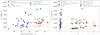 |
Fig. 7. Velocity of different types of outflows as a function of LBol (left panel) and redshift (right panel). The green star symbol denotes the EHVO outflow of SMSS J2157 with vout = vmax. High-redshift BALs and EHVOs from Bischetti et al. (2022) are represented as empty red circles. EHVOs from RH20 are shown as orange filled stars, while EHVOs from Vietri et al. (2022) and Bruni et al. (2019) are indicated by filled and empty magenta stars, respectively. The collection of X-ray UFOs from Fiore et al. (2017) and Matzeu et al. (2023) (SUBWAYS sample) is reported as blue and magenta triangles, respectively. In the right panel, BAL from Bischetti et al. (2023) are also shown as purple filled circles. The velocity threshold of 25 000 km/s, which distinguishes between classical low-velocity BALs and EHVOs, is shown as a red dashed line. |
Notably, the parameter space for these outflows is confined to a high-luminosity regime, spanning approximately one order of magnitude, and does not extend to the highest velocities seen in X-ray UFOs (compiled from Fiore et al. 2017 and the SUBWAYS sample from Matzeu et al. 2023). The latter, in contrast, are observed across nearly three orders of magnitude in luminosity.
Bischetti et al. (2023) observed that the velocity of classical BAL outflows (v ≤ 25 000 km s−1) generally increases with redshift, suggesting that in the high-redshift universe, BAL outflows may be more readily accelerated to EHVOs compared to later cosmic epochs, with velocities observed up to v ∼ 55 000 km s−1 (Bischetti et al. 2022). Such EHVOs observed at early cosmic epochs are also found at lower redshifts, as illustrated in Fig. 7 (right panel). This suggests that EHVOs maintain very high velocities throughout cosmic time, with values consistent with the results reported at high redshift by Bischetti et al. (2022). However, a more comprehensive and systematic study of EHVOs across a wider redshift range is needed to draw more robust and reliable conclusions.
Using the physical parameters of the EHVO reported in Sect. 3.3, the outflow kinetic power can be constrained with assumptions. A key method to reduce uncertainties in these estimates is spectral variability analysis, which helps constrain the outflow distance. However, since no spectral variation is observed in the multi-epoch spectra, this method cannot be applied to estimate the distance of the EHVO from the BH.
Therefore, we adopted the BLR radius RBLR ∼ 0.35 pc (Lira et al. 2018), as the location of the EHVO. This choice provides a conservative lower limit on the outflow’s distance. By assuming an expanding shell at a certain velocity (vEHVO = vmax) and at a radial distance, REHVO = RBLR, the kinetic energy can be expressed as
 (5)
(5)
with Q = 0.15 (based on the incidence of CIV BALs in SDSS QSOs, e.g., Gibson et al. 2009; Hamann et al. 2019) and NHCfmax = 2.8 × 1020 cm−2 and NHCfmin = 1.1 × 1021 cm−2, as derived in Sect. 3.3. Dividing EK, EHVO by a characteristic flow time given by REHVO/vmax, we find a conservative range for the kinetic power of  ∼ 3.6 × 1043 erg/s and
  ∼ 1.45 × 1044 erg/s4.
The mass outflow rate is ∼0.06 (0.25) M⊙ yr−1, for Cfmax (Cfmin). Assuming a mass to radiation conversion efficiency of η ∼ 0.1, the mass outflow rate corresponds to about 0.02% (0.06%) of the mass accretion rate (∼400 M⊙ yr−1), for Cfmax (Cfmin).
The kinetic power for SMSS J2157 is ∼0.002% (0.006%) of the bolometric luminosity, for Cfmax (Cfmin) (see Fig. 8). These values are below to what is found for X-ray UFO and BAL as found by Fiore et al. 2017 and for X-ray UFOs from the SUBWAYS sample by Gianolli et al. 2024. As shown in Fig. 8, about half of the X-ray absorbers and BAL winds have ĖK/LBol in the range of 1–10% with another half having ĖK/LBol < 1%. However, X-ray UFOs are usually identified in AGNs with moderate luminosities (LBol ∼ 1043 − 46.5 erg/s); therefore, under similar physical conditions (high outflow velocities and large column densities), they can more easily reach higher values of ĖK/LBol. In contrast, for very luminous quasars like SMSS J2157, the same absolute kinetic power corresponds to a much lower fraction of the bolometric output.
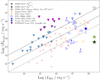 |
Fig. 8. Distribution of ĖK,out as a function of LBol for different types of outflows. The dotted, dot-dashed, and dashed lines indicate the thresholds of 0.1, 1, and 10 percent, respectively. The dark and light green star symbols denote the EHVO outflow of SMSS J2157 as reported in this paper by adopting NHCfmin and NHCfmax, respectively, while the empty star represents ĖK,out obtained by adopting NH = 1022 cm−2 and REHVO = 100 pc, values generally derived using VHP outflows and excited states, respectively (see Sect. 5 for a detailed discussion). Other symbols denote the parameters of X-ray (blue triangles), ionized (red crosses), and BAL outflow (orange stars) reported by Fiore et al. (2017), SUBWAYS X-ray UFO from Gianolli et al. (2024), BAL reported by Miller et al. (2020) (right-pointing triangles), and EHVO from Vietri et al. (2022) (blue star). |
Moreover, various factors of uncertainty in NH and REHVO can impact the outflow energetics measurement. Arav et al. (2013) identified two distinct ionization phases in quasar outflows, high-potential (HP) and very-high potential (VHP) outflow, observed in all outflows at λrest ≥ 1050 Å and in the range 500–1050 λ rest-frame (EUV500), respectively. The VHP exhibits an NH that is 5–100 times larger than that of the HP (Arav et al. 2020), corresponding to ĖK,EHVO values that are one to two orders of magnitude higher. Therefore, deriving the parameters of the VHP is crucial for understanding the impact of outflows on the host galaxy. As stated in Arav et al. (2020) it is probable that the large majority of HP outflows observed at λrest ≥ 1050 Å (as those observed in CIV line of SMSS J2157) also have an associated VHP outflow, with a derived column density which can yield measurements even larger than NH = 1022 cm−2. This is more than ∼1 dex larger than the one derived for our target.
A robust way to derive REHVO is through the use of transitions from excited states. However these transitions are mostly observable in the EUV500 wavelength range, which is affected by Lyα forest at high redshift. Using this method, previous studies have found a distance of hundreds of pc (e.g., Arav et al. 2020), approximately three orders of magnitude larger than our conservative lower limit assuming a sub-pc BLR location. Therefore, by adopting values typically derived using VHP outflows and excited states, such as NH = 1022 cm−2 and REHVO = 100 pc, we obtain ĖK,EHVO = 3.7 × 1047 erg/s (∼16% LBol).
As a result, ĖK,EHVO can reach values potentially capable of delivering efficient feedback to the host galaxy’s interstellar medium (based on Hopkins & Elvis (2010), where ∼0.5% of the bolometric luminosity is typically adopted as the threshold for effective AGN feedback via outflows).
6. Summary and conclusions
We present a detailed spectroscopic study of SMSS J2157, the most luminous QSO in the first 1.3 Gyr, based on multi-epoch observations with VLT/XSHOOTER, as well as combined Keck/NIRES and VLT/XSHOOTER data. In this study, we report the discovery of a persistent EHVO in SMSS J2157. Our main findings can be summarized as follows:
-
Properties of the EHVO in absorption: the EHVO outflow displays a CIV balnicity index BI
 km s−1, which is among the largest values discovered so far for EHVOs with velocities exceeding 35 000 km s−1. It also shows a stable maximum velocity of vmax ∼ 42 350 km s−1 (∼0.13c) over a monitoring period of months to a year. The NV and Lyα EHVO components at similar velocities are also detected, although they are blended with the Lyα forest.
 -
Properties of the CIV emission line: we found an EW(CIV) ∼17 ± 2 Å, placing it marginally within the weak emission line regime as defined by Chen et al. (2024), with
 ± 200 km/s, indicating a strong BLR outflow. These properties are consistent with the findings of low equivalent widths and significant blueshifts in the CIV emission line observed in a sample of EHVOs analyzed by Rodríguez Hidalgo & Rankine 2022.
 -
X-ray spectral properties: SMSS J2157 exhibits a steep optical-to-X-ray spectral index (αOX = −2.03) along with a significant X-ray bolometric correction, classifying it as a X-ray-weak-like source that is typical of BAL QSOs. The source follows the αOX versus blueshift relation for the hyperluminous quasars reported by Zappacosta et al. 2020. The observed weakness may play a critical role in preventing overionization of the innermost disk atmosphere, thereby allowing an efficient launch of the fastest nuclear UV outflows such as the EHVO presented in this work.
-
Energetics of the EHVO: our estimates place a conservative range of values of the kinetic power of the outflow at
 ∼ 3.6 × 1043 erg/s and
  ∼ 1.45 × 1044 erg/s, for Cfmax and Cfmin, respectively. Given the extremely high bolometric luminosity of SMSS J2157, this corresponds to approximately 0.002% (0.006%) of the quasar’s radiative output, for Cfmax (Cfmin), significantly below the 0.5-5% of bolometric luminosity threshold typically considered necessary for efficient AGN feedback mechanisms. However, this value reflects conservative assumptions on the outflow location and uncertainties in the column density (see Sect. 5).
Our findings suggest that EHVOs may be a common feature of luminous QSOs across all redshifts and, in turn, they could provide an efficient feedback mechanism for the co-evolution of galaxies hosting highly accreting, massive SMBHs. Future monitoring campaigns are needed to confirm the persistence of the outflow over timescales of several years. In addition, any variability, if detected, can provide stringent constraints on the outflow’s location, ultimately reducing uncertainties in the kinetic power estimates.
We adopted the convention of using a positive sign for blueshifted line velocities, with respect to the MgII-based redshift (Onken et al. 2020).
Each analyzed doublet was constrained to have the correct separation and a 2:1 optical depth ratio between the short- and long-wavelength components.
The gap in the velocity distribution between ∼25 000 and ∼30 000 km s−1 arises from the selection strategy adopted in the search for EHVOs in RH2020, aimed at avoiding contamination from the SiIV+OIV] emission line complex.
By adopting equations (9) and (11) from Dunn et al. (2010) for Ṁout and ĖK,EHVO, respectively, with a mean molecular weight μ = 1.4, we obtain values approximately 2.8 times higher than those derived in Sect. 5.
Acknowledgments
We thank the anonymous referee for the useful comments that improved the paper. We warmly thank Wendy F. García Naranjo and Tzitzi Romo Pérez for their contribution to the initial stages of the fitting code used to deconvolve the SiIV and CIV absorption features. We are also grateful to Vittoria Gianolli for kindly providing us with data from the SUBWAYS sample. Based on observations collected at the European Southern Observatory under ESO programme 0103.B-0949(A). G. V. acknowledges financial support from the Bando Ricerca Fondamentale INAF 2022 Mini-grant “Searching for UV ultra-fast outflow in AGN by exploiting widearea public spectroscopic surveys” and INAF 2023 Guest Observer Grant “Assessing the role of ultra-fast outflows in hyper-luminous quasars at Cosmic Noon”. P.R.H. and L.F. acknowledge support from the National Science Foundation AAG Award AST-2107960, the Sloan Digital Sky Survey’s Faculty And Student Team program, funded by the Alfred P. Sloan Foundation, and the Mary Gates research scholarship program. EP acknowledges funding from the European Union – Next Generation EU, PRIN/MUR 2022 2022K9N5B4. T.M. acknowledges support from JSPS KAKENHI Grant Number 25K01038. ALR acknowledges support from a UKRI Future Leaders Fellowship (grant code: MR/T020989/1). LZ acknowledges financial support from the Bando Ricerca Fondamentale INAF 2022 Large Grant “Toward an holistic view of the Titans: multi-band observations of z > 6 QSOs powered by greedy supermassive black holes” and from the European Union – Next Generation EU, PRIN/MUR 2022 2022TKPB2P – BIG-z. For the purpose of open access, the author has applied a Creative Commons Attribution (CC BY) licence to any Author Accepted Manuscript version arising from this submission.
References
- Allen, J. T., Hewett, P. C., Richardson, C. T., Ferland, G. J., & Baldwin, J. A. 2013, MNRAS, 430, 3510 [NASA ADS] [CrossRef] [Google Scholar]
- Arav, N., de Kool, M., Korista, K. T., et al. 2001, ApJ, 561, 118 [NASA ADS] [CrossRef] [Google Scholar]
- Arav, N., Borguet, B., Chamberlain, C., Edmonds, D., & Danforth, C. 2013, MNRAS, 436, 3286 [NASA ADS] [CrossRef] [Google Scholar]
- Arav, N., Xu, X., Miller, T., Kriss, G. A., & Plesha, R. 2020, ApJS, 247, 37 [Google Scholar]
- Bischetti, M., Feruglio, C., D’Odorico, V., et al. 2022, Nature, 605, 244 [NASA ADS] [CrossRef] [Google Scholar]
- Bischetti, M., Fiore, F., Feruglio, C., et al. 2023, ApJ, 952, 44 [NASA ADS] [CrossRef] [Google Scholar]
- Blustin, A. J., Page, M. J., Fuerst, S. V., Branduardi-Raymont, G., & Ashton, C. E. 2005, A&A, 431, 111 [CrossRef] [EDP Sciences] [Google Scholar]
- Bock, D. C.-J., Large, M. I., & Sadler, E. M. 1999, ApJ, 117, 1578 [Google Scholar]
- Boquien, M., Burgarella, D., Roehlly, Y., et al. 2019, A&A, 622, A103 [NASA ADS] [CrossRef] [EDP Sciences] [Google Scholar]
- Bruni, G., Piconcelli, E., Misawa, T., et al. 2019, A&A, 630, A111 [NASA ADS] [CrossRef] [EDP Sciences] [Google Scholar]
- Capellupo, D. M., Hamann, F., Shields, J. C., Halpern, J. P., & Barlow, T. A. 2013, MNRAS, 429, 1872 [CrossRef] [Google Scholar]
- Carnall, A. C. 2017, arXiv e-prints [arXiv:1705.05165] [Google Scholar]
- Cash, W. 1979, ApJ, 228, 939 [Google Scholar]
- Chatzikos, M., Bianchi, S., Camilloni, F., et al. 2023, Rev. Mex. Astron. Astrofis., 59, 327 [Google Scholar]
- Chen, Y., Luo, B., Brandt, W. N., et al. 2024, ApJ, 972, 191 [Google Scholar]
- Condon, J. J., Cotton, W. D., Greisen, E. W., et al. 1998, ApJ, 115, 1693 [Google Scholar]
- Crenshaw, D. M., Kraemer, S. B., & George, I. M. 2003, ARA&A, 41, 117 [NASA ADS] [CrossRef] [Google Scholar]
- Devillard, N. 1997, The Messenger, 87, 19 [NASA ADS] [Google Scholar]
- Dunn, J. P., Bautista, M., Arav, N., et al. 2010, ApJ, 709, 611 [NASA ADS] [CrossRef] [Google Scholar]
- Duras, F., Bongiorno, A., Ricci, F., et al. 2020, A&A, 636, A73 [NASA ADS] [CrossRef] [EDP Sciences] [Google Scholar]
- Fiore, F., Feruglio, C., Shankar, F., et al. 2017, A&A, 601, A143 [NASA ADS] [CrossRef] [EDP Sciences] [Google Scholar]
- Foreman-Mackey, D., Farr, W., Sinha, M., et al. 2019, J. Open Source Software, 4, 1864 [CrossRef] [Google Scholar]
- Gallagher, S. C., Brandt, W. N., Chartas, G., & Garmire, G. P. 2002, ApJ, 567, 37 [CrossRef] [Google Scholar]
- Gianolli, V. E., Bianchi, S., Petrucci, P. O., et al. 2024, A&A, 687, A235 [NASA ADS] [CrossRef] [EDP Sciences] [Google Scholar]
- Gibson, R. R., Brandt, W. N., Schneider, D. P., & Gallagher, S. C. 2008, ApJ, 675, 985 [NASA ADS] [CrossRef] [Google Scholar]
- Gibson, R. R., Brandt, W. N., Gallagher, S. C., & Schneider, D. P. 2009, ApJ, 696, 924 [NASA ADS] [CrossRef] [Google Scholar]
- Hamann, F., & Ferland, G. 1999, ARA&A, 37, 487 [Google Scholar]
- Hamann, F., Herbst, H., Paris, I., & Capellupo, D. 2019, MNRAS, 483, 1808 [NASA ADS] [CrossRef] [Google Scholar]
- Henden, A. A., Templeton, M., Terrell, D., et al. 2016, VizieR Online Data Catalog: AAVSO Photometric All Sky Survey (APASS) DR9 (Henden+, 2016), VizieR On-line Data Catalog: II/336. Originally published. In: 2015AAS.22533616H [Google Scholar]
- HI4PI Collaboration (Ben Bekhti, N., et al.) 2016, A&A, 594, A116 [NASA ADS] [CrossRef] [EDP Sciences] [Google Scholar]
- Højen-Sørensen, P. A., Winther, O., & Hansen, L. K. 2002, Neural Comput., 14, 889 [Google Scholar]
- Hopkins, P. F., & Elvis, M. 2010, MNRAS, 401, 7 [NASA ADS] [CrossRef] [Google Scholar]
- Kaastra, J. S., & Bleeker, J. A. M. 2016, A&A, 587, A151 [NASA ADS] [CrossRef] [EDP Sciences] [Google Scholar]
- King, A., & Pounds, K. 2015, ARA&A, 53, 115 [NASA ADS] [CrossRef] [Google Scholar]
- Komatsu, E., Smith, K. M., Dunkley, J., et al. 2011, ApJS, 192, 18 [Google Scholar]
- Lai, S., Wolf, C., Onken, C. A., & Bian, F. 2023, MNRAS, 521, 3682 [Google Scholar]
- Laurenti, M., Tombesi, F., Vagnetti, F., et al. 2024, A&A, 689, A337 [NASA ADS] [CrossRef] [EDP Sciences] [Google Scholar]
- Lira, P., Kaspi, S., Netzer, H., et al. 2018, ApJ, 865, 56 [NASA ADS] [CrossRef] [Google Scholar]
- Liu, H., Luo, B., Brandt, W. N., et al. 2021, ApJ, 910, 103 [Google Scholar]
- Lodders, K. 2003, ApJ, 591, 1220 [Google Scholar]
- Luminari, A., Piconcelli, E., Tombesi, F., Nicastro, F., & Fiore, F. 2024, A&A, 691, A357 [NASA ADS] [CrossRef] [EDP Sciences] [Google Scholar]
- Luo, B., Brandt, W. N., Hall, P. B., et al. 2015, ApJ, 805, 122 [Google Scholar]
- Lusso, E., & Risaliti, G. 2016, ApJ, 819, 154 [Google Scholar]
- Lusso, E., Comastri, A., Vignali, C., et al. 2010, A&A, 512, A34 [NASA ADS] [CrossRef] [EDP Sciences] [Google Scholar]
- Magdziarz, P., & Zdziarski, A. A. 1995, MNRAS, 273, 837 [Google Scholar]
- Martocchia, S., Piconcelli, E., Zappacosta, L., et al. 2017, A&A, 608, A51 [NASA ADS] [CrossRef] [EDP Sciences] [Google Scholar]
- Matzeu, G. A., Brusa, M., Lanzuisi, G., et al. 2023, A&A, 670, A182 [Google Scholar]
- McMahon, R. G., Banerji, M., Gonzalez, E., et al. 2013, The Messenger, 154, 35 [NASA ADS] [Google Scholar]
- Miller, T. R., Arav, N., Xu, X., & Kriss, G. A. 2020, MNRAS, 499, 1522 [NASA ADS] [CrossRef] [Google Scholar]
- Misawa, T., Charlton, J. C., Eracleous, M., et al. 2007, ApJS, 171, 1 [NASA ADS] [CrossRef] [Google Scholar]
- Modigliani, A., Goldoni, P., Royer, F., et al. 2010, in Observatory Operations: Strategies, Processes, and Systems III, eds. D. R. Silva, A. B. Peck, & B. T. Soifer, SPIE Conf. Ser., 7737, 773728 [NASA ADS] [CrossRef] [Google Scholar]
- Murray, N., Chiang, J., Grossman, S. A., & Voit, G. M. 1995, ApJ, 451, 498 [NASA ADS] [CrossRef] [Google Scholar]
- Nardini, E., Lusso, E., Risaliti, G., et al. 2019, A&A, 632, A109 [NASA ADS] [CrossRef] [EDP Sciences] [Google Scholar]
- Onken, C. A., Bian, F., Fan, X., et al. 2020, MNRAS, 496, 2309 [NASA ADS] [CrossRef] [Google Scholar]
- Opper, M., & Winther, O. 2005, J. Mach. Learn. Res., 6, 2177 [Google Scholar]
- Piconcelli, E., Jimenez-Bailón, E., Guainazzi, M., et al. 2005, A&A, 432, 15 [NASA ADS] [CrossRef] [EDP Sciences] [Google Scholar]
- Polletta, M., Tajer, M., Maraschi, L., et al. 2007, ApJ, 663, 81 [NASA ADS] [CrossRef] [Google Scholar]
- Prevot, M. L., Lequeux, J., Maurice, E., Prevot, L., & Rocca-Volmerange, B. 1984, A&A, 132, 389 [Google Scholar]
- Rankine, A. L., Hewett, P. C., Banerji, M., & Richards, G. T. 2020, MNRAS, 492, 4553 [CrossRef] [Google Scholar]
- Reeves, J. N., & Turner, M. J. L. 2000, MNRAS, 316, 234 [NASA ADS] [CrossRef] [Google Scholar]
- Rodríguez Hidalgo, P., & Rankine, A. L. 2022, ApJ, 939, L24 [CrossRef] [Google Scholar]
- Rodríguez Hidalgo, P., Hamann, F., & Hall, P. 2011, MNRAS, 411, 247 [CrossRef] [Google Scholar]
- Rodríguez Hidalgo, P., Khatri, A. M., Hall, P. B., et al. 2020, ApJ, 896, 151 [CrossRef] [Google Scholar]
- Rogerson, J. A., Hall, P. B., Rodríguez Hidalgo, P., et al. 2016, MNRAS, 457, 405 [NASA ADS] [CrossRef] [Google Scholar]
- Saccheo, I., Bongiorno, A., Piconcelli, E., et al. 2023, A&A, 671, A34 [NASA ADS] [CrossRef] [EDP Sciences] [Google Scholar]
- Schlafly, E. F., & Finkbeiner, D. P. 2011, ApJ, 737, 103 [Google Scholar]
- Shen, Y., Richards, G. T., Strauss, M. A., et al. 2011, ApJS, 194, 45 [Google Scholar]
- Skrutskie, M. F., Cutri, R. M., Stiening, R., et al. 2006, AJ, 131, 1163 [NASA ADS] [CrossRef] [Google Scholar]
- Smette, A., Sana, H., Noll, S., et al. 2015, A&A, 576, A77 [NASA ADS] [CrossRef] [EDP Sciences] [Google Scholar]
- Tombesi, F., Cappi, M., Reeves, J. N., et al. 2010, A&A, 521, A57 [NASA ADS] [CrossRef] [EDP Sciences] [Google Scholar]
- Tombesi, F., Cappi, M., Reeves, J. N., & Braito, V. 2012, MNRAS, 422, L1 [Google Scholar]
- Vernet, J., Dekker, H., D’Odorico, S., et al. 2011, A&A, 536, A105 [NASA ADS] [CrossRef] [EDP Sciences] [Google Scholar]
- Vietri, G., Misawa, T., Piconcelli, E., et al. 2022, A&A, 668, A87 [NASA ADS] [CrossRef] [EDP Sciences] [Google Scholar]
- Wachter, K., Leach, R., & Kellogg, E. 1979, ApJ, 230, 274 [NASA ADS] [CrossRef] [Google Scholar]
- Weymann, R. J., Morris, S. L., Foltz, C. B., & Hewett, P. C. 1991, ApJ, 373, 23 [NASA ADS] [CrossRef] [Google Scholar]
- Wilson, J. C., Henderson, C. P., Herter, T. L., et al. 2004, in Ground-based Instrumentation for Astronomy, eds. A. F. M. Moorwood, & M. Iye, SPIE Conf. Ser., 5492, 1295 [Google Scholar]
- Wolf, C., Bian, F., Onken, C. A., et al. 2018, PASA, 35, e024 [Google Scholar]
- Wright, E. L., Eisenhardt, P. R. M., Mainzer, A. K., et al. 2010, AJ, 140, 1868 [Google Scholar]
- Zappacosta, L., Comastri, A., Civano, F., et al. 2018, ApJ, 854, 33 [Google Scholar]
- Zappacosta, L., Piconcelli, E., Giustini, M., et al. 2020, A&A, 635, L5 [NASA ADS] [CrossRef] [EDP Sciences] [Google Scholar]
- Zappacosta, L., Piconcelli, E., Fiore, F., et al. 2023, A&A, 678, A201 [NASA ADS] [CrossRef] [EDP Sciences] [Google Scholar]
Appendix A: CIV blended-NALs
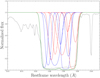 |
Fig. A.1. Normalized coadded spectrum of SMSS J2157 in the wavelength range of the CIV blended-NALs shown together with its best-fit model (green curve) and six pairs of Gaussian components (blue and red) modeling the doublets (see Sect. 2.3 for more details). |
All Tables
All Figures
|
Fig. 1. Final coadded spectrum of SMSS J2157, with the CIV, NV, and Lyα EHVO highlighted in light red. The blended NALs systems are indicated in aquamarine. The AlIII+CIII] and MgII emission lines are also marked. Regions affected by telluric absorption are marked in light grey. |
| In the text | |
|
Fig. 2. Median spectral reconstruction (black) created from the reconstructions with different parameters used in the spectral fitting. The original spectrum is plotted in grey. The regions affected by telluric absorption are marked as light grey color. |
| In the text | |
|
Fig. 3. Normalized, coadded spectrum of SMSS J2157, overlaid with the best-fit model (red curve) for the EHVO features of the CIV doublet (three blue-red pairs of dashed Gaussian components for modeling 1548,1550 Å lines respectively), NV doublet (three blue-red pairs of dotted Gaussian curves for modeling 1238,1242 Å lines respectively), Lyα (three blue dash-dotted Gaussian curves), and SiIV doublet blended NALs (seven green-purple pairs of dotted Gaussian components for modeling 1393,1402 Å lines, respectively). The spectrum was normalized to the reconstructed model at λ > 1275 Å and to the extrapolated continuum λ < 1275 Å. |
| In the text | |
|
Fig. 4. Best-fit de-reddened and reddened SEDs with 1σ errors for SMSS J2157 (purple and pink lines, respectively), as derived in Sect. 3.2. The 1 keV luminosity is shown as a left-pointing coral red triangle; REM/ROS2 g, r, i, z data are represented by orange circles; Y, J, and Ks points from VISTA are shown as down-pointing green triangles; the H point from 2MASS is represented by a down-pointing blue triangle; and golden yellow squares represent the W1-W4 WISE channels. The uncertainties of data points are shown but are smaller than the symbol size. |
| In the text | |
|
Fig. 5. Theoretical values of the ionization parameter U and the computed column density NH from Nion as derived from Eq. (4) (see Sect. 3.3). Solid and dashed lines correspond to the values of NH derived using Cfmin and Cfmax, respectively. The purple curves show the NH constraint from CIV, while the green and orange curves represent the upper limits from NV and Lyα, respectively. Bold lines indicate the allowed solutions for NH and U, while the red crosses mark the median values of the solutions adopted in Eq. (5). |
| In the text | |
|
Fig. 6. Top-left panel: X-ray EPIC spectra (data) and relative best-fit power-law models modified by intrinsic absorption (dashed lines) and in the lower plot the residuals, i.e., data minus best-fit models. Blue, green, and orange colors refer to the pn, MOS1, and MOS2 detectors, respectively. Energies are reported at the rest-frame. Right panel: αox vs L2500. SMSS J2157 is reported as green star, while green, red and blue colors indicate a compilation of type 1 AGNs (Lusso & Risaliti 2016), bright UV-selected quasars (Nardini et al. 2019), and optically/IR selected bright QSOs from the WISSH sample (Zappacosta et al. 2020), respectively. Solid and dashed black lines report the relations inferred by Lusso & Risaliti (2016) and Martocchia et al. (2017). |
| In the text | |
|
Fig. 7. Velocity of different types of outflows as a function of LBol (left panel) and redshift (right panel). The green star symbol denotes the EHVO outflow of SMSS J2157 with vout = vmax. High-redshift BALs and EHVOs from Bischetti et al. (2022) are represented as empty red circles. EHVOs from RH20 are shown as orange filled stars, while EHVOs from Vietri et al. (2022) and Bruni et al. (2019) are indicated by filled and empty magenta stars, respectively. The collection of X-ray UFOs from Fiore et al. (2017) and Matzeu et al. (2023) (SUBWAYS sample) is reported as blue and magenta triangles, respectively. In the right panel, BAL from Bischetti et al. (2023) are also shown as purple filled circles. The velocity threshold of 25 000 km/s, which distinguishes between classical low-velocity BALs and EHVOs, is shown as a red dashed line. |
| In the text | |
|
Fig. 8. Distribution of ĖK,out as a function of LBol for different types of outflows. The dotted, dot-dashed, and dashed lines indicate the thresholds of 0.1, 1, and 10 percent, respectively. The dark and light green star symbols denote the EHVO outflow of SMSS J2157 as reported in this paper by adopting NHCfmin and NHCfmax, respectively, while the empty star represents ĖK,out obtained by adopting NH = 1022 cm−2 and REHVO = 100 pc, values generally derived using VHP outflows and excited states, respectively (see Sect. 5 for a detailed discussion). Other symbols denote the parameters of X-ray (blue triangles), ionized (red crosses), and BAL outflow (orange stars) reported by Fiore et al. (2017), SUBWAYS X-ray UFO from Gianolli et al. (2024), BAL reported by Miller et al. (2020) (right-pointing triangles), and EHVO from Vietri et al. (2022) (blue star). |
| In the text | |
|
Fig. A.1. Normalized coadded spectrum of SMSS J2157 in the wavelength range of the CIV blended-NALs shown together with its best-fit model (green curve) and six pairs of Gaussian components (blue and red) modeling the doublets (see Sect. 2.3 for more details). |
| In the text | |
Current usage metrics show cumulative count of Article Views (full-text article views including HTML views, PDF and ePub downloads, according to the available data) and Abstracts Views on Vision4Press platform.
Data correspond to usage on the plateform after 2015. The current usage metrics is available 48-96 hours after online publication and is updated daily on week days.
Initial download of the metrics may take a while.