| Issue |
A&A
Volume 704, December 2025
|
|
|---|---|---|
| Article Number | A169 | |
| Number of page(s) | 13 | |
| Section | Planets, planetary systems, and small bodies | |
| DOI | https://doi.org/10.1051/0004-6361/202555856 | |
| Published online | 11 December 2025 | |
Component-resolved light curve of the binary main-belt comet 288P/2006 VW139
Astronomical Observatory, Jagiellonian University,
Kraków,
Poland
★ Corresponding authors: This email address is being protected from spambots. You need JavaScript enabled to view it.
; This email address is being protected from spambots. You need JavaScript enabled to view it.
Received:
6
June
2025
Accepted:
13
October
2025
Abstract
Context. Over half of the cometary nuclei and a part of the asteroids that have been photographed so far by space missions or imaged by Doppler radar techniques appear to be bilobate or contact binary systems. The latest research on these objects shows that rotational fission and fragment reconnection can lead to reconfiguration, creating the next generation of bilobate bodies. In this context, Main-belt comet 288P, the only known double object of this class with components of comparable masses, appears to have successfully avoided reconfiguration or disassociation into a dynamically unbound pair and has become a wide asynchronous binary.
Aims. Our goal was to determine the physical parameters, such as sizes, shapes, and rotation periods, of both components of 288P to understand how this double asteroid formed and how it has evolved to obtain today’s very wide orbit. We also tried to confirm or deny the existence of a third component in a tight pair with the larger, slowly rotating fragment, as previously suggested.
Methods. We obtained a composite light curve of 288P by observing this object with the Gemini South and Keck II telescopes working in tandem. Through model analysis we separated this light curve into components, one for each fragment. We found their sidereal rotation periods and the most probable shapes and sizes. We analysed the angular momentum and energy balances and compared actual values with that expected at the moment of rotational splitting to check how much surplus has been introduced into the system.
Results. We determined the rotation periods of the components to be 15.86 hours for the larger object A and 3.37 hour for the smaller fragment B. Assuming a geometric albedo of 0.07 in the R photometric band, surface and reflectance properties adequate for C-type asteroids and comets, and considering A and B as prolate spheroids, we found that their semi-axes a, b (where b < a) are equal to 1.12, 0.69 and 0.67, 0.57 km for the larger and smaller components, respectively. The existence of a third body in 288P cannot be definitely excluded but should be considered as unlikely.
Conclusions. A plausible mechanism responsible for the origin of the binary asteroid 288P is rotational fission of a bilobate progenitor spun up by the Yarkovsky-O’Keefe-Radzievskii-Paddack mechanism or, more likely, by sublimation-driven torque produced by an active region or regions. It is almost certain that the sublimative activity of the smaller fragment B is behind its relatively fast, completely asynchronous rotation and the wide mutual orbit of the components.
Key words: minor planets / asteroids: individual: (300163) 2006 VW139 / comets: individual: 288P/2006 VW139
© The Authors 2025
 Open Access article, published by EDP Sciences, under the terms of the Creative Commons Attribution License (https://creativecommons.org/licenses/by/4.0), which permits unrestricted use, distribution, and reproduction in any medium, provided the original work is properly cited.
This article is published in open access under the Subscribe to Open model. This email address is being protected from spambots. You need JavaScript enabled to view it. to support open access publication.
1 Introduction
Main-belt comets (MBC), which belong to a subclass of active asteroids, are very unusual solar system bodies that have orbital parameters characteristic of main-belt asteroids but display protracted and recurrent cometary activity (Hsieh & Jewitt 2006). They revolve around the Sun inside the orbit of Jupiter (Tis-serand invariant TJ > 3) and from time to time show comet-like comae and tails. Their existence distorts the classical picture of the Solar System in which asteroids and comets comprise two physically different classes of objects. Whereas the building material for the former group are rocks, the latter constitute snowy remnants of the early formation stages of the planetary system. After years of research, it has become obvious that this simple dichotomy does not adequately describe reality and that we should rather speak about a continuum of cases from active comets to inactive asteroids. What is more, we may be dealing with a selection bias, as the limited sensitivity of our instruments makes it impossible to detect some active objects in the main belt (Jewitt & Hsieh 2024). Many processes that could explain the activity of MBCs have been proposed (Jewitt 2012) but those that have been most seriously taken into account are water ice sublimation or catastrophic impact. When the active phase is closely correlated with perihelion passage, we are dealing with ice sublimation from a fresh icy layer previously excavated by centrifugal or collisional disruption (e.g. Jewitt et al. 2015). Otherwise, if the mass loss is triggered unexpectedly and is uncorrelated with heliocentric distance, we can attribute such an event to a hypersonic impact (e.g. Bottke et al. 1994).
Main-belt comet 288P (known as numbered asteroid 300163, formerly 2006 VW 139) has a semi-major axis of 3.05 AU, hence it belongs to the outer asteroid belt. Its orbital eccentricity is equal to 0.20 and its inclination equals 3.24 deg. The activity of 288P was first discerned in 2011 by the Panoramic Survey Telescope and Rapid Response System (Pan-STARRS1) (Hsieh et al. 2012). Since that time it has shown typical recurrent activity around perihelion and an inactive phase at aphelion. This otherwise typical representative of MBCs was the first suspected of being a binary system (Agarwal et al. 2016). Further research confirmed that 288P is indeed a binary with component separation being at the resolution limit of the Hubble Space Telescope (HST) (Agarwal et al. 2017). Long lasting HST monitoring of 288P made it possible to estimate the parameters of the mutual orbit, which has a semi-major axis slightly over 100 km, an eccentricity close to 0.5, a period a little bit shorter than 120 days, and an orbital plane roughly aligned with the heliocentric orbit of the asteroid (Agarwal et al. 2020). What is more, the components appear to have comparable kilometer sizes, both are elongated, one more, the other less. Compared with other known binary asteroids, the relationship between the mutual semi-major axis and size ratio of the secondary to the primary makes 288P somewhat unique, due to its wide component separation and comparably sized fragments (see Fig. 3 of Agarwal et al. 2017). The limited resolution of the HST data makes it impossible to definitively determine whether both components were active or only one of them and, in that case, which one was active, although Agarwal et al. (2017) suggest that dust was emitted by the smaller B fragment. As was shown by Jacobson & Scheeres (2011), the largest possible distance between binary components, achieved after rotational fission of a strengthless progenitor and 100 years of evolution, is on the order of a few radii of the primary object for components of similar masses. This is many times smaller than the mean separation observed in 288P. There are therefore two main questions concerning this active asteroid: what mechanism created such an unusual binary MBC, and why is the separation between the components so large? Two reasons can theoretically explain the binarity of 288P: rotational break-up and catastrophic collision. If the binary nature of 288P is a result of rotational splitting of a bilobate body (Pravec & Harris 2007; Walsh et al. 2008) after its spinning up by the Yarkovsky–O’Keefe–Radzievskii–Paddack (YORP) effect (Rubincam 2000) for example, the only reasonable possibility to separate both fragments so much are non-gravitational forces generated by the radiative or sublimative binary YORP (BYORP) (Ćuk & Burns 2005; Jacobson et al. 2014), of which the latter is the preferred explanation (Agarwal et al. 2017). To effectively operate, BYORP needs at least partial locking of rotation and orbital motion by tidal interactions. On the other hand, if the system was created by a collision, then the wide separation of the components can be naturally understood within the escaping ejecta binaries (EEB) scenario (Durda et al. 2004). This scenario is quite possible as 288P itself could have originated from such an event about 7.5 Myr ago (Novaković et al. 2012). The co-planarity of the mutual and heliocentric orbits of this MBC makes the mechanism of rotational fission more likely as an explanation of its binarity. The distribution of obliquities of asteroid rotation axes (Hanuš et al. 2011) indicates a preference for their perpendicular alignment with respect to the heliocentric orbital plain that is the result of the YORP-induced drift of spin vectors (Vokrouhlický & Čapek 2002; Vokrouhlický et al. 2003). Based on analysis of the dynamics of asteroids that are fissioned rotationally (Jacobson & Scheeres 2011), the possible evolutionary tracks for 288P are presented by Agarwal et al. (2017); these tracks lead to the currently observed state of an asynchronous binary with sublimative activity.
To investigate the origin and evolution of this exceptional object, we need to know the physical parameters of its components. With this aim we carried out photometric observations of 288P on the Gemini South and Keck II telescopes. Here we present the combined light curve of the object (the only possible outcome that can be achieved from ground-based monitoring) as well as the separated light curves (one for each component). This last result was based on knowledge of the brightness ratio of the fragments (Agarwal et al. 2020) using the appropriate photometric model of an ellipsoidal asteroid. When we had obtained the physical parameters of the components (rotation periods, shapes, and sizes), we compared recent values of total angular momentum and energy with the quantities we predicted for a bilobate asteroid shortly before rotational fission in order to check the scale of their gain and determine the reason.
2 Observations and photometry
Although photometric observations of 288P were made independently on Gemini-South and Keck II telescopes, by chance they were not only close in time but both runs overlapped each other. The Gemini Multi-Object Spectrograph (GMOS) (Hook et al. 2004; Gimeno et al. 2016) on Gemini South and the Deep Imaging Multi-Object Spectrograph (DEIMOS) (Faber et al. 2003) on Keck II were used in imaging mode and with on-object tracking. The first observing run on Gemini South started at 1:46:50 UT on 21 May 2015 and ended at 7:35:47 UT on 21 May 2015 and the second series lasted in between 6:45:15 UT and 8:23:34 UT on 22 May 2015. We used the broadband r’ filter from the Sloan Digital Sky Survey (Fukugita et al. 199600000000) and the integration time was equal to 90.0 s. In course of the single run on Keck II, which started at 7:07:01 UT and lasted until 13:07:31 UT on 21 May 2015, we obtained images with the Cousins R filter and 30.0 s integration time. The number of frames, geometric parameters and appropriate distances for our observations are presented in Table 1.
We corrected the images for bias and flatfield in the standard way. At the time of the observations, 288P was moving near the Milky Way region (galactic latitude close to 22 deg). Thus, we had to pay special attention performing aperture photometry to take into account background objects near the target. First, we fitted together all the images according to star positions and stacked them separately for the three observing runs. Through this procedure we were able to recognise all the objects that could bias our photometry, even those much fainter than 288P. When no disturbing background object was found, we performed typical photometry using a photometric aperture with a radius of seven physical pixels for both instruments. The CCD matrices on two instruments had different angular scales of 0.160 arcsec/pixel and 0.118 arcsec/pixel for GMOS and DEIMOS respectively. On the other hand, the mean radii of the full width at half maximum (FWHM) of the point spread function (PSF) were 0.71 arcsec for Gemini South and 0.46 arcsec for Keck II. This means that in both cases we included a similar portion of the PSF profile in our photometric aperture. This aperture assured an optimal signal to noise ratio (S/N) of the resultant light curve. When the underlying object was fainter then 288P and overlapped with the external regions of its profile, or it was a galaxy, we used our previously developed technique to subtract this interfering object (Drahus et al. 2015, 2018). In more difficult cases, when the interfering star had brightness lower than, but comparable to, the asteroid and was outside 3 PSF radii from it, we preferred to fit the actual PSF profile (obtained from suitable stars in any given image) to the profile of the underlying star. In performing this fitting, we searched for the PSF position and normalisation factor which minimise the structure parameter of the differential image, obtained after subtraction of the stellar PSF profile from the input image in which the asteroid profile is disturbed by the underlying star. For the worst cases we used another, more time consuming, method. In this approach the astrometric position and brightness of the underlying star with relation to nearby stars were taken from neighbouring frames where this star and 288P were sufficiently separated. Then we computed the star position and brightness corresponding to the current image. The actual PSF profile was appropriately normalised, placed at that position and subtracted from the image of interest. These two techniques, unlike the first one, are insensitive to changes of the PSF profile in consecutive images, changes which may be induced by variable seeing or defocusing. We estimated, for a given frame, the individual impact of the procedure on the photometric uncertainty and took it into account when computing the overall errors of the photometric points. Thanks to application of all three methods we did not have to reject a single measurement from a total of 444 photometric data points. The temporal coverage of the two observing blocks, where the first one comprises the first run on GMOS and the only run on DEIMOS, and the second block, which corresponds to the second run on GMOS, was 11.34 h and 1.64 h respectively. The total on-object integration time was 17 010 s (4.73 h) for Gemini South and 7650 s (2.13 h) for Keck II.
Based on these measurements, we performed differential photometry using a set of comparison stars to which we referred the object brightness to cancel out the effect of changing extinction. Because the positions of the object in the sky during the two runs on GMOS (21 and 22 May) were so far apart that the two sets of comparison stars were completely separate, we had to relate them to each other in the photometric sense. We made a mosaic ’bridge’ of frames of the sky partially overlapping each other and regions where 288P was located during the observations on 21 and 22 May. Using additional comparison stars in this mosaic we were able to link photometric data from both runs. Instrumental magnitudes of 288P were then corrected for atmospheric extinction and converted to zero-calibrated values via observations of flux standards (Bessell 1979; Landolt 1992; Stetson 2000). This procedure gave excellent results in the case of Keck II observations (photometric precision of the zero point equals 0.0061 mag), however for both runs on Gemini South extinction appeared to be markedly unstable. Therefore, we decided to convert the r’ instrumental magnitudes from GMOS to the R magnitudes consistent with DEIMOS results. To do this we used the overlapping photometric data from both instruments. Using a LSQ approach we computed the constant value (with mmag precision) to be added to the GMOS instrumental magnitudes. We realise that such an approach neglects the effect of colour extinction of the second order which is proportional to the atmospheric mass and colour index of the object and depends on atmospheric conditions, but we do not expect that it exceeds a couple of mmag for R or r′ bands (Buchhaim 2005; Warner 2006). Apparent zero-calibrated magnitudes were converted to standard values using actual helio- and geocentric distances. We did not perform any reduction for the phase effect (the phase angle was close to zero and did not change much during the whole observing run) because the model analysis of the asteroid’s light curve performed in the next step naturally includes the mechanisms responsible for the phase effect. Finally, the photometric data was corrected for the non-constant travel time of light by retarding the time moments of measurements to the object’s actual positions.
Geometrical parameters of Gemini South and Keck II observations.
3 Deep image and the upper limit for the dust production rate
Prior to analysing the light curve of 288P we checked if its nearest vicinity on the sky contains much fainter companions of the main asteroid, such as were discovered in the case of P/2012 F5 by Drahus et al. (2015). We also estimated the upper limit for the dust emission rate during our observing run because this parameter provides us with the contribution of the dust coma to our photometric light curve. First, we made an on-asteroid stack of all available images separately for GMOS and DEIMOS. Because the sky region through which the asteroid was travelling was situated near the Milky Way and presented numerous gas-dust filaments, we were not able to apply ordinary median stacking. We started from the subtraction of the spatially variable background signal. We found the mode of the signal probability density function (PDF) in each of a number of relatively small boxes in each image, then fitted a smooth surface to these mode values and subtracted from the original signal. Next, we flagged regions occupied by stars detected in the on-stars stacked images and computed a mean image where the flagged areas were not taken into account. Having two stacks, one for GMOS and one for DEIMOS, we computed their mean image with appropriate weighting. This procedure took into account the efficiencies of both detectors and produced output image that mimics the result which could be obtained with an instrument being the ‘mean’ of both systems used. Because the image scales of the detectors were not equal, and the larger pixel projected on the sky was for GMOS, we used a linear geometrical transformation to re-sample the DEIMOS mean frame to be fully consistent with GMOS mean frame. Figure 1 shows the output image with FOV of 2.2 × 1.4 arcmin, where our procedure gave the most satisfactory result, although traces of the gas-dust filaments mentioned earlier, a weak trail left by a very bright asteroid moving nearby, as well as a defective vertical band given by GMOS detector are still visible.
Once we had this deep image, we were able to check the detectability of point light sources co-moving with 288P and comprising a group of objects created by the parent body. We numerically generated such a group, taking the PSF from the asteroid’s profile, normalising it to the appropriate signal value and putting it into the deep image at random positions. Next this image was analysed by eye to detect and register the positions of detected objects. After comparison of numerically generated and registered positions we obtained information about the detection probability. We repeated this experiment, each time decreasing the signal given by the artificial asteroids. We took the situation in which all the objects were detected in a given step and at most one object out of ten remained undetected for the next repetition as the detection limit. The signal level corresponding to this situation was converted to R magnitude giving a value of 26.3, which can represent a spherical asteroid with geometrical albedo of 0.07 and radius equal to 85 m residing in space near 288P, for example.
Figure 2 presents a comparison between cross sections of the asteroid’s profile and the typical stellar profile taken from the DEIMOS deep image. This image has a narrower PSF, better PSF sampling, and was additionally obtained under better visibility conditions than the GMOS deep image. As our observations were carried out with on-asteroid tracking, the stellar profiles are a bit elongated. Hence, the cross sections presented in Fig. 2 were made in the direction perpendicular to the direction of the object’s motion.
Although no traces of typical cometary coma were visible, we decided to perform a more detailed and objective analysis of the detectability of the coma. We generated an image of a typical dust coma with free-molecular expansion having a 1/ρ profile (where ρ is the on-sky projected distance between a given image point and object’s position). We convolved it with the PSF taken from the asteroid’s image and then normalised and sampled the output profile. The most tricky step here is the convolution procedure in the case when the object’s profile already contains a dust coma. Fortunately, the expected effect is of the second order, because it only slightly disturbs the profile, barely changing its global normalisation, which is crucial here. Next, we subtracted the output coma profile from the deep image along with an additional constant background level, whose value was to be determined. The residuals were then compared with background noise. As for very weak signals superimposed on a noisy background, the background noise completely controls the overall noise, we introduced the reduced χ2 statistic as the sum of squares of residuals divided by the square of this background noise and the number of degrees of freedom ν. Minimising the reduced χ2 we were able to find the background level. In case no coma profile is present, such a statistic is exactly equal to one. When the normalisation constant of the coma profile grows starting from zero the reduced χ2 value also increases. We took the upper limit for this normalisation, limit that barely ensures coma detectability, as equal to one standard deviation of the reduced χ2 above its mean value, that means  . Such a criterion is fully consistent with the fact that for this level of signal normalistion no effect is discernible by visual inspection of the deep image with the coma profile subtracted. However, for normalisation giving χ2 at the level of 2σ sigma above the mean value, the effect is clearly visible as a depression located outside the asteroid’s PSF profile. The normalisation factor consistent with 1σ detectability was transferred to the relative contribution to the object’s mean signal (with variability averaged out) and appeared to be 1.76% for GMOS and 1.18% for Deimos. On the other hand this limit was recalculated to the Afρ parameter describing the dust production rate (A’Hearn et al. 1984) and provided us with a value of 0.33 cm, a couple of orders lower than typical for a well visible coma. Although the correlation between the real mass loss from a comet and the Afρ parameter is complicated and model dependent (Fink & Rubin 2012) we estimated that 288P was losing no more than tens of grams per second. Thus, we can accept that it was practically inactive during our observations which fell markedly beyond perihelion.
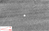 |
Fig. 1 Region of the sky adjacent to 288P. This deep image is the result of on-asteroid stacking of all the frames obtained with DEIMOS on Keck II and GMOS on Gemini South telescopes. North is up and east is to the left. On-sky projections of the prolonged radius vector and vector opposite to the orbital velocity vector (–V) are indicated. The dust tail, if present, should lie roughly between them. |
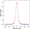 |
Fig. 2 Comparison of the cross sections of 288P profile (orange line connecting circles) and the typical stellar profile (blue line connecting squares). Both cross sections were normalised to 1.0 at the maximum signal and have a native CCD sampling. Each pixel had 0.118 arcsec during our observations. |
4 Photometric separation of the light curve
The light curve of 288P is presented in Fig. 3. It is quite densely sampled and reveals variability with a peak to peak amplitude close to 0.5 mag in R which can be attributed to the fact that the projection area of an elongated object changes due to rotation. Our data comprise almost one period of rotation if we take that the light curve is double peaked. Furthermore, our light curve looks like a combination of the two variabilities with quite different periods. Thanks to HST multi-epoch monitoring of this object during phases of undetectable activity it is established (Agarwal et al. 2020) that the brighter component (named A) changes its brightness in the range of 0.9 mag in F606W filter (central wavelength = 595.6 nm, and FWHM= 234.0 nm, Baggett et al. 2007) and the variability amplitude of the fainter component (called B) is close to 0.4 mag. As our light curve is a sum of the contributions coming from both fragments, the resultant amplitudes of long and short period variability are diminished with comparison to the HST results. Thus, our result appears to be consistent with previous findings. What is more, when 288P was inactive, the relatively stable amplitudes for both components were observed at quite different ecliptic longitudes close to 100, 113, 222 (Agarwal et al. 2020) and 245 degrees for our run. This can be achieved only if the rotation axes of both fragments are almost perpendicular to the ecliptic plane, which means that they are also almost perpendicular to the heliocentric orbit of the asteroid since its inclination to the ecliptic is 3.2°. Such case is consistent with the scenario in which the rotational splitting of the bilobate nucleus is responsible for the origin of the double asteroid. Its mutual orbit should be more or less perpendicular to the rotation axis of the parent body. The situation in which the rotation axis of the progenitor asteroid is co-aligned with the orbital angular momentum vector is statistically highly favoured due to the evolution of the rotation axis obliquity driven by the YORP mechanism (Hanuš et al. 2011; Cibulková et al. 2016).
To properly separate both components of 288P in photometric sense (that is to obtain both light curves, one for each component), we need information about the ratio of their mean fluxes or, equivalently, the difference between their mean magnitudes. We took this difference from Agarwal et al. (2020), where the lower and higher absolute magnitudes for both fragments are given as 17.1–18.0 and 17.9–18.3 mag in the ST F606W filter. Here we assumed that both components have identical spectral reflectance which means that the magnitude difference between both objects is independent of the photometric band used. We carried out the separation of the light curve into two components by an iterative procedure, determining the sidereal rotation periods, sizes, and shape parameters of both fragments in every step. To obtain the synthetic light curve, we used Hapke’s reflectance model (Hapke 2012) with a shadow-hiding opposition effect and macroscopic roughness influencing the reflectance properties. The details and model parameters were the same as we used previously (Drahus et al. 2018) analysing the light curve of ‘Oumuamua where we assumed that it is a C-class asteroid. 288P is also of the same type, as revealed by colourimetric observations (Licandro et al. 2013).
As a reasonable assumption, we took both fragments to be prolate two-axial ellipsoids, and later checked how this assumption affected our results. The first step of our procedure was to fit the model of a single elongated body to the total light curve. We accepted the reduced χ2 statistic as the parameter to be minimised to find the optimal solution. After the model was fitted we computed the differences between the observed and synthetic curves. Having this differential light curve, we carried out a periodicity analysis to look for frequencies other than the fundamental frequency of the modulation. Here we used the phase dispersion minimisation (PDM) method (Stellingwerf 1978) that is adequate for non-sinusoidal signal variations unevenly sampled in time. Because the original approach is insensitive to errors of the data points, we preferred our established version of PDM which offers an inverse-variance weighting of the input light curve (Drahus & Waniak 2006). The modified version, as the original algorithm, has two parameters that can be tuned according to the time series sampling and signal quality, which are number of bins Nb and number of covers Nc (Stellingwerf 1978). Figure 4 presents the resultant periodogram as the frequency dependence of the θ parameter for Nb = Nc = 12 which appeared to give the optimal result. To compute this parameter the data points are phased according to a given frequency and binned into Nb slots. For each bin the variance is computed and the mean variance for all the bins is obtained. At the end the result is normalised by dividing it by the variance of the unbinned data. This plot shows one global minimum at frequency 14.24 d−1 (time period of 3.37 h for a two-peaked light curve) accompanied by a series of period multiples. The triple structure of the negative peaks is the result of our specific time coverage of the light curve that can be identified with the spectral window characteristic of methods based on the Fourier transform. No peaks are visible at other frequencies, therefore we could be sure of the assumption that there are two distinct periodicities, each produced by one fragment of 288P.
In the next step of our separation procedure, the differential light curve was converted to the light curve of the second body using the magnitude difference between fragments. The separation of the photometric error into two components, each corresponding to the light curve of a given fragment, was made under the assumption that the Poisson noise is a predominant source of photometric uncertainty. The last assumption is consistent with the fact that our photometry was made in the regime of bright object – faint background. The next step was to synthesise the best fitted model light curve of component B searching for its size, semi-axis ratio, and rotation period via minimisation of the χ2 statistic. We then subtracted this model curve from the complete observational data to obtain the individual light curve of fragment A and this curve was used to search for the size, axis ratio, and rotation period of this component. For consecutive steps of our procedure, we checked whether the sum of both individual curves was identical to the total input light curve and whether the difference of the mean magnitudes of both components was equal to the assumed value.
Before using our method to analyse real data we checked its behaviour for a light curve, being the sum of synthetic curves produced by our reflectance model for a binary asteroid composed of two prolate spheroids. Preparing the test data, we tried to reproduce the observed total light curve of 288P. Our procedure converged to a stable solution very quickly. After two to three iterations, the discrepancies between the consecutive separated light curves (output of our procedure) appeared to be of the order of mmag. What is more the assumed input parameters (rotation periods, semi-axis ratios, sizes) and their output values were close enough to each other, and their proximity was fully controlled by the level of noise, which was incorporated into the input test light curve.
We realise that, on one hand, the component sizes obtained from the model approach depend substantially on the assumed geometric albedo, and on the other hand, the b/a semi-axis ratios (c axis is parallel to the object rotation axis) of both ellipsoids correlate with the accepted value of the magnitude difference between components. Hence we wanted to check how much our model approach is biased by uncertainty in our knowledge of geometric albedo or relative brightness of fragments A and B. Additionally we should free ourselves from the assumption that asteroid’s components are two-axial ellipsoids. In our case it is impossible to find two semi-axis ratios (b/a, c/a) simultaneously for each ellipsoid, but we can remove the assumption that b/a = c/a and try to separate the light curve for any reasonable c/a ratio. The last, but not least, question is whether the rotation of the fragments is in the same direction as the revolution of the mutual orbit. This issue is fundamental for the analysis of angular momentum. All the results presented going forwards were obtained under the assumption that the direction of rotation and revolution agree, but we also made the appropriate test with retrograde rotation of both fragments and obtained almost exactly the same results as for prograde rotation. This means that, based on our data, we are not able to distinguish the direction of rotation.
Having all this in mind we performed the separation procedure for three values of geometric albedo in the R photometric band (AR = 0.05, 0.07 and 0.10), two additional values of the difference between mean magnitudes of the components (0.2 mag lower and 0.2 mag higher than the nominal value), as well as for a c/a semi-axis ratio equal to 0.3, that is a substantially flattened triaxial ellipsoid. This ratio is about two times smaller than the b/a ratio inferred from our initial computations where we assumed prolate spheroids for both components.
Table 2 presents the results of separation of the light curve for all variants discussed above. We show the rotation periods, b/a ratios and semi-axes for fragments A and B. Although it may seem that presenting both semi-axis ratios and semi-axes themselves is redundant, the former were determined directly from the model analysis, while the latter were obtained from these ratios and the projection areas of the components.
Figure 5 shows the phased observational light curves together with the model generated light curves separately for both components. To properly match the light curves in phased plots, which is difficult because of the phase angle effect changing over time, we computed the model curves for the constant illumination and viewing geometry at the moment of the first data point. Photometric measurements were also adjusted to this specific geometry through corrections provided by our reflectance model, which takes this phase effect into account. We obtained the model light curves for components A and B once for the actual geometry changing over time, and once for the constant geometry. The magnitude differences between the photometric points of both curves were the phase effect corrections to be found.
Different variants of the model analysis of the light curve of 288P gave different geometric parameters (see Table 2) but provided us with almost the same reduced χ2 statistics equal to 1.46 indicating a fairly good agreement between the model curve and photometric data. As expected, the parameters that appear to be less dependent on the model variant and are almost constant (taking their errors into consideration) are both rotation periods. Hence, they can be considered as the most reliable results of our analysis. Different AR did not cause any significant change of the shapes of the components, keeping almost the same semi-axis ratios. On the other hand, the semi-axes themselves are dependent on the albedo. Interestingly, the sizes of both components for any albedo can be simply obtained by rescaling the results determined for a given albedo, at least for a small range of differences in AR. As can be seen in Table 2, the more complicated case occurs when the original magnitude difference between the mean brightness of A and B (taken from Agarwal et al. 2020) was changed to mimic a 0.1 mag uncertainty in the luminosity of each component. When this difference is reduced by 0.2 mag (A fainter, and B brighter than originally assumed), the semi-axis ratio for A diminishes (A becomes more elongated) and its size decreases, while for B the semi-axis ratio increases (B becomes less elongated) and the dimensions grow. The opposite situation occurs when the magnitude difference is increased by 0.2 mag. In the last variant of our model approach, where we assumed that the brighter component A is a triaxial ellipsoid with a c/a ratio equal to 0.3, we had to do with a slab rotating with respect to the axis of maximum inertia. For this rather unusual but not impossible situation (for example the Kuiper Belt object Arrokoth, McKinnon et al. 2020) we were provided with almost the same results (rotation periods, b/a ratios) as for A being a prolate spheroid. This outcome indicates that we can only put an upper limit on the c/a ratio, which should be less than b/a to ensure the unexcited rotation of object A. Whereas our data do not allow us to exclude excited rotation in this case, the very good match of the phased light curve for component B proves not excited rotation. Since we are only able to provide an upper limit for c semi-axes, it is difficult to perform a proper account of the angular momentum and energy. The same is true for both objects, but the parameters of B are less important for the binary system, as it is the less massive component.
Our semi-axes for AR = 0.07 remain in general agreement with the component sizes presented by Agarwal et al. (2020). One should remember that our photometry was carried out in the R band, whereas their observations were made with the HST F606W filter. However, our b/a ratios of the semi-axes are systematically greater by about 0.2 than their results, which may indicate that the rotation axes of both components are not perpendicular to the ecliptic plane. As the inclination of the heliocentric orbit of 288P is 3.2 deg, this can mean that the rotation axes are not perpendicular to the plane of the mutual orbit that is roughly parallel to the heliocentric orbit (Agarwal et al. 2020). Conversely, if the rotation axes are perpendicular to the mutual orbit, this orbit is not parallel to the heliocentric orbit. Certainly, both possibilities may be right. Anyway, this means that our b/a semi-axis ratios should be treated as upper limits.
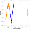 |
Fig. 3 Light curve of 288P. The data obtained by Gemini South GMOS are shown by orange circles and by Keck II DEIMOS by blue circles. The R magnitude is for 1.0 AU heliocentric and geocentric distances but was not corrected for the phase angle effect (explanation is given in the text). The UT date presents the moment of time retarded to the object’s position and given in fractions of a day starting from 0:0 UT on 21 May 2015. |
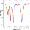 |
Fig. 4 Result of the periodicity search in the differential light curve obtained by subtracting the model curve for a slowly rotating pro-late spheroid from the original photometric data (for details see text). The orange line shows the result for all the data, whereas the blue line presents the result for the first compact run of the observations. |
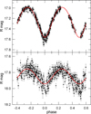 |
Fig. 5 Result of separation of the light curve into two components produced by the slowly (top panel) and rapidly (bottom panel) rotating fragments of 288P, respectively. The best fitted model curves (red lines) computed for the first case in Table 2 are also presented. Both curves were phased according to the appropriate sidereal periods. |
Parameters of the 288P components obtained for the different variants of light curve fitting.
5 The third component of 288P
The last question concerning the light curve of 288P is whether we observed the superposition of the signals produced by two components or we have to do with a larger number of bodies, each of them giving a periodic signal. As shown by Kim et al. (2020), the light curve of component A registered by HST is most probably the sum of long period (16 h) and short period (3.2 h) variability. Although we checked the differential light curve obtained by subtracting the model curve of a slowly rotating prolate spheroid from the photometric points and found only one distinct short period variability, this does not mean that this differential curve could not be the sum of two periodic signals with frequencies close to each other. As a result, the beat effect would be created and, for similar amplitudes of both components, we would observe periodic variability with a frequency equal to the mean frequency of both signals and with an amplitude modulated by a frequency that is half of the frequency difference. Such a situation is difficult to recognise using the PDM search, as the period of amplitude modulation may be much longer than the time duration of our observing run. In addition, our period 3.37 h (see Table 2) obtained for B is suspiciously close to the harmonic mean of the periods 3.2 h and 3.6 h, the first of which is the rotation period of component C constituting a close binary with larger, slowly rotating fragment A, and the second is the rotation period of B revolving around this tight pair (Kim et al. 2020). Components A and B are easily resolved in HST data, but fragments A and C would remain unresolved and produce the common light curve with long- and short-period variability.
Hence, we wanted to check if our results agree with the scenario of 288P being a triple, that is if our short period variability could be the beat effect produced by the superposition of the light curves for B and C. Because the amplitude of modulation is dependent on the ratio of the amplitudes of both components, we analysed different cases of such ratios for the situation where component B has a larger amplitude of variability than fragment C and vice versa. The first possibility is much more likely, as the individually determined amplitude for B (Agarwal et al. 2020) is even larger than our value. On the other hand, the too small amplitude for C could be associated with difficulties in detecting its brightness variation against the background of the common light curve with A. We chose a number of amplitude ratios from 1 to 1/4. For each ratio we determined the space of possible parameters, namely the semi-axis ratios for all three components (assuming that they were prolate spheroids) as well as the ratio of the maximum projection areas of components C and B. The contribution of B to the overall brightness of 288P is well known (Agarwal et al. 2020) and was previously used by us for separation of the light curve. Knowledge of the amplitudes of long- and short-period variability, provided by our data, made it possible to find this space of possible parameters. It turned out that, for each amplitude ratio for components B and C, this space included quite reasonable values of the parameters, with all three semi-axis ratios not lower than 0.3 and with sizes of the components being comparable to each other. This indicates that, in general, the scenario of triple 288P is plausible. However, the total volume of the three components having parameters selected from the appropriate spaces was always smaller than for a binary configuration, though by no more than 30%. This means a higher mean density of the object as obtained from its mass computed from the orbital period and its volume determined from the overall brightness. Taking into account the general uncertainties of this analysis, the effect is not significant.
We synthesised a light curve, that was the sum of 3.2 h and 3.6 h variability, with appropriate amplitude ratio giving a result as close to the observed differential light curve as possible (in the LSQ sense). This differential light curve was determined by subtracting from our data points the model curve for a single slowly rotating prolate spheroid. This was the first step in our procedure of light curve separation and has already been described. Contrary to our original approach, in which we used Hapke’s reflectance theory, here we accepted the sinusoidal variability as a quite good representation of a prolate spheroid. This way is much less time consuming and is fully acceptable taking into account both the small amplitude of the observed short-period brightness variability and the low S/N. In addition, our aim was not to find the physical parameters of the components, but only to represent their brightness variations. Unfortunately, the time coverage of our data points is not long enough to trace the whole period of amplitude modulation. In our case this period, being half of the harmonic difference between 3.2 and 3.6 h, is equal to about 58 h.
Thus, we computed the common light curve for different phases of modulation. This means that for our time points we had different and evenly distributed positions of maxima and minima of the amplitude modulation. The theoretical light curve was supplemented by the observational noise due to adding to each signal the difference between the observed noisy curve and the smooth, synthetic curve for our best model of double 288P. We then carried out the PDM periodicity analysis with the same parameters (Nb, Nc numbers and the same periodogram sampling) as previously. We compared the obtained results with the band periodogram representing the +/− 3σ region of possible values of θ parameter for the PDM analysis of the differential light curve (see previous section). This region was determined by the classic bootstrap approach.
Figure 6 shows the results of this comparison for 1.0 and 0.5 amplitude ratios of 3.2 and 3.6-h variability and for modulation phases giving the best and the worst PDM results as related to the band periodogram. Generally, we cannot definitively disprove the triplicity of 288P, but we obtained an acceptable PDM phasing only for amplitude ratios between 1 and 2/3 and only for some regions of the modulation phases not exceeding 10% of the whole range from zero to one. This ambiguity is a consequence of our specific temporal coverage of the light curve and the insufficiently high S/N of our data. With increasing disproportion between the amplitudes of both components the beat modulation is weaker and we observed double minima of the periodogram (at the frequency of dominating variability and at the mean of both component frequencies), or minima at the dominating frequency. We conclude that, except for restricted regions of the whole space of possible parameters, the beat effect produced by variability of B and C components of a triple asteroid should be quite easily detected in our data. Therefore, we treat the claim about existence of the third body in the double 288P with great caution.
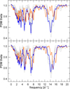 |
Fig. 6 Result of the PDM periodicity search for the test light curves. These curves are the superpositions of variability with a period of 3.6 h for B and 3.2 h for C, and for the ratio of the amplitude of B variability to the amplitude of C variability equal to 1.0 (top panel) and 0.5 (bottom panel), respectively. These periodograms are compared with the bound periodogram (grey lines) that is represented by the mean and the +/− 3σ limits in the case of our observations (for details see the text). The blue and orange lines are for phasing of the composite light curves that gives the best and worst compatibility between the observed and the test periodograms. |
6 Discussion
When we have quite precise values of the rotation periods, as well as the most probable shapes and sizes of both components of 288P, we can analyse the plausible evolutionary track of this binary active asteroid. Agarwal et al. (2017) and Agarwal et al. (2020) examine different scenarios involving its origin and evolution, pointing out that sublimative activity could play a major role. Here we focus on the evolution of the mutual orbit and the rotation state of the fragments after their disconnection. Generally, there are two approaches to this issue. The first one uses numerical simulations of the orbital and rotational motion with tidal interaction between components taken into account (e.g. Jacobson & Scheeres 2011). In the second method the total angular momentum and energy balances at different stages of evolution are analysed (e.g. Pravec & Harris 2007; Pravec et al. 2010).
We followed the latter approach and compared these quantities at the moment of fission with the actually observed values. The aim was to estimate how much angular momentum and energy was entered into the system as a result of the activity of the smaller component B. We assumed that rotational fission is responsible for separation of the two lobes of the parent body (arguments for that can be found in Section 4). We approximated the progenitor by a pair of the same ellipsoids representing components A and B as we obtained from our model separation of the light curve of 288P, interconnected by a neck. Its contribution to the gravitational attraction of the lobes was neglected. The mutual orientation of the merged ellipsoids could be arbitrary but ensuring the unexcited rotation of the whole body about the axis of maximal moment of inertia. The most plausible situation is when their shortest axes were parallel to each other and to the rotation axis of the whole body. Additionally, the line section connecting the mass centres of the lobes was perpendicular to this axis. We analysed four characteristic configurations of the lobe coupling (see Fig. 7) where they connect: top A to top B (denoted as TA−TB), top A to side B (TA − SB), side A to top B (SA−TB) and side A by side B (SA − SB). An example of the first kind of merging could be the contact binary nucleus of comet 8P (Harmon et al. 2010) whereas the last configuration is well represented by the nucleus of comet 67P (Massironi et al. 2015).
For each configuration we arbitrarily, but reasonably, assumed that the area of the neck cross section (line n–n in Fig. 7) makes up one quarter of the smaller of the maximum cross sections for both lobes, cross sections perpendicular to the line connecting mass centres (lines a–a and b–b in Fig. 7). The first step was estimation of the critical rotation period when the centrifugal force overcomes gravity and the cohesive force, causing a crack of the bilobate nucleus in the neck region (Hirabayashi et al. 2016). We followed here the simple approach presented by Hui et al. (2023); however, we did not approximate components by spheres but numerically computed the gravitational attraction between ellipsoidal lobes. Although knowledge of the cohesion strength for different classes of small solar system bodies is poor, there are many estimations of this quantity indicating that it is in the tens or single hundreds of Pa (Davidsson 2001; Rozitis et al. 2014; Hirabayashi et al. 2014, 2016). Here we took the range from 0 to the value for which the orbital energy after fission becomes positive. Certainly, just before reaching this point, the mutual distance between components appears greater than the Hill radius (of order 300 km). The densities, identical for both lobes, were computed from the total mass of the components. This is estimated by Agarwal et al. (2020) from Kepler’s third law and appears to be in the range of (6.67–7.23)×1012 kg. Taking the average value of the mass, we obtained densities from about 1300 kg m−3 for geometric albedo 0.05, through 2200 kg m−3 for albedo 0.07, to 3800 kg m−3 for albedo 0.10. Only first two quantities seem to be reliable for a C-class asteroid. The remaining cases from Table 2 gave densities from 1600 to 2200 kg m−3. The dependence of the critical rotation period on the ratio of cohesive to gravity force Fc/Fg is presented in the upper panel of Fig. 8.
We show the results for cases 1, 2, 3, and 6 from Table 2. Two other cases gave values close to the first variant with an albedo of 0.07. For better readability, we only present dependencies for configurations TA–TB and SA–SB which provided us with extreme results. As expected, the more compact object (SA − SB merger) splits at a shorter rotation period. For convenience, we mark the positions where the cohesive force is equal to the product of the appropriate cross-sectional area of the neck and the cohesive strength equal to some characteristic values between 0 and 1000 Pa (see the caption of Fig. 8). This procedure allows for estimation of the cohesive to gravity force ratio for different values of cohesion strength and/or neck cross-sectional area. The overwhelming majority of the critical rotation periods appeared to be between the actual rotation periods of A and B. Only one case of the most compact initial configuration SA − SB and the highest albedo of 0.1 (case 3 from Table 2) provides us with a critical rotation period that is shorter than the recent period for B, but this variant is related to the suspiciously high density of 3800 kg m−3.
Numerical simulations by Jacobson & Scheeres (2011) show that the maximal separation between components that can be achieved after 100 years of evolution starting from the rotational splitting is markedly dependent on their mass ratio. For all cases analysed by us, the mass ratio was between 0.28 variant 6 in Table 2) and 0.54 (case 4). For such mass ratios, the maximum separation is less than ten sizes of the primary. To answer the question of how much total angular momentum and free energy (Pravec et al. 2010) were entered into the system during its evolution to enlarge the mean separation to almost 100 primary sizes, we compared the above quantities at the moment of fission with today’s values. We computed the recent orbital energy and angular momentum using the mean values of the orbital parameters given by Agarwal et al. (2020). Although the eccentricity was obtained with a relatively large uncertainty of 10% (from 0.41 to 0.51), the factor  appearing in the angular momentum formula has a range from 0.86 to 0.91, which means that the divergence is less than 3%. The central panel of Fig. 8 presents the relative change in total angular momentum, whereas the bottom panel shows the relative change in free energy, both as functions of the ratio Fc/Fg and related to the current values. Because recently over 90% of total angular momentum falls on the orbital motion, the relative gain of the total quantity should not depend much on the initial state of the system and Fig. 8 confirms this. For different variants analysed by us and for reliable cohesive strength the relative increase is between 60% and 80%. Although this surplus was estimated assuming recent prograde rotation for both fragments, we also analysed the situation where component B rotates in the retrograde direction. This is consistent with our scenario of orbit evolution that will be presented later in this section. The differences between both estimates were smaller than 2% and we remind the reader that we were unable to determine the direction of rotation. Counting the balance of free energy, we did not take into consideration the work of the cohesive force in lobe separation because cohesion is a very short-range interaction and therefore is rather negligible compared to the gravitational energy of the system if both forces are of the same order. Figure 8 indicates that in the case of an increase in free energy the situation is more complicated than for total angular momentum. The reason is that currently only a few percent is contained in orbital energy and even negative relative gains are possible for higher cohesive strengths. In such a situation, energy dissipated by the tidal interactions overcomes kinetic energy entered into the system.
Only two known mechanisms, apart from collision, which is rather unlikely, can deliver angular momentum and energy from outside. These are radiative BYORP or its sublimation-driven version in which the sublimative torque affects a tidally locked binary much more than radiation. For the sake of simplicity and consistency we dare to name it SBYORP. Generally, SBYORP is much more efficient than BYORP just like sublimative YORP (SYORP) is a couple of orders more effective than radiative YORP (Steckloff & Jacobson 2016). Hence, SBYORP was proposed as the dominant mechanism driving orbit evolution in 288P (Agarwal et al. 2017). Both, radiative and sublimative, YORPs require synchronisation of rotation with mutual orbital motion (tidal locking). At present the B fragment of 288P, suspected of activity, is very far from tidal locking. It is possible to estimate the time constant of its synchronisation (e.g. Gladman et al. 1997; Paele 1977) but this needs values of the tidal Love number k2 and the quality factor Q, which are both poorly known. Furthermore, the result is proportional to the sixth power of the mean distance between the components, which evolves over time. Instead we can calculate the ratio of the synchronisation timescale for B to the time it takes to slow down the rotation of A from the critical period to today value. This result is not dependent on poorly known parameters. We found ratios from 0.05 (case 6 in Table 2) to 0.35 (variant 4), which means that fragment B should be tidally locked for a long time. If the components of a binary asteroid are not active, its evolution can produce a wide asynchronous binary due to appropriate cooperation between the tidal interaction, radiative YORP and BYORP (Jacobson et al. 2014). When the smaller fragment, which is easier to tidally slow down, is active, the sublimative torque could obstruct or make impossible tidal locking unless its activity was triggered by a collision that took place after synchronisation, which while not impossible is rather unlikely for 288P.
Here we propose a self-consistent scenario based entirely on the activity of the smaller fragment B. Its sublimative torque may not only not counteract the tidal torque but may support or even replace it by being more effective. This is understandable because the tidal interaction decreases inversely proportionally to the sixth power of the mean mutual distance between fragments and the sublimation driven spinning up does not. After locking by SYORP, the sublimation driven BYORP can work. The only requirement is that the timescale of synchronisation is markedly longer than the timescale for effective angular momentum and energy pumping by SBYORP. To check this possibility, we first computed the timescale of SYORP τSYORP expressed by the number of perihelion passages of 288P it takes to slow down the rotation of B from the initial critical rate to synchronisation and then spin up to the actual rotation rate, assuming that each perihelion passage causes activity similar to that observed in 2000 and 2016 (Hsieh et al. 2018). Based on their results we used the production rate of dust equal to 4.55 kg s−1 and duration of activity of 195 days, as averages of two periods. We assumed that 288P was active for the same length of time pre-and post-perihelion and that there is one active region on B, which is consistent with the assertion that only a tiny fragment (at most a few percent) of the whole surface was active in 2000 and 2016 (Hsieh et al. 2018). This kind of activity, where the active region is periodically illuminated and periodically ejects matter, should produce arc structures in the dust coma. Unfortunately because of the very small dust ejection velocity of the order of 1 m s−1 (Hsieh et al. 2018) and relatively fast rotation they may be undetectable.
We conservatively took the dust to gas mass ratio as equal to 10 (Fulle et al. 2016), although values between 10 and 30 were reported by Reach et al. (2000). We pessimistically assumed that gas emission was isotropic in half of the full solid angle (degree of jet collimation equal to 0.5) that lowered the effective recoil force by a factor of two. The gas ejection velocity was the same as in Agarwal et al. (2020) and equaled 500 m s−1. The least well known parameter is the effective arm of the recoil force, which is dependent on the general shape and macroscopic structure of the body’s surface. We computed the mean value of this arm for B for our different cases assuming that the active region can be placed at random position on the ellipsoidal object with a constant surface PDF, but only on the appropriate portion of the body to slow down rotation and not produce noticeable torque causing excited rotation. The last condition means that the region is located near the equatorial plane perpendicular to the rotation axis. For smooth surface of the ellipsoid we calculated the angle between the local normal to the surface and the radial vector attached in the mass centre. The ratio of the effective arm to the longest semi-axis a, which correlates with the degree of spheroid elongation, may change from 0 to a maximum value that appeared to be from 0.120 for case 5 to 0.145 for case 1 in Table 2. We used the Monte Carlo approach to determine the mean effective arm. This arm divided by the longest semi-axis turned out to be between 0.077 for variant 5 and 0.094 for variant 1, respectively. Eventually we obtained the numbers from 1500 to 3900 orbital periods for different cases from Table 2, different mutual orientations of the merged lobes before splitting (from TA−TB to SA−SB) and cohesion strength of the order of 200 Pa. This represents 2700 perihelion passages on average, that is about 14 000 years and can be confronted with the timescale of double synchronisation of the system, which is close to 50 000 years for this mass ratio (Jacobson & Scheeres 2011).
In a similar way, we computed the timescale of SBYORP τS BYORP expressed in the number of perihelion passages of 288P required to increase the total angular momentum to the currently observed value, assuming that the component presenting sublimative activity is synchronised all the time and SBYORP can work. We did not analyse here the energy balance because energy is dissipated via the tidal interactions. To transfer the recoil force produced by gas emission into the orbital torque we need the value of the effective arm of this force. We arbitrarily took it as equal to half the actual semi-major axis obtained by Agarwal et al. (2020). This is supposed to approximate the average of the semi-major axis at the moment when SYORP synchronised fragment B, and the actual semi-major axis. We assumed, just as previously when computing the effective arm of the rotational torque, that the active region is arbitrarily located near the equatorial plane perpendicular to the rotation axis of B. This is consistent with the requirement that the sublimative non-gravitational acceleration has a negligible normal component which could change the orientation of the mutual orbital plane. We obtained 2/π as the mean sine of the angle between the orbital radius vector for a circular orbit and the recoil force changing the orbital angular momentum. Eventually we were provided with a number of perihelion passages between 70 and 120 for our different variants and cohesion strength of the order of 200 Pa. Agarwal et al. (2017) estimate the timescale of doubling the orbital angular momentum as about 900 perihelion passages, which is almost an order of magnitude larger than our evaluation, but both were made using different input parameters and both have an uncertainty of an order of magnitude.
Although our estimations of the SYORP and SBYORP timescales were based on uncertain assumptions and used many poorly known parameters, the ratio of both is much more reliable, being independent of the history of dust production (taking into account the effect of shadowing of B by A), dust to gas ratio, gas ejection velocity and degree of jet collimation. The ratio τSYORP/τSBYORP is presented in Table 3 for all cases from Table 2 and all variants of lobe coupling. This table contains ranges of this ratio where the first value indicates zero cohesion whereas the last value was computed for the ratio of Fc/Fg giving zero orbital energy after fission (like dependencies presented in Fig. 8). For all cases and variants, the timescale ratio increases monotonically and smoothly with Fc/Fg. For the cohesion strength equal to 200 Pa the ratio τSYORP/τS BYORP turned out to be from about 20 (cases 3 and 6 from Table 2) to 32 (case 4) which means that SBYORP might have had enough time to pump an appropriate amount of angular momentum and kinetic energy into 288P, enabling evolution of its orbit. Most probably this process took place in a number of stages. After initial synchronisation by SYORP at a given orbital period, SBYORP gains angular momentum and energy causing the semi-major axis to increase and the orbital period to get longer, inducing desynchronisation and a decrease in SBYORP efficiency. After consecutive synchronisation of B by SYORP at the next stage, SBYORP can work again, and so on until B starts rotating in the opposite direction. A situation where one and the same active region is responsible for both spinning up the bilobate asteroid to the point of fission, and then decreasing rotation rate of the B lobe on which it is located, is not impossible and is quite likely for TA– TB and SA–TB lobe mergers, when the active region is located on the hemi-lobe whose pole is situated at the neck connecting both components before splitting. Such a region could have been created by excavation of a fresh icy layer by collisional disruption (e.g. Jewitt et al. 2015).
Agarwal et al. (2020) suggest that after perihelion passage in 2016 there was a change in the orbital parameters, which they attribute to sublimative activity. They compared this observed evolution with the change that could be provided by gas emission connected with dust production reported by Hsieh et al. (2018). The result shows that only tiny fraction of the possible change was realised. This is not unusual, as the B component is not synchronised and the change of orbit was caused only by the residual sublimative effect resulting from the random arrangement of the location of the active region and positions in the mutual and heliocentric orbits. Such an effect can produce only small, chaotic change of the orbital parameters. Certainly, spinning up of 288P B by SYORP could be detectable but we estimated that after one activity episode near perihelion the expected change of the rotation period is more than ten times smaller than our precision of period determination (see Table 2).
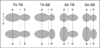 |
Fig. 7 Schematic view of the different configurations of the lobe coupling in the parent 288P. The top and bottom rows present views from directions perpendicular and parallel to the rotation axis, respectively. The elongation of the smaller component B is excessively increased for clarity. Lines a–a and b–b show the maximum cross sections of the lobes A and B in the direction perpendicular to the line that connects their mass centres. Line n–n indicates the cross section of the neck. |
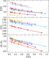 |
Fig. 8 Dependence of the critical rotation period Pc (top panel), relative increase in total angular momentum ∆L/L (middle panel), and free energy ∆Ef /Ef (bottom panel) on the ratio of the cohesive force Fc to gravity force Fg. Both gains are related to the current values of the quantities. The lines end at the ratio value for which the orbital energy of the system becomes positive after fission. The violet, blue, and yellow lines indicate AR equal to 0.07, 0.05, and 0.10 (cases 1, 2, and 3 in Table 2) whereas the red line is for case 6. Diamonds show the initial lobe configuration TA − TB and squares mean SA − SB merger. Symbols are placed where values of the cohesive to gravity force ratio correspond to the cohesive strength of 50, 100, 200, 400, 700, and 1000 Pa for the assumed value of the neck cross-sectional area. |
7 Conclusions
We made photometric observations of 228P near the aphelion of its orbit, between 21 and 22 May 2015 using the DEIMOS and GMOS instruments on the Keck II and Gemini South telescopes, respectively. We analysed 444 images as well as the light curve received from them. Our main results can be concluded as follows:
The deep image of the sky region that neighbours the asteroid and has about 3 square arcmin reveals no companion fragments larger than about 160 m in diameter;
The asteroid was almost completely inactive during our run, with a dust production rate on the order of at most tens of grams per second, which is 100 times lower than the typical near-perihelion rate (Hsieh et al. 2018). This trace activity only slightly disturbs the object’s light curve;
Using Hapke’s reflectance theory and the average brightness ratio of the A and B components from Agarwal et al. (2020), we separated the composite light curve and obtained one curve for each fragment. When we approximated A and B by prolate spheroids, we determined sidereal rotation periods of 15.86 and 3.37 hours and semi-axes equal to 1.12, 0.69 and 0.67, 0.57 km for the larger and smaller component, if we take an albedo in the R band of 0.07. This is in general agreement with the earlier estimation by Agarwal et al. (2020);
Our data cannot definitely confirm or contradict the existence of a third body accompanying fragment A (Kim et al. 2020), however, we find this possibility unlikely;
An analysis of the recent content of total angular momentum and free energy in 288P compared to the state at the moment of rotational fission of the bilobate progenitor indicates that the gain of both quantities was caused by sublimative activity of the smaller component. This is plausible given that, most probably, the timescale of its SYORP synchronisation is much longer than the timescale of SBYORP-induced increase in angular momentum from the initial to recent value. We consider rotational disconnection as a highly probable mechanism of fission, resulting from sublimative torque rather than from radiative YORP.
Data availability
Table 4 containing our light curve of 288P is available at the CDS via https://cdsarc.cds.unistra.fr/viz-bin/cat/J/A+A/704/A169.
Acknowledgements
Based on observations obtained at the international Gemini Observatory, a program of NSF NOIRLab, which is managed by the Association of Universities for Research in Astronomy (AURA) under a cooperative agreement with the U.S. National Science Foundation on behalf of the Gemini Observatory partnership: the U.S. National Science Foundation (United States), National Research Council (Canada), Agencia Nacional de Investigación y Desarrollo (Chile), Ministerio de Ciencia, Tecnología e Innovación (Argentina), Ministério da Ciência, Tecnologia, Inovações e Comunicações (Brazil), and Korea Astronomy and Space Science Institute (Republic of Korea). Some of the data presented herein were obtained at Keck Observatory, which is a private 501(c)3 non-profit organization operated as a scientific partnership among the California Institute of Technology, the University of California, and the National Aeronautics and Space Administration. The Observatory was made possible by the generous financial support of the W. M. Keck Foundation. M.D. is grateful for support from the National Science Centre of Poland through FUGA Fellowship grant 2014/12/S/ST9/00426 and SONATA BIS grant 2016/22/E/ ST9/00109. The authors gratefully acknowledge an anonymous referee for very useful and constructive comments.
References
- Agarwal, J., Jewitt, D., Weaver, H., Mutchler, M., & Larson, S. 2016, AJ, 151, 12 [Google Scholar]
- Agarwal, J., Jewitt, Mutchler, M., Weaver, H., & Larson, S. 2017, Nature, 549, 357 [Google Scholar]
- Agarwal, J., Kim, Y., Jewitt, D., et al. 2020, A&A, 643, A152 [EDP Sciences] [Google Scholar]
- A’Hearn, M. F., Schleicher, G. D., Feldman, P. D., Millis, R. L., & Thompson, D. T. 1984, AJ, 89, 579 [CrossRef] [Google Scholar]
- Baggett, S., Boucarut, R., Telfer, R., Quijano, J. K., & Quijada, M. 2007, Performance of the WFC3 Replacement UVIS Filters, Tech. rep. [Google Scholar]
- Bessell, M. S. 1979, PASP, 91, 589 [Google Scholar]
- Bottke, W. F., Nolan, M. C., Greenberg, R., & Kolvoord, R. A. 1994, Icarus, 107, 255 [NASA ADS] [CrossRef] [Google Scholar]
- Buchhaim, B. 2005, SASS, 24, 111 [Google Scholar]
- Cibulková, H., Ďurech, J., Vokrouhlický, D., Kaasalainen, M., & Oszkiewicz, D. A. 2016, A&A, 596, A57 [NASA ADS] [CrossRef] [EDP Sciences] [Google Scholar]
- Ćuk, M., & Burns, J. A. 2005, Icarus, 176, 418 [Google Scholar]
- Davidsson, B. J. R. 2001, Icarus, 149, 375 [Google Scholar]
- Drahus, M., & Waniak, W. 2006, Icarus, 185, 544 [Google Scholar]
- Drahus, M., Waniak, W., Tendulkar S., et al. 2015, ApJ, 802, L8 [NASA ADS] [CrossRef] [Google Scholar]
- Drahus, M., Guzik, P., Waniak, W., et al. 2018, Nat. Astron., 2, 407 [NASA ADS] [CrossRef] [Google Scholar]
- Durda, D. D., Bottke, W. F., Enke, B. L., et al. 2004, Icarus, 167, 382 [NASA ADS] [CrossRef] [Google Scholar]
- Faber, S. M., Phillips, A. C., Kibrick, R. I., et al. 2003, Proc. SPIE, 4841, 1657 [NASA ADS] [CrossRef] [Google Scholar]
- Fink, U., & Rubin, M. 2012, Icarus, 221, 72 [Google Scholar]
- Fukugita, M., Ichikawa, T., Gunn, J. E., et al. 1996, AJ, 111, 1748 [Google Scholar]
- Fulle, M., Marzari, F., Della Corte, V., et al. 2016, ApJ, 821, 19 [NASA ADS] [CrossRef] [Google Scholar]
- Gimeno, G., Roth, K., Chiboucas, K., et al. 2016, Proc. SPIE, 9908, 99082 [Google Scholar]
- Gladman, B., Quinn, D. D., Nicholson, P., & Rand, R. 1997, Icarus, 122, 166 [Google Scholar]
- Hanuš, J., Ďurech, J., Brož, M., et al. 2011, A&A, 530, A134 [NASA ADS] [CrossRef] [EDP Sciences] [Google Scholar]
- Hapke, B. 2012, Theory of Reflectance and Emittance Spectroscopy (Cambridge: Cambridge University Press) [Google Scholar]
- Harmon, J. K., Nolan, M. C., Giorgini, J. D., & Howell, E. S. 2010, Icarus, 207, 499 [CrossRef] [Google Scholar]
- Hirabayashi, M., Scheeres, D. J., Sánchez, D. P., & Gabriel, T. 2014, ApJ, 789, L12 [NASA ADS] [CrossRef] [Google Scholar]
- Hirabayashi, M., Scheeres, D. J., Chesley, S. R., et al. 2016, Nature, 534, 352 [Google Scholar]
- Hook, I., Jørgensen, I., Allington-Smith, J. R., et al. 2004, PASP, 116, 425 [NASA ADS] [CrossRef] [Google Scholar]
- Hsieh, H. H., & Jewitt, D. 2006, Science, 312, 561 [NASA ADS] [CrossRef] [Google Scholar]
- Hsieh, H. H., Yang, B., Haghighipour, N., et al. 2012, ApJ, 748, L15 [NASA ADS] [CrossRef] [Google Scholar]
- Hsieh, H. H., Ishiguro, M., Kim, Y., et al. 2018, AJ, 156, 223 [NASA ADS] [CrossRef] [Google Scholar]
- Hui, M-T., Kelley, M. S. P., Hung, D., et al. 2023, AJ, 166, 47 [Google Scholar]
- Jacobson, S. A., & Scheeres, D. J. 2011, Icarus, 214, 161 [CrossRef] [Google Scholar]
- Jacobson, S. A., Scheeres, D. J., & McMahon, J. 2014, ApJ, 780, 60 [Google Scholar]
- Jewitt, D. 2012, AJ, 143, 66 [CrossRef] [Google Scholar]
- Jewitt, D., & Hsieh, H. H. 2024, in Comets III, ed. K. J. Meech (Tuscon: University of Arizona Press), 767 [Google Scholar]
- Jewitt, D., Li, J., Agarwal, J., et al. 2015, AJ, 150, 76 [Google Scholar]
- Kim, Y., Agarwal, J., & Jewitt, D. 2020, BAAS, 52, 6 [Google Scholar]
- Landolt, A. U. 1992, AJ, 104, 340 [Google Scholar]
- Licandro, J., Moreno, F., de León, J., et al. 2013, A&A, 550, A17 [NASA ADS] [CrossRef] [EDP Sciences] [Google Scholar]
- Massironi, M., Simioni, E., Marzari, F., et al. 2015, Nature, 526, 402 [NASA ADS] [CrossRef] [Google Scholar]
- McKinnon, W. B., Richardson, D. C., Marohnic, J. C., et al. 2020, Science, 367, eaay6620 [CrossRef] [Google Scholar]
- Novaković, B., Hsieh, H. H., & Cellino, A. 2012, MNRAS, 424, 1432 [Google Scholar]
- Paele, S. J. 1977, in Planetary Satellites, ed. J. A. Burns (Tucson: University of Arizona Press), 87 [Google Scholar]
- Pravec, P., & Harris, A. W. 2007, Icarus, 190, 250 [CrossRef] [Google Scholar]
- Pravec, P., Vokrouhlický, D., Polishook, D., et al. 2010, Nature, 466, 1085 [NASA ADS] [CrossRef] [Google Scholar]
- Reach, W. T., Sykes, M. V., Lien, D., & Davies, J. K. 2000, Icarus, 148, 80 [NASA ADS] [CrossRef] [Google Scholar]
- Rozitis, B., MacLennan, E., & Emery, J. P. 2014, Nature, 512, 174 [CrossRef] [Google Scholar]
- Rubincam, D. P. 2000, Icarus, 148, 2 [Google Scholar]
- Steckloff, J. K., & Jacobson, S. A. 2016, Icarus, 264, 160 [Google Scholar]
- Stellingwerf, R. F. 1978, ApJ, 224, 953 [Google Scholar]
- Stetson, P. B. 2000, PASP, 112, 925 [Google Scholar]
- Vokrouhlický, D., & Čapek, D. 2002, Icarus, 159, 449 [CrossRef] [Google Scholar]
- Vokrouhlický, D., Nesvorný, D., & Bottke, W. F. 2003, Nature, 425, 147 [Google Scholar]
- Walsh, K. J., Richardson, D. C., & Michel, P. 2008, Nature, 454, 188 [Google Scholar]
- Warner, B. D. 2006, A Practical Guide to Lightcurve Photometry and Analysis (Colorado Springs: Springer Science+Business Media, Inc.) [Google Scholar]
All Tables
Parameters of the 288P components obtained for the different variants of light curve fitting.
All Figures
|
Fig. 1 Region of the sky adjacent to 288P. This deep image is the result of on-asteroid stacking of all the frames obtained with DEIMOS on Keck II and GMOS on Gemini South telescopes. North is up and east is to the left. On-sky projections of the prolonged radius vector and vector opposite to the orbital velocity vector (–V) are indicated. The dust tail, if present, should lie roughly between them. |
| In the text | |
|
Fig. 2 Comparison of the cross sections of 288P profile (orange line connecting circles) and the typical stellar profile (blue line connecting squares). Both cross sections were normalised to 1.0 at the maximum signal and have a native CCD sampling. Each pixel had 0.118 arcsec during our observations. |
| In the text | |
|
Fig. 3 Light curve of 288P. The data obtained by Gemini South GMOS are shown by orange circles and by Keck II DEIMOS by blue circles. The R magnitude is for 1.0 AU heliocentric and geocentric distances but was not corrected for the phase angle effect (explanation is given in the text). The UT date presents the moment of time retarded to the object’s position and given in fractions of a day starting from 0:0 UT on 21 May 2015. |
| In the text | |
|
Fig. 4 Result of the periodicity search in the differential light curve obtained by subtracting the model curve for a slowly rotating pro-late spheroid from the original photometric data (for details see text). The orange line shows the result for all the data, whereas the blue line presents the result for the first compact run of the observations. |
| In the text | |
|
Fig. 5 Result of separation of the light curve into two components produced by the slowly (top panel) and rapidly (bottom panel) rotating fragments of 288P, respectively. The best fitted model curves (red lines) computed for the first case in Table 2 are also presented. Both curves were phased according to the appropriate sidereal periods. |
| In the text | |
|
Fig. 6 Result of the PDM periodicity search for the test light curves. These curves are the superpositions of variability with a period of 3.6 h for B and 3.2 h for C, and for the ratio of the amplitude of B variability to the amplitude of C variability equal to 1.0 (top panel) and 0.5 (bottom panel), respectively. These periodograms are compared with the bound periodogram (grey lines) that is represented by the mean and the +/− 3σ limits in the case of our observations (for details see the text). The blue and orange lines are for phasing of the composite light curves that gives the best and worst compatibility between the observed and the test periodograms. |
| In the text | |
|
Fig. 7 Schematic view of the different configurations of the lobe coupling in the parent 288P. The top and bottom rows present views from directions perpendicular and parallel to the rotation axis, respectively. The elongation of the smaller component B is excessively increased for clarity. Lines a–a and b–b show the maximum cross sections of the lobes A and B in the direction perpendicular to the line that connects their mass centres. Line n–n indicates the cross section of the neck. |
| In the text | |
|
Fig. 8 Dependence of the critical rotation period Pc (top panel), relative increase in total angular momentum ∆L/L (middle panel), and free energy ∆Ef /Ef (bottom panel) on the ratio of the cohesive force Fc to gravity force Fg. Both gains are related to the current values of the quantities. The lines end at the ratio value for which the orbital energy of the system becomes positive after fission. The violet, blue, and yellow lines indicate AR equal to 0.07, 0.05, and 0.10 (cases 1, 2, and 3 in Table 2) whereas the red line is for case 6. Diamonds show the initial lobe configuration TA − TB and squares mean SA − SB merger. Symbols are placed where values of the cohesive to gravity force ratio correspond to the cohesive strength of 50, 100, 200, 400, 700, and 1000 Pa for the assumed value of the neck cross-sectional area. |
| In the text | |
Current usage metrics show cumulative count of Article Views (full-text article views including HTML views, PDF and ePub downloads, according to the available data) and Abstracts Views on Vision4Press platform.
Data correspond to usage on the plateform after 2015. The current usage metrics is available 48-96 hours after online publication and is updated daily on week days.
Initial download of the metrics may take a while.