| Issue |
A&A
Volume 704, December 2025
|
|
|---|---|---|
| Article Number | A31 | |
| Number of page(s) | 21 | |
| Section | Interstellar and circumstellar matter | |
| DOI | https://doi.org/10.1051/0004-6361/202555994 | |
| Published online | 28 November 2025 | |
Probing sulphur chemistry in oxygen-rich asymptotic giant branch stars with ALMA
1
Rosseland Centre for Solar Physics, University of Oslo,
PO Box 1029
Blindern,
0315
Oslo,
Norway
2
Institute of Theoretical Astrophysics, University of Oslo,
PO Box 1029
Blindern,
0315
Oslo,
Norway
3
Dep. of Space, Earth and Environment, Chalmers University of Technology, Onsala Space Observatory,
43992
Onsala,
Sweden
4
School of Physics & Astronomy, Monash University,
Wellington Road,
Clayton
3800,
Victoria,
Australia
5
Institute of Astronomy, KU Leuven,
Celestijnenlaan 200D,
3001
Leuven,
Belgium
★ Corresponding author: This email address is being protected from spambots. You need JavaScript enabled to view it.
Received:
17
June
2025
Accepted:
6
October
2025
Abstract
Context. Sulphur and its isotopic ratios play a crucial role in our understanding of the physical properties of astrophysical environments; in particular, providing key insights into nucleosynthesis, interstellar medium processes, star formation, planetary system evolution, and galactic chemical evolution.
Aims. We aim to investigate the distribution of sulphur species - SO2, 34SO2, SO, and 34SO - towards a sample of five oxygen-rich asymptotic giant branch (AGB) stars, along with measurements of excitation temperature, column density, and isotopic ratios.
Methods. We used ALMA Band 6, 7, and 8 data of o Ceti, R Dor, W Hya, R Leo, and EP Aqr. SO2,34SO2, SO, and 34SO were detected towards AGB stars using the CASSIS software. To estimate the gas temperature and column density of these species, we applied the rotational diagram method (when applicable) and the Markov chain Monte Carlo method, assuming local thermodynamic equilibrium (LTE). Finally, line imaging of different transitions was performed to infer the distributions of the detected sulphur-bearing species in our sample.
Results. The measured excitation temperatures of SO2 for our sample sources range from ∼200 to 600 K, with estimated column densities in the range of 1-7 × 1016 cm−2. The excitation temperatures estimated using 34SO2 are comparable or slightly lower, while the column densities are about an order of magnitude lower than those of SO2. Our measured 32S/34S ratios for R Dor and W Hya are close to the solar value; however, the measured value for o Ceti is slightly higher, and the measured values for EP Aqr and R Leo are lower. Finally, spatial analysis shows that most detected lines appear as centralized emissions. Moreover, the high excitation transitions of SO2 show compact emission and probe hot gas of the inner region circumstellar envelopes (CSEs), whereas low-excitation transitions trace slightly extended structures. However, we find some differences in the emission of detected species across our sample.
Conclusions. The excitation temperature of the observed regions of the CSE can be probed using the SO2 molecule. The morphological correlation between SO and SO2 emissions suggests that they are chemically linked. Differences in the emission distributions of the detected species across our sample of low mass-loss rate AGB stars such as (i) centralized emission towards o Ceti with irregular emission shapes, (ii) centralized emission with ordered circular features towards R Leo and W Hya, (iii) clumpy emission features in R Dor, and (iv) unresolved emission in Ep Aqr may arise from several factors, i.e. the physical conditions of the sources (e.g. density and temperature structures of the CSEs), source multiplicity, outflows, rotation, or other associated physical processes such as thermal and nonthermal desorption, the effects of UV photons and cosmic rays, and finally the resolution of our observations. Nonetheless, the predominantly centralized distributions of SO and SO2 in our sample support previous findings for low mass-loss rate AGB stars. Our measured 32S/34S ratios for the two stars R Dor and W Hya agree well with solar values within uncertainties, indicating that these ratios likely reflect the isotopic composition of the stars’ natal clouds and deviate for three stars (o Ceti, R Leo, and EP Aqr), which could be due to the metallicity and/or excitation conditions within various sources.
Key words: astrochemistry / line: identification / instrumentation: interferometers / stars: abundances / stars: AGB and post-AGB / circumstellar matter
© The Authors 2025
 Open Access article, published by EDP Sciences, under the terms of the Creative Commons Attribution License (https://creativecommons.org/licenses/by/4.0), which permits unrestricted use, distribution, and reproduction in any medium, provided the original work is properly cited.
This article is published in open access under the Subscribe to Open model. This email address is being protected from spambots. You need JavaScript enabled to view it. to support open access publication.
1 Introduction
When a star with an initial mass of 1-8 M⊙ approaches the end of its life and enters the asymptotic giant branch (AGB) phase, during which it rapidly loses mass (in the range 10−8-10−4 M⊙ yr−1) and consequently creates an expanding circumstellar envelope (CSE). In the AGB phase, the star undergoes periodic events known as thermal pulses, which trigger dredge-up episodes that bring carbon from the interior to the surface. If the carbon abundance at the surface exceeds that of oxygen, the star transforms into a carbon star. Depending on the C/O ratio, an AGB star can be classified as oxygen-rich when C/O < 1, carbon-rich when C/O > 1, and S-type where C/O ~ 1.
Sulphur is the tenth most abundant element by mass in the Universe, and it plays a crucial role in biological systems (Mifsud et al. 2021; Krijt et al. 2023). Sulphur has four stable isotopes with fractional abundances of 32S (94.85%), 33S (0.76%), 34S (4.36%), and 36S (0.02%), reflecting their relative abundances at the time of the birth of the Sun (Asplund et al. 2021). The sulphur isotope ratio provides crucial and complementary information on stellar synthesis that is not traced by carbon (Yan et al. 2023). It is believed that 32S and 34S are mainly synthesized during the oxygen-burning process of Type II and Type Ia supernovae (SNe) and 33S synthesized in explosive oxygen and neon-burning (Woosley & Weaver 1995; Yan et al. 2023).
Asplund et al. (2021) report a ratio of 32S/34S ~ 21.7 for the sun. Danilovich et al. (2020) estimate 32S/34S ratios for two oxygen-rich AGB stars, 18.5±5.8 for R Dor, in agreement with the solar value, and 42 for IK Tau, which is considerably higher than the solar value. Recently, Wallström et al. (2024) measured the 32S/34S ratio for the S-type star W Aql as 16.7±5.6, and two high-mass loss rate oxygen-rich AGB stars, IRC+10011 and IRC-10529, as 25±12.5, and 9.10±5, respectively. Their measured 32S/34S ratios are consistent with the solar value within uncertainties for W Aql and IRC+10011, but differ for IRC-10529 star. Unnikrishnan et al. (2024) report this ratio for three carbon-rich AGB stars, 15194-5115, 15082-4808, and 07454-7112, as 19±4, 28±8, and 21±4, respectively. These measured values are in good agreement with the solar value, considering their reported uncertainties, except for the high-mass oxygen-rich AGB star, IRC-10529. The reported lower value for IRC-10529 compared to the solar value of 21.7 is not discussed. We speculate that comparing the measured ratio values with the solar value may highlight variations in elemental abundances between the natal clouds of AGB stars and those of the Sun.
Several sulphur-bearing species, such as CS, SO, SO2, and H2S, are commonly detected in the circumstellar environments of AGB stars and star-forming regions (e.g. Omont et al. 1993; Danilovich et al. 2017b; Massalkhi et al. 2020; Fontani et al. 2023; Ghosh et al. 2024). Several studies of sulphur towards oxygen-rich AGB stars have been carried out (e.g. Lindqvist et al. 1988; Danilovich et al. 2016, 2017b, 2018; Danilovich et al. 2020). Danilovich et al. (2016) analysed the SO and SO2 spatial distributions using single-dish observations towards five oxygenrich AGB stars (IK Tau, R Dor, TX Cam, W Hya, R Cas) with different mass-loss rates.
They found that higher-mass-loss rate stars show shell-like distributions of SO and lower peak relative abundances. The lower-mass-loss rate stars show centralized SO distributions, with higher peak abundances close to the stars. The locations of the SO peaks (for the higher mass-loss rate stars) and the e-folding radii (for the lower mass-loss rate stars) are correlated with the OH peak abundance and the photodissociation of H2O. Later, Danilovich et al. (2020) presented spatially resolved observations of SO and SO2 towards two AGB stars: one with a high-mass loss rate, IK Tau, and another with a low-mass loss rate, R Dor. In the case of R Dor, the emission of two sulphur species coincides with peaks around the central star, which trace out the same density structures in the circumstellar environment. In the case of IK Tau, SO shows a shell-like structure; its peak does not appear at the star’s centre, and most of the flux is resolved for the low-excitation SO2 transition.
Massalkhi et al. (2020) observed SO and SO2 in oxygenrich CSE of AGB stars. They further compared their distribution with SiO to determine whether SO and SO2 can be used as a dust precursor. They looked into the SiO abundance profile and found a decreasing trend with the envelope density, similar to C-rich AGB stars, indicating SiO adsorption onto the dust grains. Interestingly, they obtained a similar trend in the case of SO, but not as prominent as for SiO. On the other hand, SO2 does not show such a trend, which indicates that it is a less important candidate for the precursor of the dust. Recently, Wallström et al. (2024) presented high-resolution ALMA observations of SO and SO2 in a large sample of 17 oxygen-rich AGB stars with a variation of mass-loss rates. They show that the spatial distributions of SO and SO2 are generally consistent with previous results, with a centralized distribution for low mass-loss rate sources and a shell-like distribution for highmass-loss rate sources.
In this paper, we report several transitions of SO, SO2, and their isotopologues 34SO and 34SO2 in a wider energy range observed with ALMA Bands 6, 7, and 8 towards a sample of five oxygen-rich AGB stars, all of which have mass-loss rates of the order of ~ 10−7 M⊙ yr−1. The paper is organized as follows. Section 2 describes the observations and data analysis, and the results are presented in Section 3. Discussions are summarized in Section 4, and finally the conclusion is given in Section 5.
2 Observations and data analysis
In this paper, we used the Atacama Large Millime-ter/submillimeter Array (ALMA) Band 8 observations with the Atacama Compact Array (ACA) (2018.1.01440.S, PI: M. Saberi) configuration for four sources (R Dor, R Leo, W Hya, and EP Aqr) and the 12m array (2018.1.00649.S, PI: M. Saberi) for one source (o Ceti). Additionally, we used 12m array observations of o Ceti with ALMA Band 7 (2018.1.00749.S, PI: T. Khouri). For R Dor, we used ALMA 12m array Band 7 observations (2017.A.00012.S, PI: L. Decin). We also used 12m array observations of R Leo with the ALMA Band 7 set-up (2019.1.00801.S, PI: J. Champion) and 12m array observations of W Hya with ALMA Band 6 (2016.1.00374.S, PI: K. Ohnaka). Notably, we used a more or less similar angular resolution for all sources: approximately ~2.5" with ACA and ~0.2" with the 12m array. The targets, along with their co-ordinates, distances, LSR velocity (VLSR), expansion velocities, masses, temperatures, radii, and mass-loss rates, are listed in Table 1. Table 2 provides a summary of the observations, which includes information about ALMA Band, configuration, number of antennas, observation date, angular resolution, maximum recoverable scale (MRS), field of view (FOV), sensitivity, and spectral resolution.
Data calibration and cleaning were performed following standard ALMA procedures using the Common Astronomy Software Application (CASA) (McMullin et al. 2007). The uvcon-tsub task was used to separate the continuum part from the line emissions. Calibration uncertainty depends on the flux calibrator used and typically ranges from 5% to 20% (Francis et al. 2020). We used CASSIS1 software for line identification and further analysis (Vastel et al. 2015).
2.1 Line identification
The line identification of all the observed species was carried out using CASSIS software together with the Cologne Database for Molecular Spectroscopy (CDMS, Müller et al. 2001, 2005)2 database. First, we applied a cut based on the rms noise for all data, then we consider the spectral profiles that are above 3σ, where σ is the rms noise. To firmly identify a molecular transition corresponding to the observed spectra, we checked line blending, systematic velocity of the source (VLSR), and the Einstein coefficient of different nearby transitions. We chose a few specific transitions (if multiple potential lines are available) corresponding to a particular spectral peak. Finally, to firmly assign a molecular species to the observed spectral feature, we used the local thermodynamic equilibrium (LTE) model using Markov chain Monte Carlo (MCMC) fitting within CASSIS (see Sect. 2.2) and checked whether the synthetic spectrum of a particular species can reproduce the observed profile or not.
Our sample: M-type AGB stars.
Observation summary.
2.2 Markov chain Monte Carlo (MCMC) fitting
MCMC fitting was employed to fit the observed line profiles of different transitions towards a sample of five AGB stars across three different ALMA bands. For the fitting, we assumed that the excitation temperature is equivalent to the gas temperature under LTE conditions. We used the Python scripting interface available in CASSIS for our model calculations to determine the bestfit physical parameters for the SO2 and 34SO2 transitions. We varied input parameters such as the excitation temperature, line width, and column density, while keeping the emission regions of the observed transitions, and VLSR, fixed (see Table 1). After applying the LTE approximation using the MCMC approach, we extracted the best-fit physical parameters such as column density, excitation temperature, and full width at half maximum (FWHM). We applied the χ2 minimization process to determine the best-fit model that matches the observed line profiles.
2.3 Rotation diagram analysis
ALMA observations of our AGB sample contain multiple transitions of SO2 and 34SO2. Hence, a rotation diagram analysis was carried out to determine the excitation temperatures and column densities. Assuming that the observed transitions of these species are optically thin and are in LTE, we performed rotational diagram analysis. To check the optically thin assumption, we estimated the optical depth (τ) of each molecular line following the equation
 (1)
(1)
where Tpeak is the peak emission (peak flux in K from Table A.1, φ is the beam filling factor, assumed to be 1, and
 (2)
(2)
where ν is the frequency of the molecular transition, and Tex was obtained from the rotational diagram of each individual source, Tbg = 2.73 K. The calculated values of τ are provided in the last column of Table A.1. All values of τ are << 1, which indicates that the lines are optically thin. For optically thin lines, column density can be expressed as (Goldsmith & Langer 1999)
 (3)
(3)
where gu is the degeneracy of the upper state, kB is the Boltzmann constant, ∫TmbdV is the integrated intensity, ν is the rest frequency, μ is the electric dipole moment, and S is the transition line strength. Under LTE conditions, the total column density can be written as
 (4)
(4)
where Trot is the rotational temperature, Eu is the upper state energy, and Q(Trot) is the partition function at rotational temperature. Equation (2) can be rearranged as
 (5)
(5)
For the rotational diagram analysis, we combined the observed transitions from ACA and 12m array observations whenever they were available. Since the resolution of the ACA differs from that of the 12 m array, we applied a beam dilution factor. We examined the emitting region of both SO2 transitions in ACA and 12m observations and found that the emission is unresolved in our ACA observations. On average, we extracted the spectra with a diameter of 1″ for 12m array and 3″ for ACA. Hence, we applied a scaling factor of 9 to estimate the upper-level column density of transitions observed with ACA. Finally, we used all data points in the rotational diagram analysis to obtain the rotational temperatures and column densities. We applied a rotational diagram (for species with more than two lines observed) and MCMC fitting to estimate the excitation temperature and column density. The error bars in the rotational diagram come from the Gaussian fitting error of the line profiles.
To investigate the distribution of SO2 and 34SO2 in the oxygen-rich AGB stars, we created moment 0 maps of all transitions from both ACA and 12m array observations. Notably, the resolution of our ACA data cannot resolve the emission of SO2, whereas 12m array observations have sufficient resolution to resolve the sulphur species spatially.
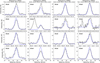 |
Fig. 1 Observed and modelled spectra of SO2 transitions towards o Ceti. The black line represents the observed spectrum, while the blue line represents the modelled spectrum. The strong line at 296.5500 GHz, shown in the second subplot of the third row from the bottom, represents the SO line. The narrow line in the last subplot of the same row corresponds to TiO2 (331.5996 GHz). |
3 Results
Figure 1 depicts the observed and modelled spectra towards o Ceti. The spectra of other sources are provided in the appendix (see Figs. B.1 and B.2). Table A.1 summarizes all the detected transitions. The line width (FWHM), ΔV, VLSR, and the integrated intensity (∫Tmbdv) of each transition were measured by applying a single Gaussian to fit the observed spectrum. The line parameters of all the observed transitions such as the rest frequency (ν0), quantum numbers ( ), FWHM, ∫Tmbdv, upper state energy (Eup), and VLSR are noted in Table A.1.
The rotational diagrams of SO2 and 34SO2 (when available) are shown in Figs. 2, 3, 4, 5, and 6 for o Ceti, R Leo, R Dor, W Hya, and EP Aqr, respectively. Table 3 compares the derived excitation temperatures and column densities from both RD and MCMC methods. The results of individual sources are discussed in the following subsections.
3.1 o Ceti
Many transitions of SO2 (16 lines), 34SO2 (14 lines), SO (3 lines), and 34SO (2 lines) are detected with a wide range of upper state energy (Eup ~ 40-700 K; see Table A.1). Additionally, we detected one transition of 33SO (343.0861 GHz). We also find a line close to the frequency of a 33SO2 line (345.5852 GHz), but do not associate it with 33SO2 emission because other lines potentially expected to be seen (at 283.338 GHz, 296.270 GHz, 334.030 GHz, and 479.960 GHz) are not observed. We have multiple transitions of SO2 and 34SO2 , and hence applied a rotation diagram analysis (see Fig. 2). The rotational diagram analysis yields excitation temperatures and column densities of Tex = 542 ± 168 K and NSO2 = (7.06 ± 3.55) × 1016 cm−2 for SO2 and Tex = 214 ± 71 K and N34SO2 = (2.16 ± 0.87) × 1015 cm−2 for 34SO2. Our estimated temperature of SO2 is comparable with the previous measurement based on TiO (474 ± 69) K (Kaminski et al. 2017) and AlF observations within uncertainties (Saberi et al. 2022). For o Ceti, a very faint signal at 493.3622 (Eup ≈ 564 K) GHz transition of H2S is observed towards the central source, but it is below the detection limit. Assuming LTE, we created synthetic spectra to match the observed profile. For this, we adopted the same temperature of 542 K, obtained from the RD of o Ceti, and estimated the upper limit for the column density of H2S to be 6.53 × 1014 cm−2. However, we did not detect any signal of the high-excitation transition (Eup ≈ 564 K) towards the arc-like structure of o Ceti. Danilovich et al. (2017b) found that H2S likely plays an important role in oxygen-rich AGB stars with high mass-loss rates, but is unlikely to be significant in stars of other chemical types or in oxygen-rich stars with lower mass-loss rates.
Figures C.1-C.3 show the moment 0 maps of all detected transitions (also see Fig. 1 in the supplementary document). A spatial analysis with high-resolution (~0.2″) observations in different ALMA bands shows centralized emission for all transitions with emitting regions around ~ 1″ towards the main continuum source. The shape of the emission shows irregular appearances, which could be due to the binary companion. The average separation between binary sources is 0.472″ (Vlemmings et al. 2015), corresponding to ~48 au, considering a distance of 102 pc. Nonetheless, we cannot distinguish the distinct features of SO and SO2 around Mira A and B with the present angular resolution.
Furthermore, for several transitions (Eup < 200 K) we find extended emission in the south-west position, which is completely offset and unconnected to the emission that is close to the continuum peak. For example, the low-excitation transitions of SO and SO2 (see Figs. C.4 and C.5) show an extended emission, about 3″ (~ 300 au) offset from the continuum position. Because of the lower intensity of the offset emission, it does not appear as a prominent feature in the integrated intensity maps. Hence, we plotted channel maps for these transitions, in which the extended emission is more clearly visible. In these figures, we see the extended feature in a few channels around ±3 km s−1 of the VLSR = 47 km s−1. Previously, Wong et al. (2016) reported the extended spatially resolved emission in SiO ( J = 5-4) ALMA observation around the same position. Our observations show SO and SO2 emissions around the same region where SiO appears. Since SiO is a good tracer of shocks (Fontani et al. 2019), the formation of gas-phase SO and SO2 is probably caused by shock-induced processes in the same environment. It could also be a region with higher gas density. The morphological correlation between SO, SO2, and SiO emissions implies that the shock processes might enhance the gas-phase abundance of these molecules. Shocks can significantly influence chemistry by increasing temperatures and densities and disrupting dust grains. In particular, shock waves can sputter dust grains and ice mantles (Suutarinen et al. 2014), releasing sulphur-bearing species such as atomic sulphur (S), hydrogen sulphide (H2S), or sulphur monoxide (SO) into the gas phase. These species can then undergo rapid gas-phase reactions to form SO2. Furthermore, we estimated that the temperature of this region is ~133 ± 20 K, based on an LTE analysis of all detected transitions of SO and SO2 towards the offset position (see Table A.2.)
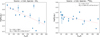 |
Fig. 2 Rotational diagram of SO2 and 34SO2 for o Ceti. The filled blue squares represent the data points, and the vertical lines on each data point indicate the error bars. The solid red lines represent the fitted line. |
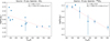 |
Fig. 3 Rotational diagram of SO2 and 34SO2 for R Leo. The filled blue squares represent the data points, and the vertical lines on each data point indicate the error bars. The solid red lines represent the fitted straight line. |
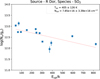 |
Fig. 4 Rotational diagram of SO2 for R Dor. The filled blue squares represent the data points, and the vertical lines on each data point indicate the error bars. The solid red line represents the fitted straight line. |
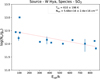 |
Fig. 5 Rotational diagram of SO2 for W Hya. The filled blue squares represent the data points, and the vertical lines on each data point indicate the error bars. The solid red line represents the fitted straight line. |
Rotational temperature and column density of SO2 and 34SO2 from two methods.
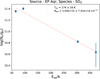 |
Fig. 6 Rotational diagram of SO2 for EP Aqr. The filled blue squares represent the data points, and the vertical lines on each data point indicate the error bars. The solid red line represents the fitted straight line. |
3.2 R Dor
A list of detected transitions of SO2 (14 lines), 34SO2 (2 lines), SO (1 line), and 34SO (1 line) towards R Dor is provided in Table A.1. We applied rotational diagram analysis for SO2 to obtain the excitation temperature (see Fig. 4). Our derived excitation temperature is Tex= 405±126 K and NSO2 = (7.85 ± 3.39) × 1016 cm−2. We do not have multiple transitions of 34SO2 and SO. Hence, we measured the excitation temperature and the column density of these species using the MCMC method. Our estimated excitation temperature using SO2 is consistent with previous measurements: ~505 K (Khouri et al. 2024). Moment 0 maps of different transitions of SO2 are shown in Fig. C.6 (also see Fig. 2 in the supplementary document). It is clear from Fig. 2 in the supplementary document that SO2 is unresolved with ACA observation, but with high-resolution data it is well resolved and shows clumpy emission structures (see Fig. C.6) where the continuum peak is at the centre. Furthermore, emission shows more compact features for transitions with high upper-state energy than the lower Eup transition. Our results, obtained at an angular resolution of 0.2″, are consistent with previous ALMA observations at a comparable resolution (~0.15″) (Danilovich et al. 2020). The co-spatial emission of SO and SO2 (see Fig. C.6) suggests that both molecules trace the same wind structure within the circumstellar environment. Furthermore, since the MRS of our observations is approximately 3″, we compared the observed intensities of transitions with similar Eup in our data and previous results obtained using the APEX 12m single-dish telescope (Danilovich et al. 2016). This comparison was performed to determine whether any flux has been resolved out in the interferometric data. However, we found good agreement between the single-dish and interferometric results for transitions with comparable Eup.
3.3 R Leo
All detected transitions of SO2 (10 lines), 34SO2 (7 lines), SO (1 line), and 34SO (1 line) towards R Leo are summarized in Table A.1. We have multiple transitions of SO2 and 34SO2. Hence, we applied a rotational diagram to estimate the excitation temperature and column density (see Figs. 3). The rotational diagram analysis yields excitation temperatures and column densities of Tex = 393 ± 112 K and NSO2 = (1.91 ± 0.83) × 1016 cm−2 for SO2 and Tex = 363 ± 53 K and N34SO2 = (1.85 ± 0.44) × 1015 cm−2 for 34SO2. For SO, we do not have multiple transitions. Consequently, we employed the MCMC method to derive a column density of SO of 6.3 × 1015 cm−2 and an excitation temperature of Tex = 300 K. Figures C.7 and C.8 (also see Fig. 3 in the supplementary document) show moment 0 maps of all detected transitions of SO2, 34SO2, SO, and 34SO. It is clear from Fig. 3 in the supplementary document that emission of SO2 is not resolved with a low-resolution (~2.6″) observation. In contrast, SO2 can be resolved well with high-resolution (~0.22″) data, as is shown in Figs. C.7 and C.8. We find a morphological correlation in the emission between SO2, 34SO2, and SO. The emission from the low-excitation transitions of (Eup = 81 K) and 34SO2 (Eup = 77 K) appears to be slightly more extended compared to higher-excitation transitions. Overall, the emission from both SO and SO2 is centrally concentrated and co-spatial, suggesting that these species likely trace the same wind structures in the CSE of R Leo.
3.4 W Hya
The observed transitions of SO2 (13 lines) and 34SO2 (3 lines) towards W Hya are noted in Table A.1. The estimated excitation temperature using the SO2 rotational diagram is Tex = 610 ± 198 K and the column density NSO2 = (5.68 ± 2.4) × 1016 cm−2. Moment 0 maps for different transitions of SO2 with high-(~0.16″) and low-resolution (~2.0″) observations are depicted in Fig. C.9 and Fig. 4 in the supplementary document, respectively. In the case of W Hya, emission from SO2 is not resolved in the ACA observations, similar to R Dor and R Leo. However, we find an additional structure of strong SO2 emission located approximately 10″ offset from the central continuum peak. It possibly traces the structures at the outer envelope of W Hya. At high resolution, the SO2 emission is resolved. It exhibits an ordered, centrally concentrated structure, with a slight offset between the continuum and molecular emission peak, similar to what is observed in R Leo. However, we do not detect the additional features at the offset position, which we found from ACA observations. The structure at the offset position is most likely resolved out due to the limited MRS of 2.1″ in the highresolution observations. We do not have an SO transition in the frequency range of our observation. Nonetheless, modelling results from previous studies suggest that the SO2 distribution is similar in size and abundance to the circumstellar SO distribution (Danilovich et al. 2016).
3.5 EP Aqr
For EP Aqr, we have several transitions of SO2 (five lines) and one transition of 34SO2 (one line) but only with ALMA Band 8 ACA observations (see Table A.1). The rotational diagram yields Tex= 174±16 K and NSO2 = (1.02 ± 0.74) × 1015 cm−2. Figure 5 in the supplementary document shows the moment 0 maps of SO2 transitions. The slightly lower temperature obtained compared to other sources (see Table 3) could be due to the large emission regions and the lack of high-resolution data with multiple transitions for this source. All transitions are spatially unresolved because of the low angular resolution of ~2.5″. Tuan-Anh et al. (2019) reported one transition of SO2 and found that the emission is confined towards the centre of the source, with an emitting diameter of ~0.25″ (~30 au). They suggest that SO2 could be a useful tracer of the mass-loss mechanism in its early phase. Their analysis also provided clear evidence of rotation, possibly combined with moderate expansion. Furthermore, by applying the temperature radial dependence from Hoai et al. (2019) and considering the radial extent of the SO2 emission, they estimated a gas temperature of a few hundred Kelvin, consistent with values typical of oxygen-rich AGB stars (Yamamura et al. 1999). However, a multi-transition (with a wide range of Eup) with high-angular resolution observations could provide better constraints on both the spatial distribution and the actual gas temperature traced by SO2.
4 Discussion
4.1 SO and SO2 distributions
SO and SO2 have previously been found by Danilovich et al. (2016) and Wallström et al. (2024) to have centralized distributions for low-mass-loss rate AGB stars and shell-like distributions for high-mass-loss sources. They also observed that sources with shell-like emission are typically detected in lower-energy SO2 lines, while those with centralized emission are more often detected in higher-energy lines. All five stars in our sample have relatively low mass-loss rates. We investigated the distribution of SO2 and SO towards these sources. For o Ceti, we observe slightly irregular emission contours for SO2, 34SO2, SO, and 34SO, and emission peaks are offset from the continuum peak. The emissions of SO2 and 34SO2 are spatially correlated, as are the emissions of SO and 34SO. However, with the current angular resolution, we cannot distinguish the distributions of our detected species between the Mira A and B components. Furthermore, we detected extended emission for several transitions of SO and SO2 and some other species (see Table A.2) at the south-west position, which is ~3″ offset from the main continuum and molecular emission peaks (e.g. see Figs. C.4 and C.5). The extended emission region is also seen with the SiO (5-4) transition (Wong et al. 2016), suggesting that shocks may play a significant role in the origin of SO and SO2. In addition, the measured temperature of this arc-like structure is lower than that of the central region. Distributions of 34SO and SO2 show a morphological correlation in R Dor. The emissions of these species are clumpy, but the emission peak appears at the centre of the continuum peak. For R Leo, we find ordered emission structures of SO2 and 34SO2 centred at the continuum peak. We find similar features for SO and 34SO but they are slightly extended compared to the SO2 and 34SO2 emission. SO and 34SO probably trace the cold gas of the outer layer of the CSE. In W Hya, we find SO2 and 34SO2 contours with an approximate circular pattern without smooth arcs, and emission peaks are slightly offset from the continuum peak. Apart from the central emission around the continuum peak, additional strong emission peaks appear to the north-west, which is 10″ offset from the continuum peak. SO2 and 34SO2 are not resolved with the ACA observations of EP Aqr. In summary, our results support the previous conclusion that SO and SO2 exhibit a centralized distribution in low-mass-loss rate AGB stars.
Recently, Danilovich et al. (2025) observed low-excitation (Elow < 100 K) transitions of SO2 towards the intermediate-mass AGB star OH 30.1-0.7. The source is thought to have a very high mass loss rate (>10−4 M⊙ yr−1). They found shell-like distributions of SO2, consistent with the morphology discussed above for sources with high-mass loss rates. Their results suggest a low excitation temperature for SO2 around the source. They also conclude that their result aligns with the observed trend that AGB stars with high-mass loss rates tend to show lower-energy SO2 transitions (Wallström et al. 2024). In contrast, we have detected both low- and high-excitation transitions in a sample of AGB stars with low mass-loss rates. We obtained high excitation temperatures of SO2 for all sources (see Table 3), of the order of a few hundred Kelvin, indicating that SO2 originates mainly from the intermediate region of the CSE in all sources. The average high angular resolution of our observations is ~0.2″ and the MRS -3″. Since the emitting regions of the detected species are confined to within ~ 2.0″ (see Figs. C.1, C.2, C.3, C.6, C.7, C.8, and C.9), and the MRS is consistently higher than this, we can assume that we have recovered all of the flux. Therefore, we do not expect significant flux loss due to spatial filtering.
The centralized emission of SO and SO2 towards o Ceti, W Hya, and R Leo could be due to several physical properties of their surrounding environments. Khouri et al. (2018) found dust surrounding both Mira A and B, as well as a dust tail connecting the two stars. They found a region around Mira A that exhibits high gas density close to the star, which is characterized by a steep decline in density at its outer edge. Mira is a binary system, and within this context, the observed SO and SO2 emission is centrally concentrated but displays an irregular morphology, suggesting that their formation in the inner envelope might be influenced by both local density enhancements and dynamical effects related to binarity. R Leo has an episodic and patchy mass ejection circumstellar environment (Hoai et al. 2023), leading to localized shocks in the inner envelope, which in turn may enhance SO and SO2 formation, producing the observed centralized emission. The CSE of the stable component of W Hya shows an approximately spherical morphology, with the gas and dust expanding radially (Hoai et al. 2022). The SO and SO2 emissions are centrally concentrated, indicating an origin in the warm, dense inner envelope, where possibly shocks and dust-formation processes predominate in sulphur chemistry.
Ionization effects are likely to play only a minor role in these sources, as the species reside in the inner envelope, where they are expected to be shielded from the interstellar radiation field. Furthermore, the centralized SO and SO2 emissions indicate that these molecules are not primarily produced by outer-shell photochemistry. However, the present data cannot resolve the molecular emission features between the individual components in sources with binary companions. Furthermore, the modelling results of Danilovich et al. (2016) found that, in their sample of low-mass-loss-rate stars, both SO and SO2 exhibit centrally peaked abundance distributions. In contrast, in higher-mass-loss rate stars, the SO abundance peaks further out in the wind. The SO2 abundance profile might follow a similar profile (Danilovich et al. 2020). However, dedicated studies of individual sources, combining observations and modelling, are needed to better understand the origin of emission features of sulphur-bearing molecules.
4.2 Sulphur isotopic ratio in various astrophysical environments
All sources in our sample are oxygen-rich AGB stars with a similar metallicity and mass-loss rates of approximately 10−7 M⊙ yr−1 (see Table 1). We estimated the 32S/34S ratio for o Ceti and R Leo using column density values that were obtained using RD analysis, and for W Hya, R Dor, and EP Aqr values obtained using MCMC analysis. Our measured isotopic ratios with their uncertainties are listed in Table 3. We estimated a 32S/34S ratio of 32±6 for o Ceti, 10±3 R Leo, 26±8 for R Dor, 18±4 for W Hya, and 12±5 for EP Aqr. Comparing these ratios with the solar value of 21.7, our estimated values for R Dor and W Hya are in good agreement with the solar value. The ratios for EP Aqr and R Leo are slightly lower, and for o Ceti, it is slightly higher than the expected value. We also measured 33S/34S ratio ~0.35 for o Ceti, which is higher than the solar value (- 0.17, Asplund et al. 2021) by a factor of 2. However, this is only in one source and based on one line of 33SO. Hence, we need multitransition observations to constrain this ratio and to compare this with different astrophysical environments.
Along with SO2 and 34SO2 transitions, we also have one pair of SO and 34SO detection towards o Ceti, R Leo, and R Dor. In the case of o Ceti, an approximate 32SO/34SO ratio of 7±1 was obtained using the integrated intensities of transitions with similar Eup and transition probabilities. This is considerably lower than the ratio of 32.4 obtained from SO2 isotopologue ratio. This could be partly due to opacity effects, which we did not take into account in our calculations. The emitting regions of two molecules may also differ, leading to the over- or underestimation of the column densities and derived isotopic ratios. For R Dor, we have one transition of SO with high Eup = 143 K and 34SO with low Eup = 80 K. Also, their transitions are very different. Hence, we did not estimate the 32SO/34SO. Our measured value of 32SO/34SO is 6.0±0.5 for R Leo, which was obtained using integrated intensities of two transitions with a similar Eup and transition probability This value is also considerably lower than the value of 26 obtained from the SO2 isotopologue ratio, likely for the same reason as was discussed for o Ceti.
Our measured value of 32 SO2 /34 SO2 towards two oxygenrich AGB stars, R Dor and W Hya, agrees well with the solar value within the uncertainties, indicating that 32S and 34S are not significantly processed during the AGB phase. However, the measured ratio for o Ceti is slightly higher and for R Leo and EP Aqr the measured ratios are lower. The obtained value of the 32S/34S ratio in R Leo and IRC-10529 is significantly lower than the solar value, which can be attributed to the fact that these sources might have a lower metallicity or have formed in an environment with lower 32 S/34 S. Another possibility could be the age effect of the different environments. Conversely, our estimated 32SO/34SO ratio deviates from the solar value, which could be attributed to the SO line being optically thick. In such cases, the observed line intensity underestimates the true SO column density, leading to an artificially low isotopic ratio. To verify the accuracy of the 32S/34S ratio obtained here, it would be useful to derive the sulphur isotopic ratio using other sulphur-bearing species abundant in the CSEs of oxygenrich AGB stars, such as CS and SiS, in addition to SO and SO2, as was previously performed by Velilla Prieto et al. (2017) for IK Tau.
Furthermore, we compared our derived 32S/34S ratios with different astrophysical environments (see Fig. 7), such as the Large Magellanic Cloud (LMC), representing a low-metallicity environment with a metallicity of ~0.3-0.5 Z⊙ (Westerlund 1997); starburst galaxies, NGC 253 with a metallicity of ~0.5-1.5 Z⊙ (Beck et al. 2022); NGC 4945 with a metallicity of ~0.5-1.2 Z⊙ (Mouhcine et al. 2005; Stanghellini et al. 2015); the Milky Way (the central part has solar metallicity and decreasing metal-licity with distance), considering different environments; the outer Galaxy has a metallicity similar to the LMC (Shimonishi et al. 2021), the local interstellar medium (ISM); the inner disc; the CMZ; the Solar System; and finally, a list of AGB stars that includes our work and some literature values. It is clear from Figure 7 that the 32S/34S ratios for most of the Galactic AGB stars except R Leo and IRC-10529 are comparable to the solar value, including different environments from our Galaxy and Solar System. Since 32S and 34S are primarily produced through explosive nucleosynthesis during Type II and Type Ia SNe, the measured values in AGB stars reflect the abundances in their natal clouds. In contrast, 32S/34S ratios in LMC and starburst galaxies are lower compared to the solar value. Based on comprehensive calculations, Woosley & Weaver (1995) reported that 32S and 33S are the primary yield (in the sense that the stellar yields do not strongly depend on the initial metallicity of the stellar model) and do not depend on the initial metallicity of the stellar yield, i.e. metal content of a star at its birth, while 34S is not a clean primary isotope, and its yield decreases with metallicity. Recently, Gong et al. (2023) also reported that 32S/33S and 34S/33S in the LMC are lower than in the Milky Way and NGC 253 and concluded that this can be attributed to a combination of age (the LMC may be composed of older stellar populations that have not undergone as much recent nucleosynthesis), low metallicity (which influences the types and outcomes of nuclear reactions in stars), and the star formation history (e.g. rate of star formation).
The 32S/34S isotopic ratio shows an increasing trend from NGC 253 (youngest evolutionary stage) to the Milky Way (oldest) (see Fig. 7), which may correlate with the age of stellar populations across these galaxies. NGC 253, a starburst galaxy with the lowest 32S/34S ratio, is dominated by massive young stars due to intense recent star formation, which may indicate minimal isotopic processing. NGC 4945, with a slightly higher 32S/34S ratio, has a mix of younger and older stars, reflecting a moderately older stellar population than NGC 253. The LMC, with an even higher 32S/34S ratio, contains stars that are several billion years old, making it older than NGC 4945 but younger than the Milky Way. The Milky Way, with the highest 32S/34S ratio, hosts the oldest stellar populations, including stars that are over 13 billion years old, suggesting significant nucleosyn-thetic evolution. This trend indicates that lower 32S/34S ratios are associated with younger, less processed stellar populations. In contrast, higher ratios correspond to older, more evolved galactic environments where sulphur chemistry has been processed significantly. However, this analysis is based on a small sample. Therefore, we need a large sample and systematic analysis to confirm this trend with different multi-transition sulphur-bearing species along with different isotopic ratios such as 33S/34S, 32S/33S, and 32S/34S.
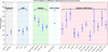 |
Fig. 7 32S/34S ratios for different environments. N113 - Gong et al. (2023); ST11, ST16 - Shimonishi et al. (2020); NGC 253 - Martín et al. (2021); NGC 4945 - Wang et al. (2004); Solar System - Anders & Grevesse (1989); CMZ, inner disc, local ISM, outer Galaxy - Yan et al. (2023); IRC+10216 - Mauersberger et al. (2004); W Aql, IRC+10011, IRC-10529 - Wallström et al. (2024); 15194-5115, 15082-4808, 07454-7112 - (Unnikrishnan et al. 2024); o Ceti, R Dor, W Hya, R Leo, EP Aqr - This work. Additionally, Danilovich et al. (2020) reported a ratio of 42 for the Galactic AGB star, IK Tau, which is not included in the plot due to the absence of measured uncertainties. |
5 Conclusions
We have analysed the data of five oxygen-rich AGB stars with low resolution (~2.5″) and complementary high resolution (~0.2″), obtained with the ALMA ACA and 12m array. The major conclusions of this paper are summarized as follows:
We report the detection of 16 transitions of SO2, 14 of 34SO2, 3 of SO, and 2 of 34SO towards o Ceti; 14 transitions of SO2, 2 of 34SO2, and 1 transition each of SO and 34SO towards R Dor; 10 transitions of SO2, 7 of 34SO2, and 1 transition each of SO and 34SO towards R Leo; 13 transitions of SO2 and 3 of 34SO2 towards W Hya; and 5 transitions of SO2 and 1 of 34SO2 towards EP Aqr;
We estimate the excitation temperature using detected sulphur-bearing species to be around 200-600 K across different sources and report column densities of - (1-7)× 1016 cm−2 for SO2 and ~ (0.8-3) × 1015 cm−2 for 34SO2. Based on the spatial distribution analysis and temperature measurement, we conclude that the detected molecule traces the intermediate region (-50-500 au away from the central star) of the CSE;
We measure the 32S/34S ratios for five sources, and two of them, R Dor and W Hya, are found to be close to the solar value within uncertainties. For o Ceti, it is slightly higher, and for R Leo and Ep Aqr, the ratios are slightly lower. Overall, 13 Galactic AGB stars have measured 32 S/34 S ratios (see Fig. 7), of which 8 are consistent with the solar value within the uncertainties, while 5 show some variations. It is believed that nucleosynthesis in AGB stars does not significantly alter the sulphur isotopic ratio, and the observed values are expected to reflect the abundances of their natal clouds. Therefore, the observed discrepancies in the 32S/34S ratios among Galactic AGB stars may arise from assumptions of solar metallicity, which might not hold universally, and/or variations in the excitation conditions within their CSEs. Further analysis using different sulphur-bearing species is needed to provide deeper insights, which is beyond the scope of this work;
We find that SO2, 34SO2, SO, and 34SO emission contours are slightly irregular and the emission peaks are offset from the continuum peak of o Ceti. We report an extended emission structure towards the south-west, offset by ~3″ (-300 au) from the continuum peak, where emissions of SO and SO2 correlate with SiO molecular distribution (Wong et al. 2016). This region exhibits several transitions of SO and SO2 and some other species reported in Table A.2, likely enhanced by shock chemistry and most probably a low-velocity shock. We estimate the temperature of the arc-like emission to be -133 ± 20 K;
SO and 34SO2 show clumpy structures in R Dor, with the peak of the molecular emission centred on the continuum peak. Our results are consistent with a previous study by Danilovich et al. (2020);
The emission of SO2, 34SO2, SO, and 34SO transitions in R Leo appear as ordered elliptical concentric emission contours and molecular emission peak slightly offset from the continuum peak. Similar to o Ceti, low-excitation transitions in R Leo show a slightly extended feature in moment 0 maps compared to higher-energy transitions;
The distribution of SO2 and 34 SO2 in W Hya appears as ordered approximately circular concentric emission contours, and where the emission peak is slightly offset from the continuum peak as o Ceti. Furthermore, we find an additional structure of strong SO2 emission located in the north-west, which is ~ 10″ (~1040 au) offset from the central continuum peak;
For EP Aqr, we have only low-resolution data with which SO2 and 34SO2 are mostly unresolved. Hence, we cannot provide a detailed insight into the distribution of detected species;
In summary, we have studied five oxygen-rich AGB stars with comparable low mass-loss rates and find some differences in the distribution and morphology of the emissions from SO2, 34SO2, SO, and 34SO across different sources. These differences are likely due to the chemistry being highly sensitive to the physical conditions of the sources, such as the density and temperature structures of the CSEs, source multiplicity, outflows, rotation, and other physical processes associated with the sources. Nonetheless, the mostly centralized distributions of SO and SO2 in our sample support previous results for low-mass-loss rate AGB stars.
Data availability
The data underlying this article (as presented in the appendix) are available on Zenodo under a Creative Commons Attribution license at https://zenodo.org/records/17302962
Acknowledgements
This paper makes use of the following ALMA data: ADS/JAO.ALMA#2018.1.01440.S, #2018.1.00649.S, #2018.1.00749.S, #2018.1.00649.S,#2016.1.01202.S, #2017.A.00012.S, #2019.1.00801.S. ALMA is a partnership of ESO (representing its member states), NSF (USA) and NINS (Japan), together with NRC (Canada), MOST and ASIAA (Taiwan), and KASI (Republic of Korea), in cooperation with the Republic of Chile. The Joint ALMA Observatory is operated by ESO, AUI/NRAO, and NAOJ. P.G. and M.S. acknowledge the ESGC project (project No. 335497) funded by the Research Council of Norway. TD is partly supported by the Australian Research Council through a Discovery Early Career Researcher Award (DE230100183).
References
- Anders, E., & Grevesse, N. 1989, Geochim. Cosmochim. Acta, 53, 197 [Google Scholar]
- Asplund, M., Amarsi, A. M., & Grevesse, N. 2021, A&A, 653, A141 [NASA ADS] [CrossRef] [EDP Sciences] [Google Scholar]
- Beck, A., Lebouteiller, V., Madden, S. C., et al. 2022, A&A, 665, A85 [NASA ADS] [CrossRef] [EDP Sciences] [Google Scholar]
- Danilovich, T., De Beck, E., Black, J. H., Olofsson, H., & Justtanont, K. 2016, A&A, 588, A119 [NASA ADS] [CrossRef] [EDP Sciences] [Google Scholar]
- Danilovich, T., Lombaert, R., Decin, L., et al. 2017a, A&A, 602, A14 [NASA ADS] [CrossRef] [EDP Sciences] [Google Scholar]
- Danilovich, T., Van de Sande, M., De Beck, E., et al. 2017b, A&A, 606, A124 [NASA ADS] [CrossRef] [EDP Sciences] [Google Scholar]
- Danilovich, T., Ramstedt, S., Gobrecht, D., et al. 2018, A&A, 617, A132 [NASA ADS] [CrossRef] [EDP Sciences] [Google Scholar]
- Danilovich, T., Richards, A. M., Decin, L., van de Sande, M., & Gottlieb, C. A. 2020, MNRAS, 494, 1323 [NASA ADS] [CrossRef] [Google Scholar]
- Danilovich, T., Richards, A. M. S., Van de Sande, M., et al. 2025, MNRAS, 536, 684 [Google Scholar]
- De Nutte, R., Decin, L., Olofsson, H., et al. 2017, A&A, 600, A71 [NASA ADS] [CrossRef] [EDP Sciences] [Google Scholar]
- Fontani, F., Rivilla, V. M., van der Tak, F. F. S., et al. 2019, MNRAS, 489, 4530 [CrossRef] [Google Scholar]
- Fontani, F., Roueff, E., Colzi, L., & Caselli, P. 2023, A&A, 680, A58 [NASA ADS] [CrossRef] [EDP Sciences] [Google Scholar]
- Francis, L., Johnstone, D., Herczeg, G., Hunter, T. R., & Harsono, D. 2020, AJ, 160, 270 [NASA ADS] [CrossRef] [Google Scholar]
- Ghosh, R., Das, A., Gorai, P., et al. 2024, Front Astron Space Sci, 11, 1427048 [Google Scholar]
- Goldsmith, P. F., & Langer, W. D. 1999, ApJ, 517, 209 [Google Scholar]
- Gong, Y., Henkel, C., Menten, K. M., et al. 2023, A&A, 679, L6 [NASA ADS] [CrossRef] [EDP Sciences] [Google Scholar]
- Hinkle, K. H., Lebzelter, T., & Straniero, O. 2016, ApJ, 825, 38 [NASA ADS] [CrossRef] [Google Scholar]
- Hoai, D. T., Nhung, P. T., Tuan-Anh, P., et al. 2019, MNRAS, 484, 1865 [NASA ADS] [CrossRef] [Google Scholar]
- Hoai, D. T., Tuyet Nhung, P., Darriulat, P., et al. 2022, Vietnam J. Sci., 64, 16 [Google Scholar]
- Hoai, D. T., Nhung, P. T., Tan, M. N., et al. 2023, MNRAS, 518, 2034 [Google Scholar]
- Kaminski, T., Müller, H. S. P., Schmidt, M. R., et al. 2017, A&A, 599, A59 [NASA ADS] [CrossRef] [EDP Sciences] [Google Scholar]
- Khouri, T., Vlemmings, W. H. T., Olofsson, H., et al. 2018, A&A, 620, A75 [NASA ADS] [CrossRef] [EDP Sciences] [Google Scholar]
- Khouri, T., Olofsson, H., Vlemmings, W. H. T., et al. 2024, A&A, 685, A11 [NASA ADS] [CrossRef] [EDP Sciences] [Google Scholar]
- Krijt, S., Kama, M., McClure, M., et al. 2023, in Astronomical Society of the Pacific Conference Series, 534, Protostars and Planets VII, eds. S. Inutsuka, Y. Aikawa, T. Muto, K. Tomida, & M. Tamura, 1031 [Google Scholar]
- Lindqvist, M., Nyman, L. A., Olofsson, H., & Winnberg, A. 1988, A&A, 205, L15 [Google Scholar]
- Martín, S., Mangum, J. G., Harada, N., et al. 2021, A&A, 656, A46 [NASA ADS] [CrossRef] [EDP Sciences] [Google Scholar]
- Massalkhi, S., Agúndez, M., Cernicharo, J., & Velilla-Prieto, L. 2020, A&A, 641, A57 [NASA ADS] [CrossRef] [EDP Sciences] [Google Scholar]
- Mauersberger, R., Ott, U., Henkel, C., Cernicharo, J., & Gallino, R. 2004, A&A, 426, 219 [NASA ADS] [CrossRef] [EDP Sciences] [Google Scholar]
- McMullin, J. P., Waters, B., Schiebel, D., Young, W., & Golap, K. 2007, in Astronomical Society of the Pacific Conference Series, 376, Astronomical Data Analysis Software and Systems XVI, eds. R. A. Shaw, F. Hill, & D. J. Bell, 127 [Google Scholar]
- Mifsud, D. V., Kaåuchová, Z., Herczku, P., et al. 2021, Space Sci. Rev., 217, 14 [CrossRef] [Google Scholar]
- Mouhcine, M., Rich, R. M., Ferguson, H. C., Brown, T. M., & Smith, T. E. 2005, ApJ, 633, 828 [Google Scholar]
- Müller, H. S. P., Thorwirth, S., Roth, D. A., & Winnewisser, G. 2001, A&A, 370, L49 [Google Scholar]
- Müller, H. S. P., Schlöder, F., Stutzki, J., & Winnewisser, G. 2005, J. Mol. Struct., 742, 215 [Google Scholar]
- Nhung, P. T., Hoai, D. T., Winters, J. M., et al. 2015, A&A, 583, A64 [NASA ADS] [CrossRef] [EDP Sciences] [Google Scholar]
- Omont, A., Lucas, R., Morris, M., & Guilloteau, S. 1993, A&A, 267, 490 [NASA ADS] [Google Scholar]
- Saberi, M., Khouri, T., Velilla-Prieto, L., et al. 2022, A&A, 663, A54 [NASA ADS] [CrossRef] [EDP Sciences] [Google Scholar]
- Shimonishi, T., Das, A., Sakai, N., et al. 2020, ApJ, 891, 164 [NASA ADS] [CrossRef] [Google Scholar]
- Shimonishi, T., Izumi, N., Furuya, K., & Yasui, C. 2021, ApJ, 922, 206 [NASA ADS] [CrossRef] [Google Scholar]
- Stanghellini, L., Magrini, L., & Casasola, V. 2015, ApJ, 812, 39 [NASA ADS] [CrossRef] [Google Scholar]
- Suutarinen, A. N., Kristensen, L. E., Mottram, J. C., Fraser, H. J., & van Dishoeck, E. F. 2014, MNRAS, 440, 1844 [Google Scholar]
- Tuan-Anh, P., Hoai, D. T., Nhung, P. T., et al. 2019, MNRAS, 487, 622 [CrossRef] [Google Scholar]
- Unnikrishnan, R., De Beck, E., Nyman, L. Â., et al. 2024, A&A, 684, A4 [NASA ADS] [CrossRef] [EDP Sciences] [Google Scholar]
- Vastel, C., Bottinelli, S., Caux, E., Glorian, J. M., & Boiziot, M. 2015, in SF2A-2015: Proceedings of the Annual meeting of the French Society of Astronomy and Astrophysics, 313 [Google Scholar]
- Velilla Prieto, L., Sánchez Contreras, C., Cernicharo, J., et al. 2017, A&A, 597, A25 [NASA ADS] [CrossRef] [EDP Sciences] [Google Scholar]
- Vlemmings, W. H. T., Ramstedt, S., O’Gorman, E., et al. 2015, A&A, 577, L4 [NASA ADS] [CrossRef] [EDP Sciences] [Google Scholar]
- Vlemmings, W. H. T., Khouri, T., & Olofsson, H. 2019, A&A, 626, A81 [NASA ADS] [CrossRef] [EDP Sciences] [Google Scholar]
- Wallström, S. H. J., Danilovich, T., Müller, H. S. P., et al. 2024, A&A, 681, A50 [NASA ADS] [CrossRef] [EDP Sciences] [Google Scholar]
- Wang, M., Henkel, C., Chin, Y. N., et al. 2004, A&A, 422, 883 [NASA ADS] [CrossRef] [EDP Sciences] [Google Scholar]
- Westerlund, B. E. 1997, Cambridge Astrophys. Ser., 29 [Google Scholar]
- Wong, K. T., Kaminski, T., Menten, K. M., & Wyrowski, F. 2016, A&A, 590, A127 [NASA ADS] [CrossRef] [EDP Sciences] [Google Scholar]
- Woosley, S. E., & Weaver, T. A. 1995, ApJS, 101, 181 [Google Scholar]
- Yamamura, I., de Jong, T., Onaka, T., Cami, J., & Waters, L. B. F. M. 1999, A&A, 341, L9 [Google Scholar]
- Yan, Y. T., Henkel, C., Kobayashi, C., et al. 2023, A&A, 670, A98 [NASA ADS] [CrossRef] [EDP Sciences] [Google Scholar]
Appendix A Summary of detected species and their transitions
In this section we present the line parameters of all detected species towards a sample of five AGB stars and summary of detected transitions towards o Ceti arc-like structure
Line parameters of observed transitions towards our sample AGB stars.
Species detected towards o Ceti arc-like structure
Appendix B Observed and synthetic spectra
Here we present the synthetic spectra obtained with MCMC fitting and the observed spectra for R Dor, R Leo, W Hya, and Ep Aqr.
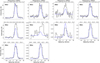 |
Fig. B.1 Observed and synthetic spectra of SO2 transitions towards R Dor. The black line represents the observed spectrum, while the blue line represents the modelled spectrum. |
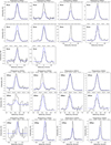 |
Fig. B.2 Observed and synthetic spectra of SO2 transitions towards R Leo, W Hya, and EP Aqr. The black line represents the observed spectrum, while the blue line represents the modelled spectrum. |
Appendix C Moment 0 and channel maps
In the appendix, we present moment 0 maps of all detected strong transitions, as well as channel maps of SO and SO2, which are provided to illustrate the extended atmosphere of o Ceti. Figures C.1, C.2, and C.3 show the moment 0 maps of the detected transitions towards o Ceti (one additional figure (Fig. 1) of moment 0 maps of SO2 is provided in the supplementary document). The channel maps of SO and SO2 are presented in Figures C.4 and C.5, respectively. Moment 0 maps of the detected transitions towards R Dor are shown in Figure C.6 (one additional figure (Fig. 2) of moment 0 maps of SO2 is provided in the supplementary document). For R Leo, the moment 0 maps are shown in Figure C.7 and C.8 (one additional figure (Fig. 3) of moment 0 maps of SO2 is provided in the supplementary document). Figure 4 in supplementary document and Fig. C.9 display the moment 0 maps of the transitions identified towards W Hya. Moment 0 maps of the detected transitions towards EP Aqr are available in the supplementary document (Fig. 5).
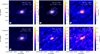 |
Fig. C.1 Moment 0 maps of SO2 transitions using ALMA Band 7 observations towards source o Ceti. Contours are drawn with steps of 3σ, 9σ, 18σ, 36σ, 48σ, 72σ, and 96σ. The beam size is shown at the lower left corner of each subplot as a filled grey ellipse. The cyan cross symbol indicates the position of the continuum peak. |
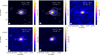 |
Fig. C.2 Moment 0 maps of SO and 34SO transitions using ALMA Band 7 observations towards source o Ceti. Contours are drawn with steps of 3σ, 9σ, 18σ, 36σ, 48σ, and 72σ. The beam size is shown at the lower left corner of each subplot as a filled grey ellipse. The cyan cross symbol indicates the position of the continuum peak. |
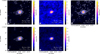 |
Fig. C.3 Moment 0 maps of SO2 transitions using ALMA Band 8 observations towards source o Ceti. Contours are drawn with steps of 3σ, 9σ, 18σ, 36σ, 48σ, 72σ, and 96σ. The beam size is shown at the lower left corner of each subplot as a filled grey ellipse. The cyan cross symbol indicates the position of the continuum peak. |
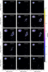 |
Fig. C.4 Channel maps of SO (JKa, Kc = 67 - 56) low excitation transition (Eup = 65 K) towards o Ceti. Contours are drawn with steps of 3σ, 4σ, 5σ, 6σ, 9σ, 12σ, 18σ, and 36σ. The beam size is shown at the lower left corner of each subplot as a filled grey ellipse. The cyan cross symbol indicates the position of the continuum peak. |
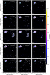 |
Fig. C.5 Channel maps of SO2 (JKa, Kc = 74,4 - 63,3) low excitation transition (Eup = 65 K) towards o Ceti. Contours are drawn with steps of 3σ, 4σ, 5σ, 6σ, 9σ, 12σ, 18σ, and 36σ. The beam size is shown at the lower left corner of each subplot as a filled grey ellipse. The cyan cross symbol indicates the position of the continuum peak. |
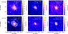 |
Fig. C.6 Moment 0 maps of SO2 transitions towards R Dor using ALMA 12m array observations. Contours are drawn with steps of 3σ, 4σ, 5σ, 6σ, 9σ, 12σ, 15σ, 18σ, and 24σ. The beam size is shown at the lower left corner of each subplot as a filled grey ellipse. The cyan cross symbol indicates the position of the continuum peak. |
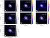 |
Fig. C.7 Moment 0 maps of SO2 transitions towards R Leo using ALMA 12m array observations. Contours are drawn with steps of 3σ, 4σ, 5σ, 6σ, 9σ, 12σ, 18σ, 36σ, 48σ, 72σ, and 96σ. The beam size is shown at the lower left corner of each subplot as a filled grey ellipse. The cyan cross symbol indicates the position of the continuum peak. |
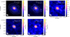 |
Fig. C.8 Moment 0 maps of SO, 34SO, and 34SO2 transitions towards R Leo using ALMA 12m array observations. Contours are drawn with steps of 3σ, 6σ, 9σ, 12σ, 18σ, 36σ, 48σ, 72σ, and 96σ. The beam size is shown at the lower left corner of each subplot as a filled grey ellipse. The cyan cross symbol indicates the position of the continuum peak. |
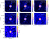 |
Fig. C.9 Moment 0 maps of SO2 transitions towards W Hya using ALMA 12m array observations. Contours are drawn with steps of 3σ, 4σ, 5σ, 6σ, 9σ, 12σ, 18σ, and 36σ. The beam size is shown at the lower left corner of each subplot as a filled grey ellipse. The cyan cross symbol indicates the position of the continuum peak. |
All Tables
All Figures
|
Fig. 1 Observed and modelled spectra of SO2 transitions towards o Ceti. The black line represents the observed spectrum, while the blue line represents the modelled spectrum. The strong line at 296.5500 GHz, shown in the second subplot of the third row from the bottom, represents the SO line. The narrow line in the last subplot of the same row corresponds to TiO2 (331.5996 GHz). |
| In the text | |
|
Fig. 2 Rotational diagram of SO2 and 34SO2 for o Ceti. The filled blue squares represent the data points, and the vertical lines on each data point indicate the error bars. The solid red lines represent the fitted line. |
| In the text | |
|
Fig. 3 Rotational diagram of SO2 and 34SO2 for R Leo. The filled blue squares represent the data points, and the vertical lines on each data point indicate the error bars. The solid red lines represent the fitted straight line. |
| In the text | |
|
Fig. 4 Rotational diagram of SO2 for R Dor. The filled blue squares represent the data points, and the vertical lines on each data point indicate the error bars. The solid red line represents the fitted straight line. |
| In the text | |
|
Fig. 5 Rotational diagram of SO2 for W Hya. The filled blue squares represent the data points, and the vertical lines on each data point indicate the error bars. The solid red line represents the fitted straight line. |
| In the text | |
|
Fig. 6 Rotational diagram of SO2 for EP Aqr. The filled blue squares represent the data points, and the vertical lines on each data point indicate the error bars. The solid red line represents the fitted straight line. |
| In the text | |
|
Fig. 7 32S/34S ratios for different environments. N113 - Gong et al. (2023); ST11, ST16 - Shimonishi et al. (2020); NGC 253 - Martín et al. (2021); NGC 4945 - Wang et al. (2004); Solar System - Anders & Grevesse (1989); CMZ, inner disc, local ISM, outer Galaxy - Yan et al. (2023); IRC+10216 - Mauersberger et al. (2004); W Aql, IRC+10011, IRC-10529 - Wallström et al. (2024); 15194-5115, 15082-4808, 07454-7112 - (Unnikrishnan et al. 2024); o Ceti, R Dor, W Hya, R Leo, EP Aqr - This work. Additionally, Danilovich et al. (2020) reported a ratio of 42 for the Galactic AGB star, IK Tau, which is not included in the plot due to the absence of measured uncertainties. |
| In the text | |
|
Fig. B.1 Observed and synthetic spectra of SO2 transitions towards R Dor. The black line represents the observed spectrum, while the blue line represents the modelled spectrum. |
| In the text | |
|
Fig. B.2 Observed and synthetic spectra of SO2 transitions towards R Leo, W Hya, and EP Aqr. The black line represents the observed spectrum, while the blue line represents the modelled spectrum. |
| In the text | |
|
Fig. C.1 Moment 0 maps of SO2 transitions using ALMA Band 7 observations towards source o Ceti. Contours are drawn with steps of 3σ, 9σ, 18σ, 36σ, 48σ, 72σ, and 96σ. The beam size is shown at the lower left corner of each subplot as a filled grey ellipse. The cyan cross symbol indicates the position of the continuum peak. |
| In the text | |
|
Fig. C.2 Moment 0 maps of SO and 34SO transitions using ALMA Band 7 observations towards source o Ceti. Contours are drawn with steps of 3σ, 9σ, 18σ, 36σ, 48σ, and 72σ. The beam size is shown at the lower left corner of each subplot as a filled grey ellipse. The cyan cross symbol indicates the position of the continuum peak. |
| In the text | |
|
Fig. C.3 Moment 0 maps of SO2 transitions using ALMA Band 8 observations towards source o Ceti. Contours are drawn with steps of 3σ, 9σ, 18σ, 36σ, 48σ, 72σ, and 96σ. The beam size is shown at the lower left corner of each subplot as a filled grey ellipse. The cyan cross symbol indicates the position of the continuum peak. |
| In the text | |
|
Fig. C.4 Channel maps of SO (JKa, Kc = 67 - 56) low excitation transition (Eup = 65 K) towards o Ceti. Contours are drawn with steps of 3σ, 4σ, 5σ, 6σ, 9σ, 12σ, 18σ, and 36σ. The beam size is shown at the lower left corner of each subplot as a filled grey ellipse. The cyan cross symbol indicates the position of the continuum peak. |
| In the text | |
|
Fig. C.5 Channel maps of SO2 (JKa, Kc = 74,4 - 63,3) low excitation transition (Eup = 65 K) towards o Ceti. Contours are drawn with steps of 3σ, 4σ, 5σ, 6σ, 9σ, 12σ, 18σ, and 36σ. The beam size is shown at the lower left corner of each subplot as a filled grey ellipse. The cyan cross symbol indicates the position of the continuum peak. |
| In the text | |
|
Fig. C.6 Moment 0 maps of SO2 transitions towards R Dor using ALMA 12m array observations. Contours are drawn with steps of 3σ, 4σ, 5σ, 6σ, 9σ, 12σ, 15σ, 18σ, and 24σ. The beam size is shown at the lower left corner of each subplot as a filled grey ellipse. The cyan cross symbol indicates the position of the continuum peak. |
| In the text | |
|
Fig. C.7 Moment 0 maps of SO2 transitions towards R Leo using ALMA 12m array observations. Contours are drawn with steps of 3σ, 4σ, 5σ, 6σ, 9σ, 12σ, 18σ, 36σ, 48σ, 72σ, and 96σ. The beam size is shown at the lower left corner of each subplot as a filled grey ellipse. The cyan cross symbol indicates the position of the continuum peak. |
| In the text | |
|
Fig. C.8 Moment 0 maps of SO, 34SO, and 34SO2 transitions towards R Leo using ALMA 12m array observations. Contours are drawn with steps of 3σ, 6σ, 9σ, 12σ, 18σ, 36σ, 48σ, 72σ, and 96σ. The beam size is shown at the lower left corner of each subplot as a filled grey ellipse. The cyan cross symbol indicates the position of the continuum peak. |
| In the text | |
|
Fig. C.9 Moment 0 maps of SO2 transitions towards W Hya using ALMA 12m array observations. Contours are drawn with steps of 3σ, 4σ, 5σ, 6σ, 9σ, 12σ, 18σ, and 36σ. The beam size is shown at the lower left corner of each subplot as a filled grey ellipse. The cyan cross symbol indicates the position of the continuum peak. |
| In the text | |
Current usage metrics show cumulative count of Article Views (full-text article views including HTML views, PDF and ePub downloads, according to the available data) and Abstracts Views on Vision4Press platform.
Data correspond to usage on the plateform after 2015. The current usage metrics is available 48-96 hours after online publication and is updated daily on week days.
Initial download of the metrics may take a while.