| Issue |
A&A
Volume 704, December 2025
|
|
|---|---|---|
| Article Number | A191 | |
| Number of page(s) | 19 | |
| Section | Planets, planetary systems, and small bodies | |
| DOI | https://doi.org/10.1051/0004-6361/202556033 | |
| Published online | 16 December 2025 | |
Search for exocomet transits in Kepler light curves
Ten new transits identified
1
Institut d’astrophysique de Paris, CNRS, Sorbonne Université,
98 bis boulevard Arago,
75014
Paris,
France
2
CRAL, Ecole normale supérieure de Lyon, Université de Lyon, UMR, CNRS 5574,
69364
Lyon Cedex 07,
France
3
LIRA, Observatoire de Paris, Université PSL, CNRS, Sorbonne Université, Université de Paris,
5 place Jules Janssen,
92195
Meudon,
France
4
Institut Pierre-Simon Laplace, Sorbonne-Université, CNRS,
Paris,
France
★ Corresponding author: This email address is being protected from spambots. You need JavaScript enabled to view it.
Received:
19
June
2025
Accepted:
15
October
2025
Abstract
Although the Kepler telescope was retired over a decade ago, it continues to offer a rich dataset for uncovering new astrophysical objects and phenomena. In this study, we conducted a comprehensive search for exocometary transit signatures within the Kepler light curves, using a machine learning approach based on a neural network trained on a library of theoretical exocomet transit light curves. By analyzing the light curves of 201 820 stars, we identified candidate events through the neural network and subjected the output to filtering and visual inspection to mitigate false positives. Our results are presented in three catalogs of increasing ambiguity. The first tier catalog includes 17 high-confidence exocometary transit events, comprising seven previously reported events and ten newly identified ones, each associated with a different host star. The second tier catalog lists 30 lower-confidence events that remain consistent with possible exocometary transits. The third tier catalog consists of 49 more symmetric photometric events that could be exocometary transits, exoplanet mono-transits, or false positives due to eclipsing binaries mimicking transits. Contrary to previous studies, which suggested that the cometary activity was favored by stellar youth, we find a broad age distribution among candidate host stars, including several red giants. This challenges the general idea of a decline in cometary activity with stellar age and underlines the need for further investigation into the temporal evolution of exocometary activity in planetary systems.
Key words: methods: data analysis / techniques: photometric / surveys / comets: general
© The Authors 2025
 Open Access article, published by EDP Sciences, under the terms of the Creative Commons Attribution License (https://creativecommons.org/licenses/by/4.0), which permits unrestricted use, distribution, and reproduction in any medium, provided the original work is properly cited.
This article is published in open access under the Subscribe to Open model. This email address is being protected from spambots. You need JavaScript enabled to view it. to support open access publication.
1 Introduction
Exocomets are rocky or icy minor bodies that become active when they approach their parent star on a highly eccentric orbit (Strøm et al. 2020). Because they produce a huge tail of gas and dust close to periastron, when they transit in front of the star, they become detectable using spectroscopy (for the gaseous tail) and photometry (for the dust tail). The first exocomets were thus identified in the 1980s in the β Pic system, through the detection of variable absorption features in the Ca II lines of the stellar spectrum (Ferlet et al. 1987; Kiefer et al. 2014a). Later on, a few other exocometary systems were found using spectroscopy, for example HD 172555 (Kiefer et al. 2014b; Grady et al. 2018) and 49 Cet (Montgomery & Welsh 2012; Miles et al. 2016). A list of spectroscopically identified exocometary systems can be found in Strøm et al. (2020).
For the detection of exocomets using photometry, one needs to obtain photometric measurements at high accuracy, typically at the 10−3−10−4 level over the full transit duration, i.e., for one to three days (Lecavelier des Etangs et al. 1999, hereafter LdE99a). This capability was reached only during the last decade with space missions such as Corot, Kepler, TESS, and Cheops. Detections have thus been obtained with Kepler toward KIC 3542116 and KIC11084727 (Rappaport et al. 2018), and KIC8027456 (Kennedy et al. 2019), with TESS toward β Pic (Zieba et al. 2019; Pavlenko et al. 2022; Lecavelier des Etangs et al. 2022), and with Cheops toward HD 172555 (Kiefer et al. 2023). Here we also mention the detection with Kepler of a photometric event, possibly periodic, which has been interpreted as the transit of a string of five to seven exocomets in front of KIC 8462852 (Kiefer et al. 2017).
All these events were identified thanks to the particular shape of the light curve of an exocomet transit, as theoretically predicted at the end of the 1990s in LdE99a: the characteristic of an exocomet transit light curve is the asymmetry caused by the cometary tail passing in front of the star after the nucleus. This causes a sharp decrease in the star light followed by a slow return to the normal brightness (see also Lecavelier des Etangs 1999, hereafter LdE99b). However, exocomet transit light curves can also be more symmetric when the longitude of the periastron of the orbit is about 90° from the line of sight, because here the cometary tail is aligned with the line of sight. In this case, the shape of the transit light curve is similar to that of an exoplanet transit (LdE99a).
The detection of exocometary transits based on photometry is complementary to the detection through spectroscopy. It allows the physical characteristics of dust particles to be explored, such as the dust particle size distribution, the distance to the host star at the time of transit, and the dust production rate (Luk’yanyk et al. 2024). Because transits give direct access to the geometrical extent and the optical thickness of the transiting dust cloud, coupled with models of dust production, this allows the estimate of the dust production rate and the size of the comets nucleus. In the case of β Pic, a statistical analysis of the photometric events allowed the estimate of the nucleus size distribution that was found to be similar to that of asteroids and comets in the Solar System as set by collisional equilibrium (Lecavelier des Etangs et al. 2022).
Although the characterization of exocomets paves the way to understanding the dynamical and chemical processes occurring in young planetary systems, only a very limited number of exocometary systems have been identified to date. As a result, our current understanding of the diversity, frequency, and evolutionary significance of exocometary activity remains incomplete. Systematic searches have been performed using spectroscopy in the Ca II line (Montgomery & Welsh 2012; Welsh & Montgomery 2013, 2018; Rebollido et al. 2020; Bendahan-West et al. 2025), resulting in a few detections (see review in Strøm et al. 2020). Spectroscopy is efficient in detecting tiny amounts of gas, and thus allows a sensitive search; the result is that detectable spectroscopic transits seem to be more frequent than detectable photometric events. For instance, in the case of β Pic, several exocomet transits are routinely detected every day in spectroscopy (Kiefer et al. 2014a), while only 30 photometric transits were detected in 156 days of TESS observations (Lecavelier des Etangs et al. 2022). However, spectroscopic searches for exocomets are inherently limited by their need to observe each target star individually and the need for long observation times with high spectral resolution. In contrast, photometric surveys can monitor several thousand stars simultaneously, making them significantly more efficient for large-scale searches for exocometary transits.
In that spirit, Rappaport et al. (2018) and Kennedy et al. (2019) began a deep search for exocometary transits in the Kepler light curves. To identify exocometary transits, they used a modified model of planetary transit or a combination of exponential and Gaussian tails, as also done later on by Zieba et al. (2019), Pavlenko et al. (2022), and Lecavelier des Etangs et al. (2022). Although this empirical approach does not carry physical information about the cometary bodies and tails, it is easy to implement and thus to identify candidates in the large number (~200 000) of light curves provided by Kepler.
Here we propose to use an automated search without the use of analytical functions to describe the exocometary transit light curves. For that we combined a search algorithm based on a neural network together with a library of photometric transits to train the network. The library is an updated version of the library of LdE99b, which has been recalculated using faster CPUs than those used 20 years ago, covering a wide range of parameters, and therefore a wide range of transit shapes that need to be identified. We applied this automated search to the Kepler data (Borucki et al. 2010) with the aim of producing a new catalog of exocometary system candidates. The methods are described in Sects. 2-4. The search in the Kepler data is presented in Sect. 5. The final catalog of candidates, divided into three tiers, is given in Sect. 6. The results are discussed in Sect. 7.
2 Training of the neural network
2.1 Training principle
The method used for the detection of exocomets in the Kepler data is based on a neural network using supervised learning. For the network learning, we used a library of theoretical light curves divided into three disjoint sets of labeled light curves: the training set, the validation set, and the test set. Each set contains the same number of light curves with and without an exocomet transit (see Sect. 2.2). Each light curve is labeled to indicate if it includes a transit or not.
Our objective is to make the algorithm identify the curves containing an exocomet transit among all the light curves collected by the Kepler satellite and to recover the transit time when a transit is present. Using an iterative procedure, the algorithm optimizes its parameters thanks to the training set. At the end of each iteration step called an epoch, the network performance is tested using the validation set. This allows us to control the overfitting of the algorithm (e.g., it becomes specific to the training set and loses in generality) and to adjust the hyperparameters. The learning phase is stopped when the network shows the best performance in the validation set. The final performance of the algorithm is given by its evaluation on the test set.
2.2 Light curve production
The light curves used to build the training, validation, and test set are the Presearch Data Conditioning (PDC) data from Kepler Data Release 25 (Thompson et al. 2016). We used the Quarters 1 to 17 and divided them into subquarters in case of interruption of the acquisition within a given quarter: two subquarters are separated by at least four consecutive photometric measurements missing in the light curve.
For each subquarter, a training, validation, and test set were constructed to overcome their possible specificity. For each subquarter, the training set consists of 36 000 curves, while the validation and test sets contain 12 000 each. A curve consists of ten days (480 photometric measurements at a cadence of one measurement every ~30 minutes) of acquisition of the luminosity flux from a star randomly chosen without repetition.
To ensure efficient learning and prevent the algorithm from falling into obvious traps, several modifications were applied to the Kepler PDC data. First, all data points deviating by more than 5σ from the mean of the light curve were removed, provided that their neighboring points remained within the 5σ range. In addition, each curve was normalized to have a zero mean and a standard deviation of 1, as needed for optimal learning by the algorithm. Finally, the possible missing measurements, i.e., at most three consecutive missing measurements within the same subquarter, were filled using a linear interpolation.
For the learning process, half of the ten-day light curves were labeled “0”, indicating the absence of an exocomet transit. Given that the probability of a randomly selected Kepler light curve containing an exocomet transit is extremely low, we assume that all light curves labeled “0” are free of exocometary transits. This subset was used to train the algorithm to learn the intrinsic noise patterns in the Kepler data. For the remaining half of the ten-day light curves, we added one synthetic exocomet transit by multiplying the light curve by a transit from the theoretical library (Sect. 2.3), and labeled these curves “1”, indicating the presence of an exocomet transit.
2.3 Simulation of exocomet transits
In order for the algorithm to learn to identify the shape of an exocomet transit in the light curves, we added theoretical exocomet transits to half of the curves that make up the training data. These theoretical exocomet transit light curves were calculated using the method described in LdE99a. We produced a library of 2200 exocomet transit light curves, which is an updated version of the library published 20 years ago by LdE99b. Among all the available simulations, we selected only those with a gas production rate log10(P/(1kg s−1)) between 6 and 7.5 and an impact parameter b < R*, where R* is the radius of the star. This choice guarantees that the used transit light curves are sufficiently deep.
An impact parameter greater than one stellar radius or a production rate that is too low leads to a noisy and very weak extinction and would therefore have no interest for the training. Before adding the simulated transits to the Kepler light curves, we multiplied the theoretical transit light curve by a random constant such that the depth of the transits is in the interval [2σ, K + 2σ] where K is the depth of the simulated transits and σ the standard deviation of the Kepler light curves. We thus trained our model for a signal-to-noise ratio higher than 2 to exclude the cases where the transit would not be detectable. The transit times of the theoretical transits added to the ten-day light curves are chosen randomly, with a uniform distribution between the beginning and the duration of the simulated transit before the end of the light curve.
Finally, in order to ensure that the training data are representative of the diversity of possible transits, we used a uniform random distribution of the distance of the periastron q in the set {0.2; 0.3,; 0.5; 0.7; 1.0} astronomical units and of the longitude of the periastron ω from −157.5° to +157.5° with a step of 22.5°, as in LdE99b.
The theoretical transits that have been used are totally different from the training, validation and the test sets. To guarantee that the evaluation of the algorithm’s performance is unbiased, the choice of the transits for each set was made randomly from the whole set of theoretical transits.
3 The neural network model
3.1 Architecture
The deep learning algorithm developed in this study is mainly based on the convolution layer sequence adapted for pattern recognition. We relied on the architecture of existing algorithms for the detection of exoplanet transits (Shallue & Vanderburg 2018; Dattilo et al. 2019; Zucker & Giryes 2018; Chintarungruangchai & Jiang 2019). These algorithms, which all have a similar architecture, are optimized for periodic transit detection. They have been modified to be efficient for the detection of single transits as the orbital period of an exocomet is expected to be much longer than the Kepler mission duration. Two major modifications have been made. Squeeze-excited blocks (Hu et al. 2018) have been added to the convolution blocks. The authors indeed show that such blocks can improve the performance of a pattern-matching algorithm by improving the interdependence relations between the convolution layers without adding computational cost. The addition of the long short-term memory (LSTM) (Hochreiter & Schmidhuber 1997) and the gated recurrent unit (GRU) (Cho et al. 2014) layers also resulted in significant performance improvements. The algorithm was implemented in TensorFlow, an open-source machine learning framework (Abadi et al. 2016). We optimized the neural network parameters thanks to KerasTuner (O’Malley et al. 2019).
Figure 1 describes our final model, which is mainly a onedimensional convolutional network. The activation function of all the convolutional layers is the rectified linear unit (ReLU) function (Jarrett et al. 2009). The output is a list of two real numbers. The first uses a sigmoid function whose range is (0,1). It is the probability returned by the algorithm that the ten-day input light curve contains an exocomet transit. An output value close to 1 indicates high confidence that the considered light curve has one transit, while an output value close to 0 means that there is no transit. The second output layer is activated by a linear function in the range (0,1). It gives the position of the identified transit in the light curve. If no transit is detected, the layer should return a value close to zero.
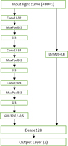 |
Fig. 1 Architecture of our best performing neural network model. The input data is a light curve of 480 timesteps, the output is a list of two real numbers between 0 and 1: one for the probability of detection of an exocometary transit and one for the position of the transit in the light curve. Convolutional layers are denoted Conv <kernel size> <number of feature maps>, max pooling layers are denoted MaxPool <window length> <stride length>, fully connected layers are denoted Dense <number of units>, LSTM layers are denoted LSTM <units> <dropout>, GRU layers are denoted GRU <unit> <droupout> <recurent dropout>, and the squeezed-excitation blocks are denoted SEB. |
3.2 Training
For each subquarter, we trained the model using 36 000 light curves for 150 training epochs, which means that we performed 150 complete passes through the entire training dataset to update the model weight parameters. We used the Adam optimization algorithm (Kingma & Ba 2015) to minimize the cross-entropy error function for the classification of the light curves and the mean absolute error function for the position of the transit. We used a learning rate of 10−4 and a batch size of 5000. The saved model in the one for which the validation loss reaches its minimum; it is usually obtained after 50-80 iterations (epochs). Therefore, training the model over 150 epochs is considered sufficient.
4 Evaluation of the neural network performance
We evaluated the performance of our neural network with respect to several metrics in the same way as Dattilo et al. (2019) did for their model. We computed all the metrics over the test set (rather than the training or validation sets) to avoid using any data that were used to optimize the parameters or hyperparameters of the model.
4.1 The metrics
The metrics used to evaluate the performance of a classifier are the following:
Accuracy, the fraction of curves correctly classified by the model;
Precision (reliability), the fraction of correctly classified exocomets, i.e., the fraction of curves classified as exocomet candidates (False positives + True positives NFp + NTp) that are indeed true positives (1-labeled):
 (1)
(1)Recall (completeness or true-positive rate), the fraction of the curves 1-labeled, which therefore includes an exocomet transit (true positives + false negatives, NTp + NFn), that the model classifies as exocomet candidates (NTp):
 (2)
(2)False-positive rate (FPR), the fraction of total 0-labeled curves, which therefore do not include any exocomet transit (false positives +true negatives, NFp + NTn) that the model classifies as exocomet candidates:
 (3)
(3)Area under the receiver-operator characteristic curve (AUC; see Figure 2), the probability that the model, if it receives two light curves, one 1-labeled curve including an exocomet transit and one 0-labeled curve without transit, would rank the 1-labeled curve higher than the 0-labeled curve;
Mean absolute error, the absolute error for all 1-labeled curves between the true position of the transit and the predicted position by the model.
The first five metrics are related to the detection of the presence of an exocomet in the light curves, while the last metric is related to the position in time of the transit in the light curve. Except for the AUC, the values of these metrics depend on the classification threshold chosen for the model. This threshold is the value of the probability of detection yield by the algorithm above which we consider that there is a detection. In Fig. 2 we show the evolution of the recall as a function of the FPR for various thresholds, usually called the receiver-operator characteristic (ROC) curve. It can be seen that the algorithm differentiates well between true transits and noise, as it achieves very low FPR recall, while keeping a reasonably large recall; our model reaches an AUC of 98.88% for the quarter Q1. We also plot the precision as a function of the recall. This curve shows the trade-off between having no false positives (high precision) and identifying all exocomet transits (high recall).
Considering the huge number of light curves in the Kepler data, the goal was to drastically reduce the number of false positives. We thus chose a classification threshold of 0.99. With this threshold, our model reaches an accuracy of 89.5% for the quarter Q1. The precision of the model is 99.8%, which means that we reach a high true positive rate, and the recall is 79.1%, which means that about 20% of the true exocomet transits are missing in the final classification. This trade-off aims to accept some loss in the finding of exocomet transits of about 20% to avoid a large number of false positives. Given the large number of light curves in the Kepler data and the small number of exocomet transits in these data, even a tiny fraction of false positives can significantly pollute the results. The metrics values are found to be similar for all quarters (see Table A.1).
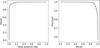 |
Fig. 2 Receiver-operator characteristic curve (left panel) and the precision vs. recall curve (right panel). The ROC curve shows the recall (true-positive rate) of the model against the ability to recognize false positives (false-positive rate) for different classification thresholds. Our model is highly successful at identifying false positives, as shown by the high AUC value (see Table A.1). The plot of the fraction of exocomets that the model classified as exocomets (recall) vs. the fraction of correctly classified planets (precision) shows the trade-off between having no false positives (high precision) and identifying all exocomet transits (high recall). |
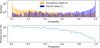 |
Fig. 3 Histogram of the results on the test set and error on the transit position found by the network. Top panel: histogram of the result of the neural network applied to the test data. Most of the 1-labeled light curves with an exocomet transit yield a probability close to 1, while there are only a few false positives (0-labeled light curves yielding a high probability). Above the chosen threshold, there is more than two order of magnitude between the number of true positives and false positive. Bottom panel: mean error of the position of the transit as a function of the probability of the presence of a transit assigned by the network to the light curves. This error is a few hours at most for the transits identified by the algorithm. |
4.2 Quality of the output
The quality of the model classification can also be visualized by the histogram of the results on the test set (top panel of Fig. 3). The closer the output from the neural network is to 1 (resp. 0), the higher the probability that the ten-day light curve contains (resp. does not contain) an exocomet transit. The histogram shows that the neural network works as expected: on the left-hand side, most of the light curves characterized by a low probability are mostly noise (orange histogram), while on the right-hand side, the large majority of the curves characterized by a probability close to 1 include a simulated exocomet transit (label 1; blue histogram) and with very few false positives. The bottom graph of Fig. 3 shows the mean error of the position of the transit as a function of the probability assigned by the algorithm when it is applied to the curves containing a simulated transit (label 1, with known position). One can see that when the transit is not found (probability close to 0), the error on the predicted position is large, about 3 days, whereas it is on the order of a few hours only when the probability is above 0.99. Thus, one can be confident in the time of the transit given by the algorithm for curves with a probability higher than this threshold.
5 Search for exocomets in Kepler data
5.1 Application of the model to Kepler data
To apply the algorithm presented in the previous sections, all the light curves of the Kepler data were cut into ten-day windows obtained in the same way as the samples used to construct the training, validation, and test sets described in Sect. 2.2. In order not to lose any transits located at the edge of the windows, an overlap of 2 days was applied between two consecutive ten-day time intervals.
However, despite the level of precision achieved, the algorithm provided a large number of false positives due to the large number of ten-day windows: approximately 106 windows per quarter lead to about 103 positive candidate detections, among which less than a dozen real transits should be identified (see LdE99a and discussion in Sect. 7). To reduce the number of false positives, we decided to filter the candidates using constraints on the shape of the light curves of the detected photometric events.
5.2 Additional criteria to filter false positives
After all the Kepler light curves have passed through the neural network, we end up with a set of 56 525 exocomet candidates. To filter these candidates, we decided to add constraints on the shape and on the context on the transit (noise, quality flags).
5.2.1 Filtering through the shape of the transit candidates
The shapes of the candidate transits were determined by fitting them via the model proposed by Lecavelier des Etangs et al. (2022) together with a second-order polynomial baseline:
 (4)
(4)
The parameters t0 and t1 represent respectively the time at which the transit starts and the time at which it reaches its minimum; K represents the characteristic depth of the transit, while 1/β corresponds to the characteristic crossing time of the transit; and C, D, and E are the coefficients of the polynomial baseline. The fit of the light curve by the transit model can be easily performed using the position of the detected candidate in the light curve as provided by the network output.
To accept or reject a proposed detection given by the neural network, we fit the light curve of the corresponding photometric event to obtain the values of the parameters K, β, and ΔT = t1 − t0 that characterize the shape of the event.We then check that these values are in the domain of validity for an exocometary transit. The domain of validity is obtained by considering the parameters space occupied by the fits of the theoretical light curves in the library of numerical simulations of exocometary transits, as shown in Fig. 4 and summarized in the first three lines of Table 1.
It is found that in the theoretical light curves K is mostly between 10−4 and 5 × 10⁻³, ∆T is between 1.7 and 17 hours (corresponding to a periastron between ~0.02 to 2 au, Lecavelier des Etangs et al. 2022), and β−1 is in the domain above 0.5 hours, and between 0.3∆T − 1.7 and 0.5∆T + 12. Moreover, the parameters C and D have to verify the condition |C|, |D| < 10−3. This ensures that the background is stable enough in the neighborhoods of the transit. When this is not the case, the detected transit appears to be only noise.
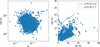 |
Fig. 4 Distribution of the value of the parameters obtained by fitting the 2163 light curves in the library of the simulated exocomet transits. The parameters K, ∆T = t1 − t0, and 1/β correspond to the depth, ingress duration, and crossing time of the transit, respectively. |
5.2.2 Quality flags
We observed that the presence of certain quality flags indicates an alteration of the light curve leading to a systematic detection by the network. Thus, candidates whose transit position is less than 1 day away from a quality flag 3 (spacecraft is in coarse point) or 12 (impulsive outlier removed before cotrending) were discarded from the candidate list.
5.2.3 Presence in the list of KOIs
To avoid periodic transits, which constitute roughly half of the candidate transits output by the algorithm, stars belonging to the list of Kepler objects of interest (KOIs) were also removed.
5.2.4 Other cases of false positives
We found three other circumstances that can mislead the algorithm and then result in obvious false positives: (1) significant background noise on a timescale close to that of a cometary transit; (2) a ramp-like shape in the light curve, i.e., a very sudden decrease in flux followed by a more or less rapid return to the normal level; (3) the presence of a mono-transit of a possible exoplanet that results in a very symmetrical brightness dip. In the following, we suggest the criteria to address each of these three cases.
To characterize the presence of noise anomaly, the ∆rms was calculated. It is defined as
 (5)
(5)
where fexo(ti) is the exocomet model fit to the flux where the candidate transit is found, F3 is the mean of the flux without the three lowest points, and σ is the standard deviation of the flux. Only candidate transits with Δrms > 36 were conserved. This criterion was very useful to remove candidates that were detected due to a few points significantly lower than the average.
To detect the presence of red noise that mimics an exocomet transit, we calculated the correlation product between the exocomet model fit to the candidate transit and the light curve over all the considered subquarters. If the maximum of the correlation max1 is reached more than one day away from the transit time or if its second maximum max2 is significantly close to the first maximum ((max1 − max2)/max1 < 0.15), the candidate is removed, considering that in this case the noise in the light curve resembles the identified transit, which is therefore probably not a real exocomet transit, but background red noise.
The cases of the ramp-like light curves mimicking an exo-cometary transit have been discarded by calculating the difference between the fit with a comet model (Eq. (4)) and a fit with a simple ramp model defined as
 (6)
(6)
We calculate  defined as
 (7)
(7)
where N = 120 is the number of points in the fitted window.
The photometric events that are almost as well fit with the ramp model as with the exocomet model ( ) were discarded from the candidate list.
Finally, to identify the cases of a symmetrical transit that could be due to the passage of an exoplanet with a long period (a mono-transit), we calculated the difference  between the
  of a model of a planetary transit calculated using the equations of Mandel & Agol (2002) and the
  of an exocomet transit model (Eq. (4)). It can be written as
 (8)
(8)
The photometric events having  have a symmetrical shape and were therefore not taken into account in our final selection of exocomets. Such transits were taken into account to establish the list of symmetrical mono-transits (see Sect. 6.3).
However, this criterion is not used as a sharp cut to distinguish the exocomet transits from the symmetrical mono-transits but only as a help. The final distinction is made through visual inspection.
After applying these criteria, the number of candidate transits per quarter varies between 50 and 100 per quarter, leading to a total of 1349 transits. It then becomes possible to proceed for each of them to a visual inspection to know if the candidate is or is not an exocomet transit. This final inspection is necessary because, although the criteria put in place make it possible to eliminate the vast majority of false positives, there still remain obvious false positives. We note here that the criteria were deliberately chosen to be conservative so as not to accidentally eliminate a true exocomet transit. The number of criteria was chosen so that the final number of transits to be visually inspected would be no more than a few thousand. Otherwise, visual inspection would be impractical. It would be more inefficient and inaccurate to add extra criteria than to visually check the current list of 1349 transits.
To verify the robustness of the detected transits, we performed an additional test. We applied our detection procedure to the data after reversing the time. If the proportion of detected exocomets is the same in the reversed time data as in the original data, this may question the relevance of the detected transits. However, as this analysis is time-consuming, we performed this analysis on one-half of the quarters. Of the 17 quarters, we analyzed eight randomly chosen quarters: Q1, Q2, Q6, Q9, Q10, Q12, Q15, and Q16. We found only one transit that clearly mimics an exocomet transit: KIC_3129239 in Q9. Given that approximately 17 robust transits were detected in the Kepler data (see Sect. 6), we can infer from this study that about 10-15% of these transits can be false positives. Although the same number of detections in the time-reversed data would have disproven the exocomet hypothesis, the result of this test supports the idea that there is an astrophysical signal in the data that is consistent with exocomet transits.
Parameter values for filtering the candidate transits.
6 A new catalog of transiting exocomets
In this section we present the final list of exocomet transits resulting from the selection procedure. We divided the list into three different tiers based on the likelihood of a genuine exocometary detection. In the first tier, the photometric events are the ones that we consider as the most likely due to the transit of an exocomet. The second tier is for the events possibly due to comets, while the third tier gathers the most symmetric dip in the light curve, for which the transit of an exoplanet remains a possibility.
First tier catalog of exocometary transits.
6.1 The first tier catalog of exocometary transits
The first tier catalog of detected exocometary transits is given in Table 2 and the plots of the corresponding light curves are given in Appendix B. It is particularly noteworthy that our neural network is able to find all the transits already identified by previous works: KIC3542116 in Quarters 1, 10, and 12; KIC 11084727 as found by Rappaport et al. (2018); and KIC 8027456 as found by Kennedy et al. (2019). This independent retrieval of the same exocometary transits provides confidence in our procedure.
Nonetheless, after application of all the search procedure described above, it appeared that two transits of KIC 3542116 identified by Rappaport et al. (2018) in Quarters 8 were not in our list of detections. These transits were eliminated by the criterion based on the maximum of the correlation product that aims to remove the detections whose pattern occurs several times in the same subquarter (Sect. 5.2.4). This criterion also has the disadvantage of eliminating active cometary systems where at least two comet transits occurred in the same quarter, as is the case for KIC 3542166 in Quarter 8. Therefore, we made a visual inspection of all photometric events eliminated because of this criterion in order to recover possible obvious exocometary transits that were wrongly rejected. We thus found the two transits of KIC 3542116 in Quarter 8, and in addition identified a new transit in front of KIC 6263848. This last case does not correspond to a star with frequent cometary transits, but one that had been deleted due to an edge effect on the calculation of the correlation function. These two cases are flagged by an asterisk in Table 2.
For all of these detection, we calculate the  defined as
 (9)
(9)
where fpolynomial is the second-order polynomial that best fits the detection. For all detections, we obtained large  (larger than about 100). This highlights that the detection cannot be interpreted just as noise patterns.
The properties of the parent stars of the identified exocomets as tabulated by Kepler are given in Table 3 (Brown et al. 2011). For KIC 3542116 and KIC 3662483, the values for Teff, log10 g, metallicity, and radius are from Zhang et al. (2025). From the Teff and log10 g we can obtain an estimate of the stellar type (Gray 2008), which is given in the last column of Table 3. It appears that most of the stars are main-sequence stars, with the exception of KIC 4078638, which is likely a red giant. For these stars, the upper limits on the age estimate given by Zhang et al. (2025) are all above 109 years, with the exception of KIC 4481029 with an upper limit of 9 × 10⁸ years and KIC 8027456 with an age estimate of 5 × 10⁸ years.
6.2 The second tier catalog of possible exocometary
After visual inspection of the list of candidates produced by our algorithm, we came up with a list of interesting photometric events that can be due to transiting exocomets. This includes transits that pass through all the criteria described in Sect. 5, but whose shape or signal-to-noise ratio makes it difficult to decide whether they are actually transits. The resulting list of possible exocometary transits in this second tier catalog is given in Table 4, and the plots of the corresponding light curves are given in Appendix C.
The properties of the corresponding parent stars in the second tier catalog are given in Appendix D (Brown et al. 2011). Here again, estimates of the stellar types given in the last column of the table show that most of the stars are on or close to the main sequence, with the exception of KIC 2984102 and KIC 11153134, which have a log10 g below 3 and are therefore likely red giants. For all stars in this second tier catalog, the upper limit of the age estimate given by Zhang et al. (2025) is above 109 years, with the exception of KIC 2984102, KIC 5294231, and KIC 7183123 with age estimates of 5 × 10⁸, 1 × 10⁸ (with an upper limit of 3 × 10⁸), and 9 × 10⁸ years, respectively.
Information on the stars in the first tier catalog.
6.3 The third tier catalog of symmetric transits
After visual inspection of the list of candidates produced by our algorithm, we also came up with a list of interesting photometric events that appears to be symmetrical. This is not surprising as some of the exocomet transits in the library used for training the network are indeed symmetrical (see Figs. 2 and 3 in LdE99a). However, we cannot exclude that these are due to mono-transits of exoplanets or to false positives mimicking planetary or cometary transits. Several scenarios might cause such false positives, including diluted or undiluted eclipsing binaries. To identify these cases it would be necessary to carry out additional analyses that are beyond the scope of the present paper (see, e.g., Crossfield et al. 2016). Finally, although an exocometary transit classification cannot be made, these detections deserve to be mentioned. They are given in the third tier catalog of symmetric transits listed in Appendix E.
We compared these detected photometric events with the lists of single transits published by Huang et al. (2013), Wang et al. (2015), Foreman-Mackey et al. (2016), and Herman et al. (2019). It appears that four events in our list were already identified by Foreman-Mackey et al. (2016) and Herman et al. (2019). The transit in front of KIC 8410697 was found in both studies. It is interpreted as being due to an exoplanet with a radius that is 0.7 times that of Jupiter. The photometric event of KIC 10321319 was found by Foreman-Mackey et al. (2016) and is interpreted as being due to the transit of an exoplanet of 0.16 Jupiter radius. The photometric event of KIC 6196417 was found by Herman et al. (2019) and interpreted as being due to the transit of an exoplanet of about 0.7 Jupiter radius. The transit in front of KIC 10668646 at the time of BKJD=1449.3 was already identified by Foreman-Mackey et al. (2016), but the exoplanet transit scenario was rejected because of a centroid shift in the data. However, we also identified another photometric event in the same target at BKJD=196.3 with a different shape and a lower absorption depth. These few examples show that our list of newly identified photometric events that could be due to transits of exocomet with symmetrical shape of the light curve deserves further investigations, which are beyond the scope of the present paper.
7 Conclusion
Although the Kepler mission ended more than 10 years ago, the available data is still worth deep data mining in search of new discoveries. Here we presented a new search for exocometary transits in the Kepler light curves. We used a machine learning technique with a neural network trained using a library of theoretical exocomet transit light curves inherited from the work of LdE99b. After parsing the light curves of close to 200 000 stars through the neural network, despite the application of several filters to eliminate most of the false positive, a visual inspection of the outcome of the network was still needed. We ended up with three catalogs of interesting objects. The first tier catalog is composed of a total of 17 exocometary transits, including seven previously identified transits and ten new transits in front of ten different stars. The second tier catalog is a list of 30 photometric events that appear to be of second quality and that we qualify as possible exocometary transits. Finally, the third tier catalog presents the list of interesting photometric events that are symmetrical and may be due to transits of either an exoplanet or an exocomet with a periastron at 90° from the line of sight.
The complete Kepler data represent a four-year photometry survey of more than 170000 distinct stars. However, as noted in Kennedy et al. (2019), not all stars were observed for the full duration of the mission. As a result, we can consider 150 000 as the approximate number of equivalent stars that were observed for the full duration of the mission. In other words, our analysis covers the equivalent of about 600 000 star-years. LdE99a showed that, for a survey covering 30000 star-years of targets with Solar System-like cometary activity and achieving a photometric precision of a few 10−4, the expected number of exocomet transit detections is on the order of ten. Therefore, assuming that each star harbors a cometary system similar to our own, we could expect roughly 200 detections with a perfect search in the Kepler data. Finding a few dozen exocometary transits can therefore be considered a satisfactory result in agreement with what could be expected using reasonable estimates of the algorithm efficiency and cometary activity of the surveyed stars.
LdE99a showed that, for a survey covering 30 000 star-years of targets with Solar System-like cometary activity and achieving a photometric precision of a few 10−4, the expected number of exocomet transit detections is on the order of ten.
Unfortunately, the Kepler stars are rather faint, and our catalogs contain stars with magnitude between 9.7 and 15.9. It is therefore not possible to undertake a spectroscopic follow up with the hope of confirming the exocometary nature of the photometric events. All the more because with only one transit per star in about four years, exocometary transits are rare and not predictable in time. However, we can anticipate that the same techniques could be applied to search for exocometary transits in the current TESS data and in upcoming PLATO data. For these two instruments, the surveyed star in the input catalog are significantly brighter that the Kepler stars. We can thus expect that the exocometary systems to be discovered in the near future can be studied in detail, particularly through spectroscopy.
Previous searches (Rappaport et al. 2018; Kennedy et al. 2019) provided a list of three stars that seem to be rather young. This supported the anticipated conclusion that cometary activity is likely correlated with stellar age, with an expected decline over time. However, our catalogs do not support this idea; we found a wide spread of age for both the first and second tier catalogs, with possible exocometary transits in front of stars classified as red giants. The issue of cometary activity with age thus remains open, and further studies will be needed to clarify this important question of the evolution of planetary systems.
Note added to proofs. After this manuscript was submitted we became aware of a paper by Norazman et al. (2025) that used machine learning techniques to search for exocometary transits in sectors 1-22 of the TESS light curves. They found three additional transits compared to those already known, which highlights the utility of this technique for the search of such transits.
Acknowledgements
We thank Dr. Neda Heidari for her help in identifying already known mono-transits. We acknowledge support from the CNES (Centre national d’études spatiales, France). This work has made use of the Infinity Cluster hosted by Institut d’Astrophysique de Paris. We thank Dr. Guilhem Lavaux for his invaluable help in making efficient use of the GPUs in this cluster. This paper includes data collected by the Kepler mission and obtained from the MAST data archive at the Space Telescope Science Institute (STScI). Funding for the Kepler mission is provided by the NASA Science Mission Directorate. STScI is operated by the Association of Universities for Research in Astronomy, Inc., under NASA contract NAS 5-26555. This research has made use of the NASA Exoplanet Archive, which is operated by the California Institute of Technology, under contract with the National Aeronautics and Space Administration under the Exoplanet Exploration Program.
References
- Abadi, M., Barham, P., Chen, J., et al. 2016, TensorFlow: A System for Large-Scale Machine Learning [Google Scholar]
- Bendahan-West, R., Kennedy, G. M., Brown, D. J. A., & Strøm, P. A. 2025, MNRAS, 537, 229 [Google Scholar]
- Borucki, W. J., Koch, D., Basri, G., et al. 2010, Science, 327, 977 [Google Scholar]
- Brown, T. M., Latham, D. W., Everett, M. E., & Esquerdo, G. A. 2011, AJ, 142, 112 [Google Scholar]
- Chintarungruangchai, P., & Jiang, I.-G. 2019, PASP, 131, 064502 [Google Scholar]
- Cho, K., van Merriënboer, B., Gulcehre, C., et al. 2014, in Proceedings of the 2014 Conference on Empirical Methods in Natural Language Processing (EMNLP), eds. A. Moschitti, B. Pang, & W. Daelemans (Doha, Qatar: Association for Computational Linguistics), 1724 [Google Scholar]
- Crossfield, I. J. M., Ciardi, D. R., Petigura, E. A., et al. 2016, ApJS, 226, 7 [NASA ADS] [CrossRef] [Google Scholar]
- Dattilo, A., Vanderburg, A., Shallue, C. J., et al. 2019, AJ, 157, 169 [NASA ADS] [CrossRef] [Google Scholar]
- Ferlet, R., Hobbs, L. M., & Vidal-Madjar, A. 1987, A&A, 185, 267 [NASA ADS] [Google Scholar]
- Foreman-Mackey, D., Morton, T. D., Hogg, D. W., Agol, E., & Schölkopf, B. 2016, AJ, 152, 206 [NASA ADS] [CrossRef] [Google Scholar]
- Grady, C. A., Brown, A., Welsh, B., et al. 2018, AJ, 155, 242 [NASA ADS] [CrossRef] [Google Scholar]
- Gray, D. F. 2008, The Observation and Analysis of Stellar Photospheres (Cambridge, UK: Cambridge University Press) [Google Scholar]
- Herman, M. K., Zhu, W., & Wu, Y. 2019, AJ, 157, 248 [NASA ADS] [CrossRef] [Google Scholar]
- Hochreiter, S., & Schmidhuber, J. 1997, Neural Comput., 9, 1735 [CrossRef] [Google Scholar]
- Hu, J., Shen, L., & Sun, G. 2018, in 2018 IEEE/CVF Conference on Computer Vision and Pattern Recognition (Salt Lake City, UT: IEEE), 7132 [Google Scholar]
- Huang, X., Bakos, G. Á., & Hartman, J. D. 2013, MNRAS, 429, 2001 [NASA ADS] [CrossRef] [Google Scholar]
- Jarrett, K., Kavukcuoglu, K., Ranzato, M., & LeCun, Y. 2009, in 2009 IEEE 12th International Conference on Computer Vision, 2146 [Google Scholar]
- Kennedy, G. M., Hope, G., Hodgkin, S. T., & Wyatt, M. C. 2019, MNRAS, 482, 5587 [NASA ADS] [CrossRef] [Google Scholar]
- Kiefer, F., Lecavelier des Etangs, A., Boissier, J., et al. 2014a, Nature, 514, 462 [Google Scholar]
- Kiefer, F., Lecavelier des Etangs, A., Augereau, J.-C., et al. 2014b, A&A, 561, L10 [NASA ADS] [CrossRef] [EDP Sciences] [Google Scholar]
- Kiefer, F., Lecavelier des Étangs, A., Vidal-Madjar, A., et al. 2017, A&A, 608, A132 [NASA ADS] [CrossRef] [EDP Sciences] [Google Scholar]
- Kiefer, F., Van Grootel, V., Lecavelier des Etangs, A., et al. 2023, A&A, 671, A25 [NASA ADS] [CrossRef] [EDP Sciences] [Google Scholar]
- Kingma, D. P., & Ba, J. 2015, Adam: A Method for Stochastic Optimization [Google Scholar]
- Lecavelier des Etangs, A. 1999, A&AS, 140, 15 [CrossRef] [EDP Sciences] [Google Scholar]
- Lecavelier des Etangs, A., Vidal-Madjar, A., & Ferlet, R. 1999, A&A, 343, 916 [Google Scholar]
- Lecavelier des Etangs, A., Cros, L., Hébrard, G., et al. 2022, Nature, 12, 5855 [Google Scholar]
- Luk’yanyk, I., Kulyk, I., Shubina, O., et al. 2024, A&A, 688, A65 [NASA ADS] [CrossRef] [EDP Sciences] [Google Scholar]
- Mandel, K., & Agol, E. 2002, ApJ, 580, L171 [Google Scholar]
- Miles, B. E., Roberge, A., & Welsh, B. 2016, ApJ, 824, 126 [NASA ADS] [CrossRef] [Google Scholar]
- Montgomery, S. L., & Welsh, B. Y. 2012, PASP, 124, 1042 [CrossRef] [Google Scholar]
- Norazman, A., Kennedy, G. M., Cody, A. M., et al. 2025, MNRAS, 542, 1486 [Google Scholar]
- O’Malley, T., Bursztein, E., Long, J., et al. 2019, KerasTuner [Google Scholar]
- Pavlenko, Y., Kulyk, I., Shubina, O., et al. 2022, A&A, 660, A49 [NASA ADS] [CrossRef] [EDP Sciences] [Google Scholar]
- Rappaport, S., Vanderburg, A., Jacobs, T., et al. 2018, MNRAS, 474, 1453 [NASA ADS] [CrossRef] [Google Scholar]
- Rebollido, I., Eiroa, C., Montesinos, B., et al. 2020, A&A, 639, A11 [EDP Sciences] [Google Scholar]
- Shallue, C. J., & Vanderburg, A. 2018, AJ, 155, 94 [NASA ADS] [CrossRef] [Google Scholar]
- Strøm, P. A., Bodewits, D., Knight, M. M., et al. 2020, PASP, 132, 101001 [Google Scholar]
- Thompson, S. E., Caldwell, D. A., Jenkins, J. M., et al. 2016, Kepler Data Release 25 Notes, Kepler Science Document KSCI-19065-002, eds. J. Jenkins, & M.R. Haas, 3 [Google Scholar]
- Wang, J., Fischer, D. A., Barclay, T., et al. 2015, ApJ, 815, 127 [NASA ADS] [CrossRef] [Google Scholar]
- Welsh, B. Y., & Montgomery, S. 2013, PASP, 125, 759 [NASA ADS] [CrossRef] [Google Scholar]
- Welsh, B. Y., & Montgomery, S. L. 2018, MNRAS, 474, 1515 [NASA ADS] [CrossRef] [Google Scholar]
- Zhang, B., Huang, Y., Beers, T. C., et al. 2025, ApJS, 277, 6 [Google Scholar]
- Zieba, S., Zwintz, K., Kenworthy, M. A., & Kennedy, G. M. 2019, A&A, 625, L13 [NASA ADS] [CrossRef] [EDP Sciences] [Google Scholar]
- Zucker, S., & Giryes, R. 2018, AJ, 155, 147 [NASA ADS] [CrossRef] [Google Scholar]
Appendix A Performance of the algorithm over all the quarters
Performance of the neural network.
Appendix B Cometary transit light curves
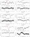 |
Fig. B.1 Plots of the light curves of the detected cometary transits in the first tier catalog. For each transit, the light curve is shown in the top panels over 5 days centered on the transit time and with an exocomet transit fit superimposed (red line). The bottom panels show the light curves over a larger time frame. |
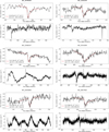 |
Fig. B.1 Continued |
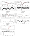 |
Fig. B.1 Continued |
Appendix C Possible exocometary transit light curves
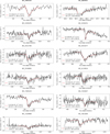 |
Fig. C.1 Plots of the light curves of the possibly detected cometary transits in the second tier catalog. The plots cover 5 days and are centered on the transit time and with an exocomet transit fit superimposed (red line). |
Appendix D Information on the stars of the second tier catalog
Information on the stars in the second tier catalog.
Appendix E Information on the stars of the third tier catalog
Third tier catalog of symmetric transits that could be either exocometary transits or exoplanet mono-transits.
All Tables
Third tier catalog of symmetric transits that could be either exocometary transits or exoplanet mono-transits.
All Figures
|
Fig. 1 Architecture of our best performing neural network model. The input data is a light curve of 480 timesteps, the output is a list of two real numbers between 0 and 1: one for the probability of detection of an exocometary transit and one for the position of the transit in the light curve. Convolutional layers are denoted Conv <kernel size> <number of feature maps>, max pooling layers are denoted MaxPool <window length> <stride length>, fully connected layers are denoted Dense <number of units>, LSTM layers are denoted LSTM <units> <dropout>, GRU layers are denoted GRU <unit> <droupout> <recurent dropout>, and the squeezed-excitation blocks are denoted SEB. |
| In the text | |
|
Fig. 2 Receiver-operator characteristic curve (left panel) and the precision vs. recall curve (right panel). The ROC curve shows the recall (true-positive rate) of the model against the ability to recognize false positives (false-positive rate) for different classification thresholds. Our model is highly successful at identifying false positives, as shown by the high AUC value (see Table A.1). The plot of the fraction of exocomets that the model classified as exocomets (recall) vs. the fraction of correctly classified planets (precision) shows the trade-off between having no false positives (high precision) and identifying all exocomet transits (high recall). |
| In the text | |
|
Fig. 3 Histogram of the results on the test set and error on the transit position found by the network. Top panel: histogram of the result of the neural network applied to the test data. Most of the 1-labeled light curves with an exocomet transit yield a probability close to 1, while there are only a few false positives (0-labeled light curves yielding a high probability). Above the chosen threshold, there is more than two order of magnitude between the number of true positives and false positive. Bottom panel: mean error of the position of the transit as a function of the probability of the presence of a transit assigned by the network to the light curves. This error is a few hours at most for the transits identified by the algorithm. |
| In the text | |
|
Fig. 4 Distribution of the value of the parameters obtained by fitting the 2163 light curves in the library of the simulated exocomet transits. The parameters K, ∆T = t1 − t0, and 1/β correspond to the depth, ingress duration, and crossing time of the transit, respectively. |
| In the text | |
|
Fig. B.1 Plots of the light curves of the detected cometary transits in the first tier catalog. For each transit, the light curve is shown in the top panels over 5 days centered on the transit time and with an exocomet transit fit superimposed (red line). The bottom panels show the light curves over a larger time frame. |
| In the text | |
|
Fig. B.1 Continued |
| In the text | |
|
Fig. B.1 Continued |
| In the text | |
|
Fig. C.1 Plots of the light curves of the possibly detected cometary transits in the second tier catalog. The plots cover 5 days and are centered on the transit time and with an exocomet transit fit superimposed (red line). |
| In the text | |
Current usage metrics show cumulative count of Article Views (full-text article views including HTML views, PDF and ePub downloads, according to the available data) and Abstracts Views on Vision4Press platform.
Data correspond to usage on the plateform after 2015. The current usage metrics is available 48-96 hours after online publication and is updated daily on week days.
Initial download of the metrics may take a while.