| Issue |
A&A
Volume 704, December 2025
|
|
|---|---|---|
| Article Number | L7 | |
| Number of page(s) | 13 | |
| Section | Letters to the Editor | |
| DOI | https://doi.org/10.1051/0004-6361/202556580 | |
| Published online | 09 December 2025 | |
Letter to the Editor
SVOM GRB 250314A at z ≃ 7.3: An exploding star in the era of re-ionization
1
CEA Paris-Saclay, Irfu/Département d’Astrophysique, 91191 Gif sur Yvette, France
2
National Astronomical Observatories, Chinese Academy of Sciences, Beijing 100101, China
3
School of Astronomy and Space Science, University of Chinese Academy of Sciences, Beijing 101408, China
4
School of Physics and Astronomy, University of Leicester, University Road, Leicester LE1 7RH, United Kingdom
5
UX, Observatoire de Paris, Université PSL, CNRS, Sorbonne Université, Meudon 92190, France
6
Sorbonne Université, CNRS, UMR 7095, Institut d’Astrophysique de Paris, 98 bis bd Arago, F-75014 Paris, France
7
Niels Bohr Institute, University of Copenhagen, Jagtvej 155, 2200 Copenhagen N, Denmark
8
The Cosmic Dawn Centre (DAWN), Denmark
9
Department of Astrophysics/IMAPP, Radboud University Nijmegen, P.O. Box 9010 Nijmegen 6500 GL, The Netherlands
10
Aix Marseille Univ., CNRS, CNES, LAM, Marseille, France
11
Université Paris-Saclay, Université Paris Cité, CEA, CNRS, AIM, 91191 Gif-sur-Yvette, France
12
IRAP, Université de Toulouse, CNRS, CNES, Toulouse, France
13
Department of Physics, University of Hong Kong, Pokfulam Road, Hong Kong, China
14
Nevada Center for Astrophysics and Department of Physics and Astronomy, University of Nevada, Las Vegas, NV 89154, USA
15
Key Laboratory of Particle Astrophysics, Institute of High Energy Physics, Chinese Academy of Sciences, Beijing 100049, China
16
Department of Astronomy, University of California, Berkeley, CA 94720-3411, USA
17
INAF, Istituto di Astrofisica e Planetologia Spaziali, Via Fosso del Cavaliere 100, Roma 00133, Italy
18
Department of Physics and Astronomy, Baylor University, One Bear Place #97316, Waco, TX 76798, USA
19
Department of Physics, University of Warwick, Coventry CV4 7AL, UK
20
School of Physics and Centre for Space Research, University College Dublin, Belfield, Dublin D04 V1W8, Ireland
21
Space Science Data Center (SSDC), Agenzia Spaziale Italiana (ASI), Roma I-00133, Italy
22
Centro Astronòmico Hispano en Andalucìa, Observatorio de Calar Alto, Sierra de los Filabres, Gèrgal, Almerìa 04550, Spain
23
Departament d’Astonomia i Astrofìsica, Universitat de València, C/Dr. Moliner, 50, E-46100 Burjassot (València), Spain
24
Obs. Astronòmic, Universitat de València, 46980 Paterna, Spain
25
National Space Science Center, Chinese Academy of Sciences, Beijing 100190, China
26
INAF – Osservatorio Astronomico di Brera, Via Bianchi 46, I-23807 Merate, LC, Italy
27
Laboratoire Univers et Particules de Montpellier, Université Montpellier, CNRS/IN2P3, F-34095 Montpellier, France
28
Astrophysics Research Institute, Liverpool John Moores University, Liverpool Science Park, 146 Brownlow Hill, Liverpool L3 5RF, United Kingdom
29
Astrophysics Science Division, NASA Goddard Space Flight Center, Mail Code 661, Greenbelt, MD 20771, USA
30
European Space Agency (ESA), European Space Research and Technology Centre (ESTEC), Keplerlaan 1, 2201 AZ Noordwijk, The Netherlands
31
Université Paris Cité, CNRS, Astroparticule et Cosmologie, F-75013 Paris, France
32
Centre National d’Etudes Spatiales, Centre Spatial de Toulouse, Toulouse Cedex 9, France
33
School of Physics and Astronomy, University of Birmingham, Edgbaston, Birmingham B15 2TT, UK
34
Aix Marseille Univ, CNRS/IN2P3, CPPM, Marseille, France
35
Institut d’Estudis Espacials de Catalunya (IEEC), E-08034 Barcelona, Spain
36
Institute of Space Sciences (ICE, CSIC), Campus UAB, Carrer de Can Magrans, s/n, E-08193 Barcelona, Spain
37
College of Science and Engineering, School of Mathematics and Physics, Kanazawa University, Kakuma, Kanazawa, 9201192 Ishikawa, Japan
38
Department of Astronomy, School of Physics, Huazhong University of Science and Technology, 1037 Luoyu Road, Wuhan 430074, PR China
39
Department of Physics & Astronomy, Clemson University, Clemson, SC 29634, USA
40
INAF, Osservatorio Astronomico di Capodimonte, Salita Moiariello 16, I-80121 Naples, Italy
41
DARK, Niels Bohr Institute, University of Copenhagen, Jagtvej 155A, 2200 Copenhagen, Denmark
42
Centre for Astrophysics and Cosmology, Science Institute, University of Iceland, Dunhagi 5, 107 Reykjavik, Iceland
43
Department of Astronomy and Astrophysics, Pennsylvania State University, 525 Davey Lab, University Park, PA 16802, USA
44
Department of Physics & Astronomy, University of Utah, Salt Lake City, UT 84112, USA
45
Key Lab for Satellite Digitalization Technology, Innovation Academy for Microsatellites, Chinese Academy of Sciences, No. 1 Xueyang Road, Shanghai 201304, China
46
Yunnan Observatories, Chinese Academy of Sciences, Kunming 650011, China
47
GRANTECAN S.A., Cuesta de San José s/n, E-38712 Breña Baja, La Palma, Spain
48
Instituto de Astrofísica de Canarias, E-38205 La Laguna, Tenerife, Spain
49
Royal Commission for AlUla, Riyadh, Saudi Arabia
50
Observatoire Astronomique de Strasbourg, Université de Strasbourg, CNRS, 11 rue de l’Université, F-67000 Strasbourg, France
51
Anton Pannekoek Institute of Astronomy, University of Amsterdam, P.O. Box 94249 1090 GE Amsterdam, The Netherlands
52
Université Paris-Saclay, CNRS/IN2P3, IJCLab, 91405 Orsay, France
53
Osservatorio di Astrofisica e Scienza dello Spazio, INAF, Via Piero Gobetti 93/3, Bologna 40129, Italy
54
INAF–Istituto di Astrofisica Spaziale e Fisica Cosmica di Milano, Via A. Corti 12, 20133 Milano, Italy
55
E. Kharadze Georgian National Astrophysical Observatory, Mt. Kanobili, Abastumani 0301, Adigeni, Georgia
56
Departmant of Physics, University of Bath, Claverton Down, Bath BA2 7AY, UK
57
Purple Mountain Observatory, Chinese Academy of Sciences, Nanjing 210023, China
⋆ Corresponding authors: This email address is being protected from spambots. You need JavaScript enabled to view it.
; This email address is being protected from spambots. You need JavaScript enabled to view it.
; This email address is being protected from spambots. You need JavaScript enabled to view it.
Received:
24
July
2025
Accepted:
28
September
2025
Abstract
Most long gamma-ray bursts (LGRBs) originate from a rare type of massive stellar explosion. Their afterglows, while rapidly fading, can initially be extremely luminous at optical and near-infrared wavelengths, making them detectable at large cosmological distances. Here we report the detection and observations of GRB 250314A by the SVOM satellite and the subsequent follow-up campaign that led to the discovery of the near-infrared afterglow and spectroscopic measurements of its redshift z ≃ 7.3. This burst occurred when the Universe was only about 5% of its current age. We discuss the signature of these rare events within the context of the SVOM operating model and the ways to optimise their identification with adapted ground follow-up observation strategies.
Key words: gamma-ray burst: general / galaxies: high-redshift / gamma-ray burst: individual: GRB250314A
© The Authors 2025
 Open Access article, published by EDP Sciences, under the terms of the Creative Commons Attribution License (https://creativecommons.org/licenses/by/4.0), which permits unrestricted use, distribution, and reproduction in any medium, provided the original work is properly cited.
This article is published in open access under the Subscribe to Open model. This email address is being protected from spambots. You need JavaScript enabled to view it. to support open access publication.
1. Introduction
Long gamma-ray bursts (LGRBs) have long been regarded as powerful tools for exploring the early Universe. Originating from the explosion of rare massive stars (Hjorth et al. 2003, 2012; Woosley & Bloom 2006; Cano et al. 2017), they produce intense afterglow emission that can be detected up to the highest redshifts, for example z ∼ 10, and beyond (Kann et al. 2024). Their direct association with individual stars makes them key tracers of star formation (e.g. Krogager et al. 2024), including when their host galaxies are too faint to be observed directly through emission lines, even with sensitive facilities such as the James Webb Space Telescope (JWST). With multiple gamma-ray bursts (GRBs) detected at z > 6, we could begin probing the high-redshift Universe and chemically characterise their host interstellar medium (ISM) thanks to GRB afterglow spectroscopy (Hartoog et al. 2015; Saccardi et al. 2023, 2025). Furthermore, precise analysis of the Lyman-α break could allow an estimation of the neutral hydrogen column density of the GRB host galaxy (Tanvir et al. 2019). The new identification of distant events is therefore highly desirable. However, to date, we are statistically limited by a small number of GRBs at very high redshift (z > 7), and only two have a well-constrained spectroscopic redshift, with a low signal-to-noise spectrum without identification of metal absorption lines, zspec = 8.23 (GRB 090423A; Salvaterra et al. 2009; Tanvir et al. 2009) and zspec = 7.8 (GRB 120923A; Tanvir et al. 2018). Other high-redshift GRBs have been discovered, but only a photometric redshift has been derived: zphot ≃ 9.4 (GRB 090429B; Cucchiara et al. 2011) and zphot ≃ 7.88 (GRB 100905A; Bolmer et al. 2018). Given the rarity of these high-redshift events and the faintness of such sources, the scientific outcome is strongly dependent on the responsiveness of the follow-up activities.
The new satellite SVOM (Space-based multi-band astronomical Variable Objects Monitor; Wei et al. 2016), a Sino-French mission of CNSA (China National Space Administration) and CNES (Centre National d’Études Spatiales) launched on 22 June 2024, has been designed to favour the detection andcharacterisation of high-redshift GRBs (Cordier et al. 2008). For this purpose, the SVOM collaboration has developed dedicated partnerships with other space- and ground-based facilities. In this Letter we present the first result of this effort: the SVOM detection of GRB 250314A at z ≃ 7.3 and the subsequent follow-up of its afterglow. In a companion paper, Levan et al. (2025) report JWST observations that likely provide direct evidence for the association of this GRB with a massive star progenitor. All errors are given at the 68% confidence level when not stated otherwise.
2. Observations, data analysis, and results
Detection, localisation, and slew. On 14 March 2025, the SVOM/ECLAIRs coded-mask telescope (Godet et al. 2014) automatically detected and localised GRB 250314A starting at 12:56:42 UTC (Tb), hereafter used as the time reference. Four alert packets were produced and transmitted immediately to the ground thanks to the SVOM very high frequency (VHF) network (see Appendix A.1). As detailed in Appendix A.2, the first alert reports an excess detected over an interval of 10.24 s in the 8–50 keV energy band starting at Tb. The localisation of the best alert was at RA = 201.272°, Dec = −5.293° (J2000) with a 90% confidence level radius of 8.62 arcmin, including a 2 arcmin systematic error added in quadrature (Wang et al. 2025). The trigger requested the spacecraft slew at Tb+43 s, effectively locating GRB 250314A in the centre of the field of view of the four SVOM instruments.
Prompt GRB observations. GRB 250314A was detected by both gamma-ray instruments on board SVOM, ECLAIRs, and the Gamma Ray Monitor (GRM; Dong et al. 2010; He et al. 2025). Their data analysis is detailed in Appendix B. In the light curves shown in Fig. 1, GRB 250314A appears as a weak single pulse burst, with a T90 duration of  s in 4–100 keV (ECLAIRs) and 7.50
 s in 15–5000 keV (GRM). The analysis of the spectrum leads to a time-averaged flux of 5.1
 in 4–120 keV (ECLAIRs) and 3.27
 in 15–5000 keV (GRM). The joint spectral analysis of ECLAIRs+GRM data shows that the time-averaged spectrum is best fitted by a power law with an exponential cut-off (Fig. B.2), with a photon index of
  and a peak energy of
  keV.
keV.
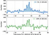 |
Fig. 1. Background subtracted light curves for ECLAIRs in the4–100 keV energy range (top panel) and for GRM in the 15–300 keV energy range (bottom panel) using a time bin of 1 s. |
X-ray follow-up with SVOM/MXT, Swift/XRT and EP/FXT: afterglow detection. Following the slew of the satellite, the Microchannel X-ray Telescope (MXT; Götz et al. 2023) on board SVOM began observing the field of GRB 250314A at Tb+177 s. The MXT observation lasted until 16:18:49 UT accumulating an effective exposure time of 4950 s on source, due to Earth occultations, South Atlantic Anomaly (SAA) passages, and stray-light limitations. The analysis of MXT data is detailed in Appendix C. The afterglow of GRB 250314A was not detected. The first kilosecond of the observation led to a 3σ upper limit of 2.5 × 10⁻¹¹ erg cm−2 s−1 in the 0.3–10 keV energy band. To complement the MXT observations, we requested several target-of-opportunity (ToO) follow-up observations using both the Neil Gehrels Swift Observatory/XRT (Burrows et al. 2005) and the Einstein Probe/FXT (Chen et al. 2020) X-ray telescopes (0.3–10 keV). As reported in Appendix C.2, an uncatalogued fading X-ray source in the first Swift/XRT (Kennea et al. 2025) and EP/FXT (Turpin et al. 2025) observations was clearly detected at an enhanced Swift/XRT position RA = 13h 25m 12.33s and Dec = −05° 16′56.1″ (J2000) with an uncertainty of 3.4″. As this new X-ray transient has a position consistent with that of the ECLAIRs GRB and shows a clear fading signature, we confidently identify it as the X-ray afterglow of GRB 250314A. The spectral analysis of Swift/XRT and EP/FXT data is detailed in Appendix C. In all cases the best spectral fit was obtained by an absorbed power law (photon index ∼ 2.4) whose fitted NH value is compatible with values exceeding the Galactic value (2.46 × 1020 cm−2, HI4PI Collaboration 2016); see discussion in Appendix C. The derived fluxes of our observations are given in Table C.1 and lead to the light curve shown in the top panel of Fig. C.1, where it is compared to a sample of other high-z afterglows. We notice that the flaring activity shown by several high-z afterglows detected in the past is clearly excluded by our early time MXT observations.
X-ray follow-up observations.
Follow-up with SVOM/VT. Following the slew, the Visible Telescope (VT; Fan et al. 2020) on board SVOM began the follow-up of the field at Tb+186 s in the VT_B (400–650 nm) and VT_R (650–1000 nm) channels simultaneously. The follow-up lasted for three orbits. As detailed in Appendix D, no uncatalogued sources brighter than 20 mag were found within the ECLAIRs error region from the quick-look analysis of the VHF data (Palmerio et al. 2025). The stacking of the complete image dataset received later revealed no candidate within the Swift/XRT error box and resulted in a 3σ upper limits of 23.5 mag in VT_B and 23.0 mag in VT_R band at 13.9 minutes after Tb (see Table D.1). These early VT deep optical upper limits suggest a potential high-redshift (z > 6) candidate (Li et al. 2025).
Ground-based follow-up observations with the NOT, the VLT and the GTC: afterglow detection and redshift measurement. We triggered the Nordic Optical Telescope (NOT) as soon as the X-ray localisation became available. Imaging in the J band was secured with the near-infrared (NIR) camera NOTCam (FoV: 4′×4′), beginning 12.1 h after Tb. Consistent with the Swift/XRT and EP/FXT X-ray localisation, a single object was detected, not visible in archival images of this field at RA = 13h 25m 12.16s and Dec = −05° 16′55.1″ with an uncertainty of 0.1″ (Malesani et al. 2025). A second NOTCam observation was performed the following night, only yielding an upper limit to the target brightness. Following the identification of the counterpart, we initiated within the ‘Stargate’ programme a photometric and spectroscopic follow-up at the ESO Very LargeTelescope (VLT), using the High Acuity Wide field K-band Imager (HAWK-I) in the YJH filters and with the X-shooter spectrograph (Vernet et al. 2011). HAWK-I observations began 16.45 h after Tb. The afterglow was detected in all of the filters, clearly fading compared to the NOT measurement, thereby identifying this object as the afterglow of GRB 250314A. Photometry was also secured 16.81 h after Tb at the 10.4-m Gran Telescopio Canarias (GTC) telescope, using the OSIRIS+ instrument and the z filter. This served as a ‘veto’ filter, expecting a deep non-detection in the optical band due to the source spectrum drop-out. The data reduction is detailed in Appendix E, and all magnitudes are reported in Table E.1. These data produce the light curve in the bottom panel of Fig. C.1, where it is compared to the available sample of high-z GRBs. X-shooter observations began 16.62 h after Tb. The spectra cover the wavelength range 3000–21 000 Å and the spectral analysis is detailed in Appendix E. The spectrum shown in Fig. 2 reveals a flat spectral continuum that sharply drops off below λ ∼ 10090 Å, consistent with a Lyman-α break caused by absorption from neutral hydrogen, as shown in Fig. 2 (Right). Despite the low signal-to-noise ratio, fitting this feature unambiguously indicates a redshift of z ≃ 7.3. The details of the fit and the full corner plots of the parameters are shown in Fig. E.1. Unfortunately, no individual metal absorption features have been confidentially identified (see the discussion on equivalent width (EW) upper limits in Appendix E).
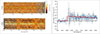 |
Fig. 2. Left: 2D VIS (top) and NIR (bottom) VLT/X-shooter spectra. The VIS spectrum is cut at 8000 Å, and the vertical dashed black line marks the position corresponding to the Ly-α observer frame wavelength at z ≃ 7.3. Right: 1D re-binned combined spectrum from 9000 to 13 000 Å. The solid red line shows the best fitting afterglow model (Appendix E). Note that the increased noise around the break location is an unfortunate consequence of it being close to the boundary between the VIS and NIR arms. |
Radio follow-up campaign. The determination of the redshift triggered a radio follow-up campaign. The radio afterglow is detected by VLA at 6.7 days (Nayana et al. 2025) and ATCA at 8.96 days. ALMA observations at 11.6 days after Tb led to the most precise localisation (Laskar et al. 2025). Data acquired with ATCA, e-MERLIN, MeerKAT, and VLA from 6.7 to 109 days after Tb are presented and discussed in Appendix F.
3. Discussion and conclusions
Our observations, triggered by the detection of GRB250314A on board SVOM (timeline discussed in Appendix G), led to the identification of a new GRB above z = 7. We summarise below the results that lead us to associate this GRB to a massive star progenitor, complementary to the possible direct evidence provided by JWST observations presented in Levan et al. (2025). This confirms the importance of GRBs as probes of star formation in the early Universe and and leads us to discuss how the follow-up strategy may still be optimised to enlarge the high-z GRB sample.
3.1. Classification of GRB 250314A.
As discussed in Appendix H, the rest-frame peak energy  keV and isotropic-equivalent energy
  in the 10 keV–10 MeV energy range of GRB 250314A are consistent with a classification as a ‘long’ GRB (type II): see Fig. H.1. The rather short T90 duration in the burst rest frame (
 ) is probably due to a ‘tip of the iceberg effect’ considering the weakness of this GRB (Llamas Lanza et al. 2024), which is also often observed in other high redshift GRBs (see discussion in Appendix B.2). As seen in Fig. H.1, the properties of GRB 250314A are not extreme, although its isotropic equivalent energy lies in the bright half of the sample, similar to other high redshift GRBs. We conclude that GRB 250314A appears as a classical long (type II) GRB, most probably associated with a massive star progenitor (see e.g. discussion in Li et al. 2020). The low-energy threshold of ECLAIRs at 4 keV favours the detection of such high-redshift GRBs (Palmerio & Daigne 2021). However, their early identification remains a challenge and requires a specific strategy.
3.2. Optimising SVOM follow-up strategy for high-z GRBs
An important goal of the SVOM mission is to increase the fraction of GRBs with redshift determinations, aiming to increase the low number of identified high-z GRBs to date (12 GRBs at z > 6) and to use them as probes of stars and galaxies in the early Universe, up to the re-ionisation era. To reach these goals, two key factors are necessary: a rapid determination of the precise afterglow position, and the availability of sensitive optical-NIR spectrographs. To this aim, SVOM benefits from two major assets: the slew capability, allowing the fast repointing (< 2 min) of the on-board instruments MXT and VT, and the VT sensitivity and spectral coverage including the reddest part of the optical domain. Furthermore, for the follow-up of the GRB afterglows, the SVOM mission also includes dedicated ground-based facilities to perform real-time photometry. In addition, the SVOM team has established agreements with the Swift and EP teams to obtain additional rapid X-ray follow-up observations, as well as with several collaborations with access to large ground-based telescopes for deep photometry and spectroscopy.
From its launch up to 12 July 2025, the VT automatically followed up 26 ECLAIRs-triggered GRBs1, with a delay of several minutes after the trigger, detecting the optical counterpart of 19 of these (73%). By performing a rapid analysis of VHF data (Appendix D), initial results identifying bright candidates can be distributed within an hour. More precise and deeper detection results can be obtained using X-band data, which are typically obtained within 5–7 hours (Appendix A.1). The precise localisations of the X-ray afterglow help us draw more firm conclusions, especially in cases where no optical detection is available. This has already led to 14 redshift determinations (54%). Of the seven GRBs without optical afterglow detection, one was affected by the strong stray light from Earth during the early phase, which limited the detection ability (Qiu et al. 2025). Three of them may be caused by heavy extinction, as indicated by the relatively high excess column density deduced from the X-ray afterglow spectrum (Evans et al. 2025; Osborne et al. 2025). GRB 250314A is one of the remaining three. The other two (GRB 250507A and GRB 250127A) are also high-redshift GRB candidates, even though high-extinction or optically faint GRBs cannot be excluded.
The follow-up of very high-redshift (z > 6) GRB candidates represents an additional challenge. There are few NIR facilities capable of ToO observations soon after a GRB detection. As they have limited time allocated for afterglow observations, preliminary indications of a possible high-redshift GRB origin are necessary to activate such observations. Therefore, obtaining early-time VT deep limits on the afterglow magnitude is extremely important, and an X-ray afterglow position with an accuracy better than 10″ is essential to reduce the ECLAIRs or MXT error box and filter out potential contaminants. Both factors played a key role in the discovery of GRB 250314A. This event also highlights the importance of setting up efficient coordination and communication between SVOM and follow-up collaborations. The timeline in Fig. H.2 indicates a period of approximately 17 hours between the ECLAIRs trigger and the start of the VLT observation. This delay is due to the availability of two key pieces of information: the X-ray location and the deep VT upper limits. They arrived late, 11 hours and 15 hours, respectively, after the trigger, whereas the corresponding observations were completed much earlier. The delay in determining the X-ray localisation is notably long due to data transmission gaps. The usual delay is approximately 3 hours. The delay in determining deep limits from the VT data is clearly a weakness that requires improvement.
In conclusion, the observations of GRB 250314A presented in this Letter allow us to include one more GRB in the small sample at z > 7 and to identify the key factors that still limit the identification of such high-redshift GRBs. In the future, we stress that a game-changing GRB mission capable of autonomously localising and performing spectroscopy of high-redshift GRBs would be transformative. In the short term, significant progress is still expected with SVOM: (i) To make VT deep optical early-time upper limits available earlier than for GRB 250314A, the main goal will be to increase the number of X-band stations to recover the full telemetry more rapidly. Once the precise X-ray localisation and the VT X-band data are available, the automation of VT data analysis can further improve the rapid dissemination of crucial results, facilitating NIR follow-up trigger. (ii) The NIR follow-up will benefit from new facilities, including the start of the SOXS spectrograph (Schipani et al. 2018) operations in 2026 and the commissioning of the CAGIRE camera (Fortin et al. 2024) at the Colibrí telescope focus in June 2026. This represents a considerable addition to the handful of NIR instruments available to date for GRB follow-up, especially because both instruments are specifically meant for the follow-up of transient phenomena. Specific agreements guarantee that both instruments will have dedicated follow-up time for all SVOM GRBs observable from the San Pedro Mártir and ESO/La Silla observatories, respectively, as soon as they are visible (CAGIRE) and once a relatively precise (less than ∼2′) localisation is available (SOXS). CAGIRE will be less sensitive than HAWK-I (J ∼ 19 in 5 minutes of observations). However, its availability for SVOM triggers, field of view, and simultaneous observations with the optical instruments on Colibrí will improve the chances of identifying high-redshift GRB afterglows, particularly in their early phases, and will help determine their precise localisation. While SOXS is not as performant as X-shooter in terms of sensitivity and resolution, it will provide a step forward in obtaining afterglow spectroscopy of high-redshift GRBs. In fact, to date, spectroscopy of GRBs at z > 6 has relied on X-shooter availability, which remains the only spectrograph suitable for such observations.
This optimised follow-up strategy will be key to obtaining NIR spectroscopy at earlier times than for GRB 250314A, enabling high signal-to-noise ratio (S/N) spectra and fully exploiting the possibility to probe high-redshift galaxies and re-ionisation with GRBs.
This represents only about 60% of ECLAIRs-triggered GRBs as the automatic slew was only gradually enabled a few months later.
The abundances used are from Anders & Grevesse (1989)
References
- Amati, L., Frontera, F., Tavani, M., et al. 2002, A&A, 390, 81 [NASA ADS] [CrossRef] [EDP Sciences] [Google Scholar]
- Anders, E., & Grevesse, N. 1989, Geochim. Cosmochim. Acta, 53, 197 [Google Scholar]
- Atteia, J.-L., Bouchet, L., Dezalay, J.-P., et al. 2025, ApJ, 980, 241 [Google Scholar]
- Bolmer, J., Greiner, J., Krühler, T., et al. 2018, A&A, 609, A62 [NASA ADS] [CrossRef] [EDP Sciences] [Google Scholar]
- Brivio, R., Campana, S., Covino, S., et al. 2025, A&A, 695, A239 [NASA ADS] [CrossRef] [EDP Sciences] [Google Scholar]
- Burrows, D. N., Hill, J. E., Nousek, J. A., et al. 2005, Space Sci. Rev., 120, 165 [Google Scholar]
- Cano, Z., Wang, S.-Q., Dai, Z.-G., & Wu, X.-F. 2017, Adv. Astron., 2017, 8929054 [CrossRef] [Google Scholar]
- Cash, W. 1979, ApJ, 228, 939 [Google Scholar]
- Chandra, P., & Frail, D. A. 2012, ApJ, 746, 156 [NASA ADS] [CrossRef] [Google Scholar]
- Chen, Y., Cui, W., Han, D., et al. 2020, SPIE Conf. Ser., 11444, 114445B [Google Scholar]
- Cordier, B., Desclaux, F., Foliard, J., & Schanne, S. 2008, AIP Conf. Ser., 1000, 585 [Google Scholar]
- Cucchiara, A., Levan, A. J., Fox, D. B., et al. 2011, ApJ, 736, 7 [Google Scholar]
- de Ugarte Postigo, A., Fynbo, J. P. U., Thöne, C. C., et al. 2012, A&A, 548, A11 [NASA ADS] [CrossRef] [EDP Sciences] [Google Scholar]
- de Ugarte Postigo, A., Thöne, C. C., Bensch, K., et al. 2018, A&A, 620, A190 [NASA ADS] [CrossRef] [EDP Sciences] [Google Scholar]
- Dong, Y., Wu, B., Li, Y., Zhang, Y., & Zhang, S. 2010, Sci. China: Phys. Mech. Astron., 53, 40 [Google Scholar]
- Evans, P. A., Willingale, R., Osborne, J. P., et al. 2010, A&A, 519, A102 [NASA ADS] [CrossRef] [EDP Sciences] [Google Scholar]
- Evans, P. A., Kennea, J. A., Ambrosi, E., et al. 2025, GCN, 40579 [Google Scholar]
- Fan, X., Zou, G., Wei, J., et al. 2020, SPIE Conf. Ser., 11443, 114430Q [Google Scholar]
- Fortin, F., Atteia, J. L., Nouvel de la Flèche, A., et al. 2024, A&A, 691, A324 [NASA ADS] [CrossRef] [EDP Sciences] [Google Scholar]
- Frail, D. A., Berger, E., Galama, T., et al. 2000, ApJ, 538, L129 [NASA ADS] [CrossRef] [Google Scholar]
- Godet, O., Nasser, G., Atteia, J., et al. 2014, SPIE Conf. Ser., 9144 [Google Scholar]
- Gorbovskoy, E. S., Lipunova, G. V., Lipunov, V. M., et al. 2012, MNRAS, 421, 1874 [NASA ADS] [CrossRef] [Google Scholar]
- Götz, D., Boutelier, M., Burwitz, V., et al. 2023, Exp. Astron., 55, 487 [CrossRef] [Google Scholar]
- Hartoog, O. E., Malesani, D., Fynbo, J. P. U., et al. 2015, A&A, 580, A139 [NASA ADS] [CrossRef] [EDP Sciences] [Google Scholar]
- He, J., Sun, J.-C., Dong, Y.-W., et al. 2025, Exp. Astron., 59, 15 [Google Scholar]
- HI4PI Collaboration (Ben Bekhti, N., et al.) 2016, A&A, 594, A116 [NASA ADS] [CrossRef] [EDP Sciences] [Google Scholar]
- Hjorth, J., Sollerman, J., Møller, P., et al. 2003, Nature, 423, 847 [Google Scholar]
- Hjorth, J., Malesani, D., Jakobsson, P., et al. 2012, ApJ, 756, 187 [Google Scholar]
- Kann, D. A., Klose, S., Zhang, B., et al. 2010, ApJ, 720, 1513 [Google Scholar]
- Kann, D. A., White, N. E., Ghirlanda, G., et al. 2024, A&A, 686, A56 [NASA ADS] [CrossRef] [EDP Sciences] [Google Scholar]
- Kennea, J. A., D’Elia, V., Evans, P. A., & Swift/XRT Team 2025, GCN, 39734 [Google Scholar]
- Krogager, J. K., De Cia, A., Heintz, K. E., et al. 2024, MNRAS, 535, 561 [Google Scholar]
- Lan, L., Gao, H., Li, A., et al. 2023, ApJ, 949, L4 [Google Scholar]
- Laskar, T., van Eerten, H., Schady, P., et al. 2019, ApJ, 884, 121 [NASA ADS] [CrossRef] [Google Scholar]
- Laskar, T., Margutti, R., Chornock, R., et al. 2025, GCN, 40012 [Google Scholar]
- Levan, A. J., Schneider, B., Le Floc’h, E., et al. 2025, A&A, 704, L8 [NASA ADS] [CrossRef] [EDP Sciences] [Google Scholar]
- Li, Y., Zhang, B., & Yuan, Q. 2020, ApJ, 897, 154 [NASA ADS] [CrossRef] [Google Scholar]
- Li, H. L., Li, R. Z., Wang, Y., et al. 2025, GCN, 39728 [Google Scholar]
- Lien, A., Sakamoto, T., Barthelmy, S. D., et al. 2016, ApJ, 829, 7 [Google Scholar]
- Littlejohns, O. M., Tanvir, N. R., Willingale, R., et al. 2013, MNRAS, 436, 3640 [NASA ADS] [CrossRef] [Google Scholar]
- Llamas Lanza, M., Godet, O., Arcier, B., et al. 2024, A&A, 685, A163 [NASA ADS] [CrossRef] [EDP Sciences] [Google Scholar]
- Lü, H.-J., Zhang, B., Liang, E.-W., Zhang, B.-B., & Sakamoto, T. 2014, MNRAS, 442, 1922 [Google Scholar]
- Malesani, D. B., Corcoran, G., Izzo, L., et al. 2025, GCN, 39727 [Google Scholar]
- McMahon, R. G., Banerji, M., Gonzalez, E., et al. 2021, VizieR On-line Data Catalog: II/367 [Google Scholar]
- McMullin, J. P., Waters, B., Schiebel, D., Young, W., & Golap, K. 2007, ASP Conf. Ser., 376, 127 [Google Scholar]
- Modigliani, A., Goldoni, P., Royer, F., et al. 2010, Proc. SPIE, 7737 [Google Scholar]
- Moldon, J. 2021, Astrophysics Source Code Library [record ascl:2109.006] [Google Scholar]
- Moss, M., Lien, A., Guiriec, S., Cenko, S. B., & Sakamoto, T. 2022, ApJ, 927, 157 [NASA ADS] [CrossRef] [Google Scholar]
- Nayana, A., Jr., Laskar, T., Margutti, R., et al. 2025, GCN, 39954 [Google Scholar]
- Osborne, J. P., D’Avanzo, P., Bernardini, M. G., et al. 2025, GCN, 38918, 1 [Google Scholar]
- Palmerio, J. T., & Daigne, F. 2021, A&A, 649, A166 [NASA ADS] [CrossRef] [EDP Sciences] [Google Scholar]
- Palmerio, J. T., Xin, L. P., Vergani, S. D., et al. 2025, GCN, 39722 [Google Scholar]
- Pei, Y. C. 1992, ApJ, 395, 130 [Google Scholar]
- Planck Collaboration VI. 2020, A&A, 641, A6 [NASA ADS] [CrossRef] [EDP Sciences] [Google Scholar]
- Qiu, Y. L., Li, H. L., Liang, Y. F., et al. 2025, GCN, 38824 [Google Scholar]
- Rossi, A., Frederiks, D. D., Kann, D. A., et al. 2022, A&A, 665, A125 [NASA ADS] [CrossRef] [EDP Sciences] [Google Scholar]
- Saccardi, A., Vergani, S. D., De Cia, A., et al. 2023, A&A, 671, A84 [NASA ADS] [CrossRef] [EDP Sciences] [Google Scholar]
- Saccardi, A., Vergani, S. D., Izzo, L., et al. 2025, A&A, submitted [arXiv:2506.04340] [Google Scholar]
- Salvaterra, R., Della Valle, M., Campana, S., et al. 2009, Nature, 461, 1258 [NASA ADS] [CrossRef] [PubMed] [Google Scholar]
- Schanne, S., Dagoneau, N., Château, F., et al. 2019, Mem. Soc. Astron. It., 90, 267 [Google Scholar]
- Schipani, P., Campana, S., Claudi, R., et al. 2018, SPIE Conf. Ser., 10702, 107020F [Google Scholar]
- Schlafly, E. F., & Finkbeiner, D. P. 2011, ApJ, 737, 103 [Google Scholar]
- Selsing, J., Malesani, D., Goldoni, P., et al. 2019, A&A, 623, A92 [NASA ADS] [CrossRef] [EDP Sciences] [Google Scholar]
- Starling, R. L. C., Willingale, R., Tanvir, N. R., et al. 2013, MNRAS, 431, 3159 [Google Scholar]
- Tanvir, N. R., Fox, D. B., Levan, A. J., et al. 2009, Nature, 461, 1254 [Google Scholar]
- Tanvir, N. R., Levan, A. J., Fruchter, A. S., et al. 2012, ApJ, 754, 46 [Google Scholar]
- Tanvir, N. R., Laskar, T., Levan, A. J., et al. 2018, ApJ, 865, 107 [NASA ADS] [CrossRef] [Google Scholar]
- Tanvir, N. R., Fynbo, J. P. U., de Ugarte Postigo, A., et al. 2019, MNRAS, 483, 5380 [Google Scholar]
- Turpin, D., Cordier, B., Cheng, H. Q., et al. 2025, GCN, 39739 [Google Scholar]
- Vernet, J., Dekker, H., D’Odorico, S., et al. 2011, A&A, 536, A105 [NASA ADS] [CrossRef] [EDP Sciences] [Google Scholar]
- Wang, Y., Li, R.-Z., Brunet, M., et al. 2025, GCN, 39719 [Google Scholar]
- Wei, J., Cordier, B., Antier, S., et al. 2016, arXiv eprints [arXiv:1610.06892] [Google Scholar]
- Woosley, S. E., & Bloom, J. S. 2006, ARA&A, 44, 507 [Google Scholar]
- Yasuda, T., Urata, Y., Enomoto, J., & Tashiro, M. S. 2017, MNRAS, 466, 4558 [Google Scholar]
Appendix A: Trigger, first localisation, and data transmission
A.1. Data transmission: VHF and X band data
SVOM data are received on ground via two different channels: (i) selected data can be transmitted in near-real time via a VHF network (hereafter ‘VHF data’); (ii) complete data are transmitted with a delay of a few hours, depending on the frequency with which X-band stations are available for the SVOM mission (hereafter ‘X-band data’). During the sequence following an on-board trigger, VHF data include alert packets (Appendix A.2) and selected data which are both generated by the on-board processing pipelines and used for the quick-look analysis on-ground. In case of a slew of the spacecraft, VHF data include an early photon list for the MXT, and source lists and 1-bit images for the VT, both around the ECLAIRs localisation. X-band data include event-by-event data from ECLAIRs and GRM and all images obtained by MXT and VT, and are processed on-ground. In the case of GRB 250314A, MXT and VT VHF data were received 15 min and 49 min after the ECLAIRs trigger respectively, and X-band data were received with a delay of 4.7 hours.
A.2. ECLAIR on-board trigger and localisation
The SVOM/ECLAIRs onboard trigger automatically detected and localised GRB 250314A and produced 4 different VHF alerts packets, sent to the onboard VHF emitter. The first VHF alert was produced at 12:56:58 UTC (T0) and covered the observation starting at 12:56:42 (Tb) over 10.24 s in the 8–50 keV energy band. The second VHF alert covered the same time range in the 8–120 keV band and provided the best localisation, reported in Sect. 2, with a maximum S/N of 9.18 σ (4.41 σ above noise). The localisations of all four alerts were consistent (Fig. A.1). Those alerts were produced by the Count-Rate Trigger (CRT), an algorithm which searches for time periods with detector-count excesses over background, followed by the reconstruction of their sky image, in which a new and uncatalogued source is searched for (Schanne et al. 2019). The trigger requested the spacecraft slew at T0+27 s and terminated the alert sequence 6 s later after confirmation of the slew start. It also sent VHF light-curve and VHF shadow-gram packets, containing the detector plane image of the best alert (Fig. A.2).
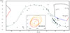 |
Fig. A.1. Location of the burst on the sky in Galactic coordinates (red point). The four alert packets produced by the trigger (inset) have coherent source positions, located well inside the 90 % c.l. error ellipses. |
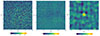 |
Fig. A.2. SVOM/ECLAIRs VHF shadow-gram (left) showing the number of counts per detector plane pixel during the time period of the best alert. De-convolved full-sky image (middle) is expressed in units of S/N (σ). A zoom-in on the detected source in the sky image is shown on the right. |
Appendix B: ECLAIRs and GRM data analysis
B.1. GRM detection
Since GRB 250314A triggered ECLAIRs first, GRM followed with an observation sequence driven by ECLAIRs. The analysis of the GRM X-band data shows a clear detection consistent with the ECLAIRs one, with high S/N in a timescale of 2 s.
B.2. Light curve and duration
Most of the burst emission in ECLAIRs is detected between 4 and 100 keV. The background-subtracted light-curve in Fig. 1 (top) was built during the analysis of X-band data by selecting only pixels of the detection plane illuminated by the burst over a specific time window from Tb-109 s to Tb+65 s. This approach effectively minimises background noise, thereby enhancing the accuracy of the background-subtracted light curves and facilitating a more precise estimation of the event duration. The background-subtracted light-curve obtained from the analysis of GRM X-band data (Fig. 1, bottom) also consists of a single pulse. The T90 durations reported in Sect. 2 were determined by calculating the median of their distributions. These distributions were generated through simulations that employed Poisson resampling of the observed light curves.
The result  s in the 4–100 keV band of ECLAIRs corresponds to a rather short T90 duration in the burst rest frame (
 ). The measured duration is however very sensitive to the energy range and sensitivity of the detector, and the burstS/N (see e.g. the discussion for Swift/BAT in Moss et al. 2022). Such short durations are observed in most GRBs above z = 7 as shown in Fig. B.1 and can be interpreted as a ‘tip of the iceberg effect’, as discussed in Littlejohns et al. (2013), Lü et al. (2014). Such an effect is also expected for high redshift GRBs detected by ECLAIRs as shown in the pre-launch simulations performed by Llamas Lanza et al. (2024) (see their Fig. 3).
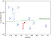 |
Fig. B.1. Observed T90 duration as a function of the redshift for the current sample of GRBs above z ∼ 6. The observed T90 duration in 4–100 keV of GRB 250314A is shown in red. The observed T90 durations in 15–150 keV of the other bursts in blue are taken from the Swift/BAT catalogue (Lien et al. 2016). The dotted green line corresponds to a duration of 2 s in the burst rest frame. |
B.3. Spectral analysis
The best time interval to build the spectrum of GRB 250314A was found using reconstructed ECLAIRs sky images over different time intervals so that the source was detected with S/N larger than 3. This leads to an interval of 11 s from Tb-1 s to Tb+10 s, used for the analysis of the time-averaged spectrum by ECLAIRs, GRM and ECLAIRs+GRM.
ECLAIRs spectral analysis. We extracted the time-averaged spectrum using the ECLAIRs pipeline (ECPI) version 1.18.0. ECPI first produces Good Time Intervals (GTIs) by filtering auxiliary and housekeeping data (i.e. filtering out satellite passages through the SAA, excluding time intervals when the satellite pointing is unstable, and selecting data according to Earth occultation conditions). The pipeline discards all events exhibiting abnormal Pulse Height Analyser (PHA) values, each event being identified by its pixel position and associated energy channel. Then, the event energy is calculated using a linear calibration function that accounts for the pixel-specific gain and offset parameters and is assigned to a unique Pulse Invariant (PI) channel. ECPI corrects detector images produced in different energy bands for efficiency, non-uniformity, and Earth occultation. From these corrected detector images, the pipeline applies a deconvolution procedure to reconstruct sky images and performs coding noise cleaning.
In addition, based to the burst position in these sky images, the pipeline builds a specific shadow-gram model. The shadow-gram model is fitted to the detector maps to extract the flux information for each energy bin. A second-degree polynomial is used to account for the background component. The response matrix file ECL-RSP-RMF_20220515T103600.fits and the ancillary response file ECL-RSP-ARF_20220515T104100.fits were used in the analysis. The ECLAIRs time-averaged spectrum is best fitted (χ2/d.o.f. = 19/21) in the 5–100 keV band by a power-law with a photon index of 1.2 ± 0.1 corresponding to a 4–120 keV time-averaged flux of 5.1 .
.
GRM spectral analysis. We used all three Gamma-Ray Detectors (GRDs) to extract the time-averaged spectrum. The Earth atmosphere albedo is not taken into account in the responses as the orientation of the three GRDs are all away from the Earth, and the flux of the burst is relatively low. The GRM time-averaged spectrum is best-fitted by a cut-off power-law model (CPL), with parameters of  and
and  keV (stat/d.o.f.∼34/24). This corresponds to a time-averaged flux of 3.27
 in the 15-5000 keV band.
ECLAIRs+GRM joint spectral analysis. We then performed a joint spectral analysis in the 5 keV–5 MeV energy band. The time-averaged spectrum is best fitted by a CPL model with a photon index  , a peak energy
  keV and a normalisation
  ph cm−2 s−1 keV−1 at 1 keV (stat/d.o.f. = 152/147). The posterior distributions of the model parameters are shown in Fig. B.2. Note that given the burst weakness the peak energy is not well constrained.
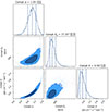 |
Fig. B.2. Best-fit parameters of the ECLAIRs and GRM joint spectral fits using a CPL model in the 5 keV – 5 MeV energy band. Errors are quoted at the 1 σ level. |
Appendix C: X-ray data analysis
C.1. SVOM/MXT data analysis
MXT data were acquired in the standard event mode and processed with the MXT pipeline v1.12. The MXT on board software, attempting localisations on increasingly longer exposure times, starting from 30 s after satellite stabilisation, did not find any new source in the MXT field of view in near-real time. As MXT did not detect the afterglow of GRB 250314A we determined the two 3 σ upper limits on the 0.3–10 keV energy band reported in Table C.1. The first covers the first ks of observation, and the second corresponds to the entire observation. Both have been calculated assuming the spectral parameters measured by Swift/XRT and EP/FXT; see Appendix C.2.
C.2. Swift/XRT and EP/FXT data analysis
A first automatic Swift ToO was executed at 14:31:21 UT, i.e. 1.6 hr after Tb, for a total exposure time of 1.7 ks. Additional observations were also carried out from 4.0 to 8.9 days after Tb. Three epochs were obtained with EP/FXT from 2025-03-14 21:49:29 to 2025-03-17 13:05:32 UT, i.e. 8.9 h, 23.3 h and 2.9 days after Tb. We clearly detected an uncatalogued fading X-ray source in the first Swift/XRT (Kennea et al. 2025) and EP/FXT (Turpin et al. 2025) observations at an enhanced Swift/XRT position R.A. = 13h25m12.33s and Dec = −05° 16′56.1″ (J2000) with an uncertainty of 3.4″. This position is 1.9′ away from the ECLAIRs position, and is identified as the X-ray afterglow of GRB 250314A due to its clear fading signature.
The Swift/XRT spectra were obtained from the UK Swift Science Data Centre2, while the EP/FXT (A and B) spectra were processed following the standard data reduction procedure described in the FXT Data Analysis Software Package3 (FXTDAS v1.10). Both count rate spectra were grouped to a minimum of 1 count per bin using the grppha ftools routine. Data have been fitted using the XSPEC package4. We applied the C-statistic method (Cash 1979) to fit our data. We first separately analysed the Swift/XRT and EP/FXT spectra of their first respective epochs. Due to the low statistics, (17 and 31 counts in FXT A and B, and 44 counts in XRT), we then attempted a joint fit by allowing for a constant between XRT and FXTs to compensate for the flux variability, and cross calibration uncertainties. In Table C.2 we report the results of our fits using an absorbed power law model (Tbabs × powerlaw)5 and using an additional local absorber (Tbabs × zTbabs × powerlaw) at z = 7.3 (fixing the galactic hydrogen column density fixed at  (HI4PI Collaboration 2016)). The derived fluxes can be found in Table C.1. The top panel in Fig. C.1 shows the X-ray light curve of GRB 250314A compared to a sample of 10 high-z X-ray afterglows.
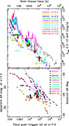 |
Fig. C.1. Comparison of the afterglow light curves of a sample of high-redshift GRBs (color-coded) to our data (cyan stars). Top: Unabsorbed X-ray luminosity (0.3-10 keV), deduced for GRB250314A from the SVOM/MXT, Swift/XRT, and Einstein Probe/FXT data in Table C.1, and obtained through the Swift burst analyser (Evans et al. 2010) for the other high-redshift GRBs. Bottom: Optical light curves. Each rest-frame light curve is shifted to a common z = 7.3 redshift and to the H band. Only detections redwards of the Ly-α break are included. Optical light curves of high-redshift afterglows are taken from Tanvir et al. (2018) and references therein, Rossi et al. (2022), Brivio et al. (2025). |
Results of the spectral analysis of the Swift/XRT and Einstein Probe/FXT X-ray follow-up observations.
In all cases the best fit is obtained by an absorbed power law, with NH fitted values in excess of the Galactic one. Interestingly, we notice that when trying to account for this excess by modelling it as the intrinsic host galaxy hydrogen column density contribution, we obtain values that are in excess of N > 1023 cm−2. Such a large amount of
  has been previously reported for other high-z GRBs, such as GRB 090429B (Cucchiara et al. 2011) and GRB 090423 (Salvaterra et al. 2009), and could be due to an additional contribution of the intergalactic medium (IGM), as pointed out by Starling et al. (2013). We hence examined all available XRT data from the high-redshift sample (11 GRB z > 5.9), applying a model that includes both a local galactic absorber and an intrinsic component from the host galaxy. In all cases, we find an intrinsic column density exceeding 1022 cm−2 (see Fig. C.2), similar to the burst discussed here, supporting the host plus IGM scenario.
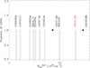 |
Fig. C.2. Distribution of the best-fit values and upper limits for the |

Appendix D: VT data reduction
VT follow-up observations lasted for 3 orbits continuously during the full Moon phase. Although the angular distance to the Moon was 25°, the stray light strength from the Moon in VT images was negligible.
D.1. Quick-look analysis
The on-board data processing pipeline processed the images with four sequences, two performed during the first orbit, and two during the second orbit, aiming to generate the quick look products to have a rapid identification of an optical counterpart. During the processing, the quality of images were checked mainly based on the stability of the platform and background level. The instrument calibrations including bias, dark and LED flat-field correction were then carried out.
Using sub-images centred at the ECLAIRs localisation with a size covering partially the ECLAIRs error-box, the on-board processing pipeline generates source lists for the four sequences and 1-bit images for the first and second sequences (MXT localisation would have been used if it had been available; in this case the sub-images size cover the entire MXT error-box). The source lists contain the sources above the detection threshold, which is configurable on-board with a default value of 2σ (S/N per pixel). The 1-bit images are combined sub-images digitised with 0 or 1 (1-bit) depending if the pixel is below or above the detection threshold. This is adapted to the limited data rate of the VHF network. After being encoded with the Run-Length Encoding method, 1-bit images are near two orders of magnitude smaller than the original images (16 bits). In the case of GRB 250314A, the sub-image transmitted to the ground by the VHF network was generated by stacking six consecutive images and was covering ∼ 55% of the ECLAIRs error-box.
Once the VHF data (source list and 1-bit sub-image) were received, the on-ground real-time data processing pipeline made the astrometric and photometric calibrations. The source lists were cross-checked with known catalogued sources, with a visual check by scientists on duty. The results of this quick-look analysis suggested with high confidence level that there are no uncatalogued sources brighter than 20 mag (Palmerio et al. 2025).
D.2. X-band data analysis: Deep optical upper limits
When X-band data were received later, a more refined analysis was performed, by stacking more calibrated images. Focusing on the precise localisation provided by Swift/XRT (Kennea et al. 2025), and after excluding fake sources caused by detector defects and faint catalogued sources, no optical candidate was detected down to the deep 3 sigma upper limits provided in Table D.1. The corresponding finding chart for the stacked image in VT_R channel (650-1000 nm) is shown in Fig. D.1.
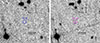 |
Fig. D.1. VT stacked image in VT_B and VT_R bands. The total effective exposure time is 24×50 s and 23×50 s for VT_B and VT_R bands, respectively, at a mid-time of 13.9 min after the burst. The upper represents the north, and the left represents the east. The central red circle denotes the location of GRB 250314A. No signal is detected. |
VT 3σ upper limits for GRB 250314A.
Appendix E: Ground-based optical-NIR follow-up
E.1. Photometry
The data reduction of the VLT/HAWK-I observations reported in Sect. 2 was carried out using the standard ESO pipeline. Near-IR photometric calibration was performed against the VHS catalogue. The small lever arm between J and H does not provide strong constraints on the spectral slope, but formally we find β = 0.19 ± 0.40, where flux density is expressed as a power-law function of frequency, Fν ∝ ν−β. This is relatively blue for a GRB afterglow, suggestive of a low extinction line of sight.
The much steeper slope between the Y and J bands, and deep non-detection in z indicates a sharp spectral break around λ ≈ 1 μm.
E.2. Optical-NIR spectral analysis
The VLT/X-shooter observations, also reported in Sect. 2, consisted of 4 exposures of 1200 s each. These observations were conducted using the ABBA nod-on-slit mode. Each individual VIS spectrum was reduced using the STARE mode reduction, while the NIR arm data was processed using the standard X-shooter NOD mode pipeline (Modigliani et al. 2010). Sky features were subtracted and each flux-calibrated spectrum combined into a final science product (Selsing et al. 2019). All magnitudes are reported in Table E.1.
Optical and NIR ground-based photometry.
To reveal the faint continuum in the X-shooter spectrum shown in Fig. 2 (left), we first masked bad pixels and subtraction residuals of bright sky lines, then binned the VIS (NIR) into 2.5 (1.5) nm wide channels using inverse variance weighting. The extraction was performed using weighting derived from a Gaussian fit to the spatial profile of the trace in the NIR arm. No correction was made for slit losses, although this correction is expected to be small, given the good seeing conditions (∼0.55 arcsec). As discussed in Sect. 2, this analysis revealed a flat continuum with a sharp drop off consistent with the Lyman-α break due to absorption from neutral hydrogen at a redshift of z ≃ 7.3.
Fitting the spectrum (from 0.8 μm to 1.8 μm clipping out regions of bad atmospheric transmission) with a power-law continuum and Lyman-α damping wing, produces a refined redshift estimate of  . Here we assumed negligible dust extinction, adopted a flat prior on the logarithm of the neutral hydrogen column of the host galaxy (i.e. uniform between
  ), and also took the neutral fraction of the intergalactic medium to be XHI = 0.5. The last assumption is reasonable at roughly the mid-point of the re-ionisation era (Planck Collaboration VI 2020), but the results are only weakly dependent on this.
Full corner plots of the parameters from our MCMC fitting are shown in Fig. E.1. The best fitting model is plotted over the spectrum in Fig. 2, and provides an acceptable match to the data with a reduced χν2 = 1.06 for 369 degrees of freedom. We caution that the location of the break close to boundary between the VIS and NIR arms may introduce some extra systematic noise, potentially leading to a small underestimate of the errors on derived parameters.
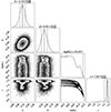 |
Fig. E.1. Corner plots showing the results of our MCMC fitting of a power law plus Ly-α break model to the X-shooter spectrum. Here A denotes overall normalisation, β denotes the spectral slope of the underlying power-law continuum, and NH denotes the host neutral hydrogen column in cm−2 units. |
The assumption of zero dust is justified by the blue spectral slope; which from the X-shooter NIR arm is measured as β = 0.41 ± 0.14, consistent with that found from the photometry. As argued above, this is comparatively blue compared to typical GRB afterglows (e.g. Kann et al. 2010), and together with the absence of detectable deviation from a power-law, indicates low dust extinction in the host. To quantify this further we also performed the model fitting allowing extinction as a free parameter (using the SMC dust law of Pei 1992), and fixing the intrinsic slope to β = 0.5 (consistent with standard fireball models and the X-ray slope estimates reported in Table C.2). This provided a 3σ upper limit for the rest frame visual extinction of AV < 0.09.
In any case, it is important to note that the observed break is considerably sharper than could be produced by any plausible dust feature, and allowing extinction as a free parameter has very little effect on the estimated redshift ( ).
).
The same model fitting prefers low values of host neutral hydrogen column density, but at 3σ allows an upper bound as high as  . The poor S/N means that we are unable to place a meaningful independent constraint on the neutral fraction of the intergalactic medium. However, we note that the S/N in the continuum is still a factor of several times better than the VLT spectra obtained for either GRB 090423 (Tanvir et al. 2009) or GRB 120923A (Tanvir et al. 2018), consistent with the improved redshift precision compared to those events.
Due to the low signal-to-noise, no individual metal absorption features have been confidently identified. EW upper limits could be calculated in different regions of the NIR spectrum (with low atmospheric absorption and good transparency). The S/N is about ∼0.4 (∼0.3) which translates into an EW upper limit rest-frame < 1.5 Å (< 2.6 Å), assuming a 3-σ limit and a nominal X-shooter resolution in the NIR arm of 5600 at 12000 Å. These EW limits are above those typically found in GRB afterglow spectra for the host metal absorption lines detectable in this wavelength range (de Ugarte Postigo et al. 2012).
Appendix F: Radio follow-up
VLA carried out a first set of observations 7 days after Tb, leading to detections at 10 GHz and 15 GHz. The follow-up campaign in radio with ATCA, e-MERLIN and MeerKAT gathered then 10 observations from 9 to 109 days after Tb at several frequencies from 1.3 to 9 GHz.
ATCA data. Following the determination of the spectroscopic redshift, we triggered radio observations with the Australian Telescope Compact Array under programme C3546 (PI Thakur). Observations were obtained in the C (5.5 GHz) and X (9 GHz) bands at one epoch 8.96 days post-burst, for a total of 9.5 hours. The observations in the last two hours were strongly affected by technical issues, resulting in an increased noise level. The datasets were processed in CASA (McMullin et al. 2007) using standard flagging, calibration and imaging procedures. The primary and bandpass calibrator was 1934-638, and the phase calibrator was 1308-098. Flux densities were evaluated at the source peak in the restored images, as this is the best estimate for point-like sources. Root Mean Square (RMS) noise in the final radio maps was computed in an annulus around the source position. The flux error was calculated as the squared sum of the image RMS plus a 5% uncertainty on the flux scale calibration. The source was detected only at 9 GHz at the NIR position. It is not detected at 5.5 GHz, the corresponding 3-sigma upper limit is included in Table F.1.
Radio observations.
e-MERLIN data. We also requested Director’s Discretionary Time observations with the Enhanced Multi-Element Remotely Linked Interferometer Network (e-MERLIN) under programme RR19004 (PI Thakur). They were carried out at C-band (5.1 GHz) and in two epochs, 16.46 and 56.46 days post-burst, including the following antennas: Mk2, Pi, Kn, De, Cm. The phase calibrator was 1332+0509, while 3C286 was adopted for amplitude calibration. The total durations of the two observing runs were ∼36 hours and ∼24 hours, respectively. Data was processed with the e-MERLIN pipeline (Moldon 2021), and imaging was performed with CASA (McMullin et al. 2007) at the central frequency of 5.1 GHz, adopting natural weighting. The RMS was measured in an annulus surrounding the target. The source is not detected at either epoch, the corresponding 3-sigma upper limits are given in Table F.1.
MeerKAT data. We also triggered observations under the MeerKAT programme SCI-20241102-AT-01 (PI Thakur) at L (1.3 GHz) and S2 (2.6 GHz) bands. Observations were conducted at 9.29, 29.2 and 109.10 days post burst, with 30 minutes on-source integration. Phase referencing using 1334-127 as calibrator was applied, while the flux scale calibrator was 1934-738. Data was reduced with the SARAO Science Data Processor (SDP) continuum pipeline. The resulting image has an angular resolution of 8 x 7 arcsec at L band, and 5 x 4 arcsec at S2 band. The average RMS noise level was 10 uJy/beam at L band and 4 uJy/beam at S2 band. The source was not detected at either band in any epoch, the corresponding 3-sigma upper limits are reported in Table F.1.
VLA data. We observed GRB 250314A on 2025 March 21.27 UT at a mean time of 6.7 days after the SVOM trigger with the Karl G. Jansky Very Large Array (VLA) with project VLA/24B-072 (PI: Laskar) using the 3-bit receivers at C, X, and Ku bands (providing 4 GHz, 4 GHz, and 6 GHz bandwidth, respectively). The observations utilised 3C286 as the flux density and bandpass calibrator and J1337-1257 as complex gain calibrator. We reduced the data using the CASA VLA pipeline. Upon imaging the data, we detect a radio counterpart at Ku-band (centre frequency, 15 GHz) and X-band (10 GHz), but not at C-band (6 GHz). We report our point-source fitting photometry results and 3σ upper limits in Table F.1.
Interpretation. Figure F.1 shows the peak flux densities of a sample of GRB radio observations. We highlight the observations of GRBs with z > 6, where GRB 250314A corresponds to the faintest radio detection, although we note the stronger limit for GRB 120923A at z = 7.8. GRB 250314A has a comparable peak luminosity to the also high-z GRB 050904 and GRB 090423 and has a peak luminosity comparable to other lower redshift events. At about 9 days after the burst (1.1 day rest frame) the 9 GHz detection with ATCA, at a flux consistent with the VLA detection, combined with the tight upper limits at lower frequencies (2.6 GHz) by MeerKAT indicate a self-absorbed synchrotron spectrum, typical of a reverse-shock component dominating the radio flux at these early times (≈1 day in the rest frame; e.g. Frail et al. 2000; Laskar et al. 2019). At later times, when the forward shock is expected to dominate, our radio upper limits are 5-10 times lower that the radio emission observed in a burst at a similar redshift (GRB 240218A at z = 6.8, Brivio et al. 2025). This may be attributable to either to a lower energy or a more collimated outflow, with the latter indeed consistent with the steep decay observed in the NIR, that takes place earlier than observed in GRB 240218A.
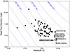 |
Fig. F.1. Observed peak flux densities of the radio emission (∼8 GHz) of long GRBs compared to their redshift. These are adapted from de Ugarte Postigo et al. (2018), using the radio data from Chandra & Frail (2012) updated with high-redshift observations (Tanvir et al. 2012; Rossi et al. 2022; Brivio et al. 2025). The blue lines represent equal luminosity. Note the overlap between the GRB 210905A and GRB 140515A data points. |
Broad-band physical modelling requires an in depth analysis beyond the scope of this paper. We nonetheless adopt a simple synchrotron model to describe the observations. We fit the broad-band spectrum at 0.51 days (12.3 hr) assuming a slow cooling synchrotron spectrum in a constant density environment, with typical slopes of 1/3, −(p − 1)/2 and −p/2, divided by the typical frequencies νm and νc. The spectrum includes the first detection in J band by NOT, while the X-ray flux at 0.51 days is obtained by interpolating the X-ray light curve. We find νc between optical and X-rays, νm below the optical band, and a value of p around 2.5. Letting the model evolve up to the time of the radio detections, we find that the expected forward shock flux is below the radio detection and upper limits, consistent with our inference that the radio afterglow may be dominated by reverse shock emission.
Appendix G: GRB 250314A timeline
We summarise in Fig. H.2 the full observation sequence of GRB 250314A from the ECLAIRs trigger on-board the SVOM satellite to the redshift determination at VLT/X-shooter. We distinguish in this timeline the periods of observations and the times at which the corresponding results became available to the community. As discussed in § 3.2, this highlights the importance of setting up efficient coordination and communication between SVOM and the follow-up collaborations and clearly shows the delays that we should try to shorten.
Appendix H: GRB 250314A energetics and classification
Using the results of the time-integrated joint spectral analysis of ECLAIRs+GRM data presented in Sect. 2 and Appendix B, and adopting a redshift z = 7.3 and the corresponding luminosity distance DL = 74.0 Gpc (using H0 = 67.4 km/s/Mpc, Ωm = 0.315, ΩΛ = 0.685, Planck Collaboration VI 2020), we deduce a burst rest-frame peak energy  keV and an isotropic-equivalent energy
  in the 10 keV–10 MeV energy range (burst rest frame). This value is well below the probable cutoff around ∼4 × 1054 erg in the distribution of the isotropic equivalent energy (Atteia et al. 2025). We compare GRB 250314A to other GRBs in the (1 + z) Ep–Eiso plane (‘Amati relation’; Amati et al. 2002) in Fig. H.1. GRB 250314A is clearly located within the region of long GRBs (type II).
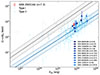 |
Fig. H.1. GRB 250314A in the ’Amati diagram’: The samples of ’short’ (type I, in black) and ’long’ (type II, in blue) GRBs are taken from Lan et al. (2023). The peak energies and isotropic equivalent for the sample of GRBs above z = 6 are taken from Yasuda et al. (2017, GRB130606A, GRB 120521C, GRB 050904A, GRB140515A, GRB080913A, GRB090423A), Rossi et al. (2022, GRB 210905A), Brivio et al. (2025, GRB 240218A), Tanvir et al. (2018, GRB 120923A), Gorbovskoy et al. (2012, GRB 100905A), and Cucchiara et al. (2011, GRB 090429B). All errors are converted to a 68 % confidence level. The properties of GRB250314A (red) are deduced from the results of the joint ECLAIRs+GRM spectral analysis. |
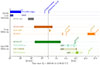 |
Fig. H.2. Observation timeline from the SVOM/ECLAIRs burst detection to redshift determination by VLT/X-Shooter and the announcements in GCN Circulars. The colour-filled blocks show the observation sequence of the different SVOM instruments and follow-up facilities. The shaded blocks for the NOT, GTC, and VLT telescopes represent the local nighttime in the Canary Islands and at Cerro Paranal in Chile. The ’result’ dashed lines for Swift and Einstein Probe indicate the time at which the first X-ray source lists were issued from the XRT and FXT observations, respectively. |
Appendix I: Acknowledgements
The Space-based multi-band Variable Objects Monitor (SVOM) is a joint Chinese French mission led by the Chinese National Space Administration (CNSA), the French Space Agency (CNES), and the Chinese Academy of Sciences (CAS). We gratefully acknowledge the unwavering support of NSSC, IAMCAS, XIOPM, NAOC, IHEP, CNES, CEA, CNRS, University of Leicester, and MPE. We acknowledge the observational data taken at VLT (program 114.27PZ, PIs: Tanvir, Vergani, Malesani), NOT (program P71-506, PIs: Malesani, Fynbo, Xu), GTC (program GTCMULTIPLE4G-25A, PI:Agüí Fernández).
This work also makes use of data obtained with the Einstein Probe, a space mission supported by the Strategic Priority Program on Space Science of the Chinese Academy of Sciences, in collaboration with ESA, MPE and CNES (grant XDA15310000). We acknowledge the use of public data from the Swift data archive. The Australia Telescope Compact Array is part of the Australia Telescope National Facility (https://ror.org/05qajvd42) which is funded by the Australian Government for operation as a National Facility managed by CSIRO. We acknowledge the Gomeroi people as the Traditional Owners of the Observatory site. e-MERLIN is a National Facility operated by the University of Manchester at Jodrell Bank Observatory on behalf of STFC, part of UK Research and Innovation. The MeerKAT telescope is operated by the South African Radio Astronomy Observatory, which is a facility of the National Research Foundation, an agency of the Department of Science and Innovation.
AS acknowledges support by a postdoctoral fellowship from the CNES. SDV and BS acknowledge the support of the French Agence Nationale de la Recherche (ANR), under grant ANR-23-CE31-0011 (project PEGaSUS). LP, ALT GB and GG, acknowledge support by the European Union horizon 2020 programme under the AHEAD2020 project (grant agreement number 871158). LP, ALT and GG also acknowledge support by ASI (Italian Space Agency) through the Contract no. 2019-27-HH.0. NRT acknowledges support from STFC grant ST/W000857/1. The authors are thankful for support from the National Key R&D Program of China (grant Nos. 2024YFA1611704,2024YFA1611700). This work is supported by the Strategic Priority Research Program of the Chinese Academy of Sciences (Grant No.XDB0550401), and by the National Natural Science Foundation of China (grant Nos. 12494575, 12494571, 12494570 and 12133003).
All Tables
Results of the spectral analysis of the Swift/XRT and Einstein Probe/FXT X-ray follow-up observations.
All Figures
|
Fig. 1. Background subtracted light curves for ECLAIRs in the4–100 keV energy range (top panel) and for GRM in the 15–300 keV energy range (bottom panel) using a time bin of 1 s. |
| In the text | |
|
Fig. 2. Left: 2D VIS (top) and NIR (bottom) VLT/X-shooter spectra. The VIS spectrum is cut at 8000 Å, and the vertical dashed black line marks the position corresponding to the Ly-α observer frame wavelength at z ≃ 7.3. Right: 1D re-binned combined spectrum from 9000 to 13 000 Å. The solid red line shows the best fitting afterglow model (Appendix E). Note that the increased noise around the break location is an unfortunate consequence of it being close to the boundary between the VIS and NIR arms. |
| In the text | |
|
Fig. A.1. Location of the burst on the sky in Galactic coordinates (red point). The four alert packets produced by the trigger (inset) have coherent source positions, located well inside the 90 % c.l. error ellipses. |
| In the text | |
|
Fig. A.2. SVOM/ECLAIRs VHF shadow-gram (left) showing the number of counts per detector plane pixel during the time period of the best alert. De-convolved full-sky image (middle) is expressed in units of S/N (σ). A zoom-in on the detected source in the sky image is shown on the right. |
| In the text | |
|
Fig. B.1. Observed T90 duration as a function of the redshift for the current sample of GRBs above z ∼ 6. The observed T90 duration in 4–100 keV of GRB 250314A is shown in red. The observed T90 durations in 15–150 keV of the other bursts in blue are taken from the Swift/BAT catalogue (Lien et al. 2016). The dotted green line corresponds to a duration of 2 s in the burst rest frame. |
| In the text | |
|
Fig. B.2. Best-fit parameters of the ECLAIRs and GRM joint spectral fits using a CPL model in the 5 keV – 5 MeV energy band. Errors are quoted at the 1 σ level. |
| In the text | |
|
Fig. C.1. Comparison of the afterglow light curves of a sample of high-redshift GRBs (color-coded) to our data (cyan stars). Top: Unabsorbed X-ray luminosity (0.3-10 keV), deduced for GRB250314A from the SVOM/MXT, Swift/XRT, and Einstein Probe/FXT data in Table C.1, and obtained through the Swift burst analyser (Evans et al. 2010) for the other high-redshift GRBs. Bottom: Optical light curves. Each rest-frame light curve is shifted to a common z = 7.3 redshift and to the H band. Only detections redwards of the Ly-α break are included. Optical light curves of high-redshift afterglows are taken from Tanvir et al. (2018) and references therein, Rossi et al. (2022), Brivio et al. (2025). |
| In the text | |
|
Fig. C.2. Distribution of the best-fit values and upper limits for the |
| In the text | |
|
Fig. D.1. VT stacked image in VT_B and VT_R bands. The total effective exposure time is 24×50 s and 23×50 s for VT_B and VT_R bands, respectively, at a mid-time of 13.9 min after the burst. The upper represents the north, and the left represents the east. The central red circle denotes the location of GRB 250314A. No signal is detected. |
| In the text | |
|
Fig. E.1. Corner plots showing the results of our MCMC fitting of a power law plus Ly-α break model to the X-shooter spectrum. Here A denotes overall normalisation, β denotes the spectral slope of the underlying power-law continuum, and NH denotes the host neutral hydrogen column in cm−2 units. |
| In the text | |
|
Fig. F.1. Observed peak flux densities of the radio emission (∼8 GHz) of long GRBs compared to their redshift. These are adapted from de Ugarte Postigo et al. (2018), using the radio data from Chandra & Frail (2012) updated with high-redshift observations (Tanvir et al. 2012; Rossi et al. 2022; Brivio et al. 2025). The blue lines represent equal luminosity. Note the overlap between the GRB 210905A and GRB 140515A data points. |
| In the text | |
|
Fig. H.1. GRB 250314A in the ’Amati diagram’: The samples of ’short’ (type I, in black) and ’long’ (type II, in blue) GRBs are taken from Lan et al. (2023). The peak energies and isotropic equivalent for the sample of GRBs above z = 6 are taken from Yasuda et al. (2017, GRB130606A, GRB 120521C, GRB 050904A, GRB140515A, GRB080913A, GRB090423A), Rossi et al. (2022, GRB 210905A), Brivio et al. (2025, GRB 240218A), Tanvir et al. (2018, GRB 120923A), Gorbovskoy et al. (2012, GRB 100905A), and Cucchiara et al. (2011, GRB 090429B). All errors are converted to a 68 % confidence level. The properties of GRB250314A (red) are deduced from the results of the joint ECLAIRs+GRM spectral analysis. |
| In the text | |
|
Fig. H.2. Observation timeline from the SVOM/ECLAIRs burst detection to redshift determination by VLT/X-Shooter and the announcements in GCN Circulars. The colour-filled blocks show the observation sequence of the different SVOM instruments and follow-up facilities. The shaded blocks for the NOT, GTC, and VLT telescopes represent the local nighttime in the Canary Islands and at Cerro Paranal in Chile. The ’result’ dashed lines for Swift and Einstein Probe indicate the time at which the first X-ray source lists were issued from the XRT and FXT observations, respectively. |
| In the text | |
Current usage metrics show cumulative count of Article Views (full-text article views including HTML views, PDF and ePub downloads, according to the available data) and Abstracts Views on Vision4Press platform.
Data correspond to usage on the plateform after 2015. The current usage metrics is available 48-96 hours after online publication and is updated daily on week days.
Initial download of the metrics may take a while.