| Issue |
A&A
Volume 704, December 2025
|
|
|---|---|---|
| Article Number | A72 | |
| Number of page(s) | 18 | |
| Section | Stellar structure and evolution | |
| DOI | https://doi.org/10.1051/0004-6361/202556788 | |
| Published online | 01 December 2025 | |
Old Galactic novae in the eROSITA All-Sky Survey
1
Departament de Física, EEBE, Universitat Politècnica de Catalunya, c/Eduard Maristany 16, 08019 Barcelona, Spain
2
Institut d’Estudis Espacials de Catalunya (IEEC), c/ Esteve Terradas 1, 08060 Castelldefels (Barcelona), Spain
3
Max-Planck-Institut für extraterrestrische Physik (MPE), Gießenbachstraße 1, 85748 Garching, Germany
4
Leibniz-Institut für Astrophysik Potsdam (AIP), An der Sternwarte 16, 14482 Potsdam, Germany
5
Potsdam University, Institute for Physics and Astronomy, Karl-Liebknecht-Straße 24/25, 14476 Potsdam, Germany
⋆ Corresponding author: This email address is being protected from spambots. You need JavaScript enabled to view it.
Received:
8
August
2025
Accepted:
9
September
2025
Abstract
Context. Nova explosions occur on accreting white dwarfs. A thermonuclear runaway in the H-rich accreted envelope causes its ejection without destroying the white dwarf, and an increase in the luminosity by several magnitudes. Accretion is re-established some time after the explosion. The explosion of the nova itself is expected to affect the mass-transfer rate from the secondary and the accretion rate, but these effects have been little explored observationally. Most novae are observed only in outburst, and the properties of the host systems are unknown.
Aims. X-ray observations of novae happen mostly during outburst; only a few have been the target of dedicated X-ray observations years or decades after outburst. However, the X-ray emission long after the outburst provides a powerful diagnostic of the accretion rate and the possible magnetic nature of the white dwarf.
Methods. We explored the first two years of the SRG/eROSITA All-Sky Survey (eRASS) for X-ray sources correlated with Galactic historical novae. We present the first population study of nova hosting systems in X-rays, focusing on the evolution of the accretion rate as a function of time since the last outburst, and look for new candidates for magnetic systems.
Results. In total, 32 X-ray counterparts of novae are found in the western Galactic hemisphere. Combined with 53 nova detections published for the eastern hemisphere, the fraction of X-ray detected novae in quiescence is 18% of the Galactic novae. We have, for the first time, enough statistics to observationally determine the evolution of accretion rate as a function of time since the last nova outburst for a time span of 120 years. The results confirm that magnetic systems remain systematically at higher fluxes and that accretion is enhanced during the first years after the outburst, as theoretically predicted. We also identify new intermediate polar candidates in AT Cnc and RR Cha.
Key words: novae, cataclysmic variables / X-rays: binaries / X-rays: individuals:: AT Cnc / X-rays: individuals:: BD Pav
© The Authors 2025
 Open Access article, published by EDP Sciences, under the terms of the Creative Commons Attribution License (https://creativecommons.org/licenses/by/4.0), which permits unrestricted use, distribution, and reproduction in any medium, provided the original work is properly cited.
This article is published in open access under the Subscribe to Open model. This email address is being protected from spambots. You need JavaScript enabled to view it. to support open access publication.
1. Introduction
Nova outbursts are thermonuclear explosions in the accreted envelope of a white dwarf (WD). Most novae occur in cataclysmic variables (CVs), binary stellar systems with a low-mass donor transferring material to the WD via Roche lobe overflow and forming an accretion disk. In some systems, the WD accretes directly from the dense wind of a red giant companion in a wider binary system. The mechanism of mass accretion (disk or wind) does not affect the final outcome of the WD’s accreted envelope: the H-rich material freshly accumulated under extreme conditions will ignite, triggering a thermonuclear runaway that ultimately leads to the ejection of (most of) the accreted envelope. Novae eject 10−7 − 10−4 M⊙ of material enriched with freshly synthesised elements at velocities of several thousands km s−1 (José & Hernanz 1998; Starrfield et al. 2016).
Nova explosions are relatively frequent events: the estimated Galactic rate is  novae per year (Shafter 2017). However, only about one-fifth of these events are observable, and most of them are lost because of the extinction. In contrast to Type Ia supernovae (SNIa), neither the WD nor the binary system is disrupted during a nova outburst. Novae indeed constitute recurrent phenomena, with expected periodicity of 104 − 105 years in most cases. The most interesting subclass is recurrent novae (RNe), defined by more than one observed outburst, with a periodicity of 1–100 years. Only ten objects belong to this class (Darnley 2021). The higher recurrence frequency points to a larger WD mass, close to the Chandrasekhar limit, and a high accretion rate, making them potential candidates for SNIa progenitors (Selvelli et al. 2003; Kato & Hachisu 2012).
While the general picture is well understood, the details of the processes are full of unknowns. As an example, the initial fireball phase of the explosion predicted by theory for decades was only recently detected for the first time thanks to eROSITA (König et al. 2022). Another point of interest and focus of current debates in the field is the contribution of novae to the lithium present in the Galaxy (after the first detection of Li from Nova Del 2013 by Tajitsu et al. 2015), or the mechanisms powering the very high energy emission (Abdo et al. 2010), probing the high-energy shocks and particle acceleration occurring in the ejecta already predicted some years before (Tatischeff & Hernanz 2007).
The X-ray band is one of the most important diagnostics for novae. In outburst, nova X-rays arise in the form of supersoft emission from direct hydrogen burning on the WD surface, and on a wider X-ray band extending to harder energies from the expanding, shocked ejecta. In addition, the accretion-powered X-ray emission, arising soon or later after the outburst, probes the re-established accretion onto the WD. High-resolution spectroscopy allows us to disentangle the energetics and composition of the atmosphere and the ejecta, while the variability of the X-ray emission often indicates asymmetries in the system (Sala et al. 2008). X-ray emission is also a powerful diagnostic tool for the accretion status of novae after outburst, pointing out the reformation or status of the disk after the explosion (Hernanz & Sala 2002; Ness et al. 2012).
Cataclysmic variables are the host systems of most nova explosions. The formation of the WD, shrinking to a smaller size, induces fast rotation of the final object (by conservation of angular momentum) and, in some cases, the resulting dynamo powers a strong magnetic field. The companion (donor) star fills its own Roche-Lobe and transfers matter from its outer layers to the WD through the inner Lagrangian point, forming an accretion disk around the WD. The matter in the accretion disk gets hot and bright due to the viscosity in the gas, thus radiating energy and losing angular momentum and migrating to the inner radii in the disk until it finally accretes onto the WD surface. Depending on the strength of the magnetic field, the accretion disk might be truncated before the material reaches the WD surface (intermediate polar system, IP) or, if the magnetic field is strong enough, it may completely disrupt the accretion disk (polar). In all magnetic systems, the accretion stream is funnelled onto the WD magnetic poles. The supersonic accreting material becomes subsonic close to the WD surface, creating a shock that ionises the plasma to X-ray emitting temperatures (see Mukai 2017, for a review).
While CVs are relatively faint, and thus their population is best known in the solar neighbourhood (see the volume-complete population study up to 150 pc by Pala et al. 2020), the nova outburst increases the system’s brightness by 7–8 magnitudes. This makes nova events detectable at any distance in the Galaxy and even at extragalactic distances (Shafter 2019). In most cases, however, after the nova outburst is over, the underlying CV remains forgotten or even unreachable. The number of nova progenitors known and characterised is limited (Darnley et al. 2012; Williams et al. 2014, 2016). Accretion is, however, observed to be re-established in several cases soon after the outburst, and this accreting CV can power an X-ray source with luminosities expected in the range 1033 − 1035 erg s−1. The accreting column emits as a shocked thermal plasma with typical temperatures of a few kilo-electronvolts in magnetic novae, while in non-magnetic systems, the equatorial accretion boundary layer powers a fainter and relatively colder X-ray spectrum. In both cases, however, the spectral emission ranges up to several kilo-electronvolts, with interstellar absorption only affecting the softer part of the spectrum but not completely hiding the source. Therefore, X-ray spectra of the host CV provide crucial information for characterising the system, including the magnetic nature of the WD, the accretion rate, the mass of the WD, and the abundances of the accreted material (Mukai 2017). The possibility of nova outbursts occurring on magnetic WDs was questioned in the past (Livio et al. 1988). It was thanks to the detection of coherent modulation in the X-ray data that GK Per (Nova Per 1901) was identified as an IP (Watson et al. 1985). At the same time, Nova Cyg 1975 was recognised as having occurred in a classical polar, V1500 Cyg (Stockman et al. 1988). Since then, a few more novae have been recorded in IP candidates: V1425 Aql (Retter et al. 1998), V2487 Oph (Hernanz & Sala 2002), V4743 Sgr (Kang et al. 2006; Zemko et al. 2016, 2018), V4745 Sgr (Dobrotka et al. 2006), V597 Pup (Warner & Woudt 2009), Nova M31N 2007-12b (Pietsch et al. 2011), V2491 Cyg (Zemko et al. 2015), HZ Pup (Abbott & Shafter 1997; Worpel et al. 2020), V1674 Her (Drake et al. 2021), and V407 Lup (Orio et al. 2024).
During the ROSAT All-Sky Survey (RASS), the positions of 81 old novae were examined, and only 11 of them (14%) were identified as accreting systems (Orio et al. 2001). This study was the last systematic investigation of old novae in the X-ray band. Since the completion of the RASS, more than 200 new nova events have been recorded. More recently, between 2019 and 2022, the eROSITA All-Sky Survey has provided a great opportunity to assess the accretion status of all systems that hosted a nova explosion.
Here, we present the population of old-nova X-ray counterparts detected in the first two years of the eROSITA All-Sky Survey (Predehl et al. 2021). We correlated a catalogue of all nova events recorded in the Galaxy with the western Galactic hemisphere of eRASS:4 DE (German half of data-rights), as well as with the individual surveys eRASS1, eRASS2, eRASS3, and eRASS4. Results from eRASS5 are also included in the present work if the source location was covered by this last partial survey. Considering all historical novae, the evolution of the accretion rate with nova age (years since outburst) can be assessed, thus testing the effect of the nova outburst in the immediate years following the explosion and the long-debated hibernation scenario. In addition, we aim at the identification of new candidates to magnetic systems that have hosted historical nova outbursts. The interest is bidirectional: (a) the first is to understand the effect of the magnetic nature of the host on the nova explosion. With just a few examples of known magnetic CVs hosting novae, and given that each nova explosion has its differential characteristics, the population is too small to identify common patterns, which the magnetic nature of the CV could imprint on the nova explosion. However, we often overlook the magnetic nature of the system for most nova hosts. Therefore, it is of great interest to identify new magnetic nova progenitors and characterise them, including determining the WD mass, magnetic field, and accretion rate. And (b) we aim to understand the effect of the nova explosion on the accretion evolution of the host system. In the classification of CVs as non-magnetic (dwarf novae) and magnetic (IPs and polars), there are some exceptional cases of systems exhibiting dual behaviour, i.e. systems with IP properties that also display dwarf nova outbursts. Hameury & Lasota (2017) reviewed the disk instability model (DIM) to account for the observed dwarf nova outbursts in IPs, concluding that this anomalous behaviour could be related to a historical nova explosion in the system.
In this paper we present the methods used for the data extraction and analysis in Sect. 2. The global population properties and the evolution of X-ray flux over decades are presented in Sect. 3, while Sects. 4 and 5 report the spectral analyses of individual objects with sufficient statistics. Finally, Sections 6 and 7 provide the discussion and summary.
2. Methods
A list of 536 Galactic novae from the 17th century up to 2022 was obtained from the list maintained by Bill Gray1. A first inspection of the list indicated that several Mira stars, low- and high-mass X-ray binaries, transients, and other variable stars were included, probably because they had at some point been incorrectly identified as novae in the literature. We therefore cleaned the list of false novae. Since our main goal is to study the accretion state in the nova-hosting CVs, we also removed symbiotic systems from the sample, as the accretion physics and their X-ray emission are quite different from CVs. We note, however, that the symbiotic nova RR Tel is detected by eROSITA (see Saeedi et al., in prep.). The resulting final list contains 467 novae, with outbursts registered between the 17th century and the year 2022. This final list was correlated using a search radius of 10″ with the catalogues for eRASS1, eRASS2, eRASS3, eRASS4, and eRASS5 (individual eRASS surveys), as well as with the merged eRASS:3 and eRASS:4 catalogues (the stack of the first three and four complete all-sky surveys). All products were produced with the same eSASS version, calibration, and boresight (configuration c030). For the non-detected novae, we computed upper limits using the methods described in Tubín-Arenas et al. (2024).
We checked that the normalised separation between the optical nova position and its X-ray counterparts follows a Rayleigh distribution, as expected, thus confirming the identifications. A few detections of four sources fall at significances larger than 3σ. However, they all correspond to bright sources with small positional error and spectral data that confirm the identification. In particular, RR Pic and CP Pup have large separation σ only in some of the observations (but not all). Moreover, their eROSITA spectra show little variation and are compatible with the spectral results from previous X-ray observations (see Sect. 5). The other two sources with large sigma separation are the novae in outburst (V1710 Sco and YZ Ret), which are affected by pile-up and are not included in further analysis presented in this work.
For historical novae that belong to the eastern Galactic hemisphere with no detection reported in Galiullin & Gilfanov (2021), we determined upper flux limits based on their mirrored position on the western half of the sky. Since the exposure-time map is symmetric in ecliptic coordinates due to the scanning strategy of eROSITA, we mirrored the ecliptic coordinates of the eastern non-detected novae on the sky, and we computed upper limits at the position of these mirrored ecliptic coordinates. We note that by construction, these new mirrored coordinates belong to the western Galactic hemisphere and were observed by eROSITA with the same exposure time as the original coordinates. We confirm that no nearby sources could potentially contaminate the upper limit calculation at the mirrored positions. Thus, in Sect. 3 we include upper limits for sources in the eastern Galactic hemisphere based on the data for the western Galactic hemisphere.
Spectra for sources with more than 50 counts were extracted for the individual eRASS and for the merged eRASS:4. Uncertainties quoted in the text are at 90% confidence, unless otherwise specified. Spectral fitting was done using XSPEC from the HEASOFT package and using cstat statistics. Distances to the correlated novae are listed in Table A.1 with their corresponding reference, in most cases from Gaia DR3 parallaxes (Canbay et al. 2023). The interstellar hydrogen column towards each detected source was obtained from its position and distance using the 3DNH-tool2 developed by Doroshenko (2024); for the non-detected sources, we used the HEASARC NH tool (HI4PI Collaboration 2016).
3. Population properties
In total, 30 eROSITA sources in the western Galactic hemisphere were found to correlate with novae. Table A.1 provides a summary with the list of all the detected novae, their corresponding outburst year, the absorption column, and the distance. The third column of this Table indicates whether the source was detected in the merged eRASS:4 (sm04) or in the merged eRASS:3 (sm03) with no detection in eRASS:4. If it was detected only in an individual eRASS, this is indicated with the label (em0#), where # denotes the eRASS number.
A total of 17 old novae were detected in X-rays for the first time out-of-outburst. Another nine novae had previous X-ray detections out-of-outburst. In addition, four of the novae were detected in outburst or shortly thereafter (YZ Ret 2020, V1706 Sco 2019, V1708 Sco 2020, and V1710 Sco 2021). This represents an increase by a factor of three with respect to the last comparable work with ROSAT (Orio et al. 2001).
Here we present, however, the eRASS:4 results corresponding to the western Galactic hemisphere, and most importantly, with a large fraction in the southern hemisphere. For historical reasons, there is a clear bias towards nova outbursts being detected most frequently in the northern hemisphere; consequently, our half-sky does not represent half of the historical population, but less. Indeed, Galiullin & Gilfanov (2021) reported the historical novae detected by eROSITA in eRASS:3 in the eastern Galactic hemisphere, with Russian data rights, and they reported the detection of 52 historical novae in X-rays. To provide a complete population study of the eROSITA detected novae, we include results from Galiullin & Gilfanov (2021) in several of the population results reported in this section.
Considering the whole sky population, the total number of detected historical novae (not including those detected in outburst) is 83, which represents a fraction of 18% of our full list of old novae. In Fig. 1, the total number of novae, the number of eROSITA detections, and the fraction it represents is shown as a function of age, i.e. years since nova outburst. The uncertainty in the fraction of detected novae was calculated as  , where XRAY is the number of X-ray detected novae and ALL the total number of historical novae for each bin in the histogram.
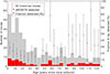 |
Fig. 1. Total number of historical novae (grey bars), novae detected by eROSITA (red bars), and the fraction of eROSITA X-ray detected novae (black bullets, auxiliary right vertical axis) as a function of years since the last nova outburst. eROSITA detections include eRASS:4 DE (this work) as well as detections reported by Galiullin & Gilfanov (2021). |
The location of all eROSITA detections of historical novae is shown in Fig. 2, where the location of the whole sample of historical novae included is also shown. The distribution of all historical novae follows stellar density in the Galaxy, with novae more frequently found in the Galactic plane and towards the Galactic Centre. Inspection of the sky distribution of X-ray detections, however, gives a clear impression of a deficit of X-ray detected novae towards the Galactic centre, most likely due to interstellar absorption. This effect is confirmed in Fig. 3, which shows the distribution of total novae and eROSITA detected novae as functions of Galactic latitude and longitude, along with the fraction of detections.
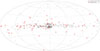 |
Fig. 2. Galactic distribution of all historical novae (grey) and of novae detected in X-rays by eROSITA (red). eROSITA detections include eRASS:4 DE (this work) as well as detections reported by Galiullin & Gilfanov (2021). |
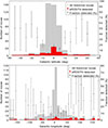 |
Fig. 3. Total number of historical novae (grey bars), novae detected by eROSITA (turquoise bars), and the fraction of eROSITA X-ray detected novae (in black) as a function of Galactic latitude (upper panel) and longitude (lower panel). eROSITA detections include eROSITA_DE eRASS:4 (this work) as well as the detections reported by Galiullin & Gilfanov (2021). |
To further understand the distribution of the eROSITA sample of novae in the Galaxy, we show in Fig. 4 the distribution in age (as years since the last nova outburst), distance, interstellar hydrogen column, and unabsorbed X-ray fluxes. We show both the novae detected in the western Galactic hemisphere in eRASS:4, presented for the first time in this work (see also Table A.1), and the distribution of all the eROSITA detected novae across the whole sky, including those reported for the eastern Galactic hemisphere by Galiullin & Gilfanov (2021). The unabsorbed X-ray fluxes shown in Fig. 4 were determined assuming a 10 keV thermal plasma emission for the novae of the present work. We checked that the precise value of the temperature (in the range 5−15 keV) does not significantly affect the flux within statistical uncertainties. For the novae reported in Galiullin & Gilfanov (2021), which are included in the figures in the present work, only unabsorbed luminosities are reported by the authors. The distances assumed for each nova by the authors are also reported in Galiullin & Gilfanov (2021) and come from different sources, some of which are known to be outdated. Therefore, we corrected the distances to some objects in Galiullin & Gilfanov (2021) to recalculate the luminosity. We first used the luminosity and distance reported by Galiullin & Gilfanov (2021) for each source to determine the unabsorbed flux and then recalculated the unabsorbed luminosities with distances from Bailer-Jones et al. (2021).
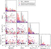 |
Fig. 4. All-sky distributions of all novae detected by eROSITA (red), novae from the western Galactic hemisphere (blue), and upper limits for all non-detected novae in both hemispheres (grey). Distributions of age, distance, interstellar hydrogen column, and X-ray flux (0.2–2.3 keV) are shown. All-sky detected novae and upper limits include eastern Galactic hemisphere results reported in Galiullin & Gilfanov (2021). |
Although the statistical numbers are low, Fig. 4 effectively illustrates the distribution of detected versus non-detected novae. In the distance distribution, it is clear that most detected novae are at distances shorter than 3 kpc, while the non-detected novae with eROSITA peak at distances close to the Galactic Centre, where historical novae cluster, as seen in Fig. 2. Clearly, the absorbing column also plays a role in the detection or non-detection of the objects, with a clear peak of non-detected objects at values of NH ∼ (3 − 5)×1021 cm−2 and most detected novae at NH having values smaller than 2 × 1021 cm−2. Lastly, the upper limits indicated for the non-detected novae in the flux panel show that most novae with fluxes smaller than 6 × 10⁻¹⁴ erg cm−2 s−1 are not detected, although in some cases longer exposure times in that particular position have led to the detection of sources with similar fluxes.
For the novae in the western Galactic hemisphere (eROSITA_DE catalogue), we provide the detailed results for each individual survey as well as for the merged surveys in Table A.2. The count rate and total counts, the uncertainty in the X-ray position and the separation of the X-ray source from the SIMBAD coordinates of the optical nova, hardness ratios, and observation dates for each individual eRASS are reported in Table A.2. In some cases, the source is not detected in one or more individual eRASS, or is detected only in the merged eRASS:4, but not in any of the individual visits. We checked in all cases the upper limits for each individual eRASS with a non-detection of a source that was detected in the merged or other individual eRASS. We find that the upper limits on individual eRASS of sources detected in other eRASS are well compatible with the detected fluxes, and therefore do not indicate intrinsic X-ray variations of the source. Figure 7 shows the light curves of the novae detected in at least four of the individual eRASS.
With the distance and interstellar hydrogen column identified for the sources in Table A.2, we can determine their unabsorbed X-ray luminosity. Since they all consist of CVs years after the nova thermonuclear outburst, we can safely assume that accretion is the only source of X-ray emission and use the unabsorbed X-ray luminosity to estimate the accretion rate. Thus, we can provide for the first time a population study of the accretion rate of novae for the first decades following the outburst, as shown in Fig. 5. Since the cooling flow model (mkcflow in XSPEC) is the model that best represents our available spectral data (see the next section), we obtained a conversion factor from the 0.2−2.3 keV unabsorbed luminosity to mass accretion rate (as part of the normalisation of the mkcflow model) by simulating eROSITA spectra in XSPEC for the range of luminosities of interest. With the conversion factor obtained, we show in Fig. 5 the evolution of the accretion rate in the first 12 decades after a nova outburst. Known magnetic CVs are shown in red.
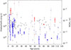 |
Fig. 5. Unabsorbed X-ray luminosity as detected by eROSITA for historical novae located in the western Galactic hemisphere by eROSITA_DE eRASS:4 (big points in red and blue with coloured error bars) as a function of years since the last nova outburst. Known magnetic systems are shown in red. Small points with grey error bars show the novae reported from the eastern Galactic hemisphere by Galiullin & Gilfanov (2021). Upper limits for both hemispheres are shown as grey triangles. |
One interesting characteristic of the host system is the magnetic field of the WD, in particular, whether it is strong enough to disrupt the accretion disk and channel the accretion to the magnetic poles, i.e. whether the host system is a non-magnetic CV, an IP, or a polar. A key characteristic of the magnetic system is the reflection of the X-ray emission from the accretion column on the poles by the WD surface: the heated surface emits as a blackbody, adding an extra soft component to the otherwise pure thermal plasma X-ray spectrum. Our sample has just a few sources with enough statistics for spectral analysis, so the search for such a soft component can be performed only for a few sources (see the next section). However, for the low-statistic sources, a soft excess would in principle make the global X-ray spectrum softer. This could be identified in the hardness ratio, as shown for the global CV population in the eROSITA survey by Schwope et al. (2024).
With the aim of identifying new magnetic candidates, we show the hardness ratio plot for our nova sample in Fig. 6, and list all data in Table A.2. The X-ray hardness ratio is defined as  where H and S are counts in a hard and a soft band, respectively. HR1 corresponds to the ratio of bands S = (0.2 − 0.5) keV and H = (0.5 − 1.0) keV, and HR2 to the bands S = (0.5 − 1.0) keV and H = (1.0 − 2.0) keV. We show the known magnetic systems in red and find that they are not systematically softer in the hardness-ratio plot. As illustrated for the particular case of AT Cnc in the next section, absorption plays a key role, making the position in the hardness ratio plot insensitive to the presence of the soft component.
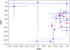 |
Fig. 6. Hardness ratio plot for all eRASS:4 DE historical novae. Known magnetic systems are shown in red. |
4. Spectral results: New bright X-ray counterparts to old novae
4.1. AT Cnc: An intermediate polar masquerading as a dwarf nova?
AT Cnc was discovered as a variable star in 1968 (Romano & Perissinotto 1968) and is traditionally classified as a dwarf nova of the Z Cam type, exhibiting normal outbursts and standstills typical of its class. The long-term light curve available in the AAVSO archives since its discovery shows that standstills of AT Cnc are unusually short (by a few weeks). However, it sometimes reveals abnormally long standstills of about half a year, with visual magnitudes in the range 13−14 (while the full range of variation in its visual magnitude is 12.1−15.4). Nogami et al. (1999) reported time-resolved spectroscopy during a standstill, measuring an orbital period of 0.2011 ± 0.0006 days from the Hα line. They also detected Na I absorption lines in the spectrum. The origin of both Na I and Hα lines was unclear (disk or secondary), although this second option seemed unlikely to Smith et al. (1997) because of the absence of TiO bands.
Shara et al. (2012) discovered a nova shell around AT Cnc, indicating an old nova explosion 330 years ago (Shara et al. 2017), possibly corresponding to the ‘guest star’ reported in the constellation of Cancer by Korean observers in the year 1645 CE. They also determined the distance to AT Cnc to be 460 pc, consistent with results from Gaia DR3 (455 ± 7 pc, Canbay et al. 2023).
Kozhevnikov (2004) reported the detection of superhumps for the first time in a Z Cam system, indicating an asymmetric accretion disc. More recently, the first suggestion of the possible magnetic nature of AT Cnc appeared in the coherent brightness modulations reported by Bruch et al. (2019). In addition to the orbital period of 0.2 days (290 min), they find a new modulation of 25.7 minutes, most probably corresponding to the WD spin. As the authors suggest, all this points to the possibility of an IP scenario.
eROSITA provides the first registered X-ray detection of the system. Individual eRASS spectra are shown in Fig. 8 and lack the S/N for spectral analysis. However, it is evident that the count rate is much lower in the first eRASS than in the following three, with just a marginal detection in eRASS1. The spectral energy distribution remains similar for the three following spectra obtained 0.5, 1, and 1.5 years afterwards. We considered the merged eRASS:4 spectra for spectral analysis. The total count rate from eRASS:4 extracted from the catalogue is 0.254 ± 0.031 cts s−1. For spectral fitting, we used the merged eRASS:4 manually extracted spectrum binned to contain at least 5 counts per bin, which, after background subtraction and loading it in XSPEC, has a net count rate of 0.09 ± 0.02 cts/s and a total exposure time of 571 s.
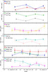 |
Fig. 7. Variability in count rate for novae detected in four or five individual eRASS. |
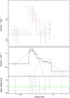 |
Fig. 8. Upper panel: AT Cnc spectra for the merged eRASS:4 (black) and for the individual eRASS1 (red), eRASS2 (blue), eRASS3 (green), and eRASS4 (magenta). Lower panel: merged spectrum for eRASS:4 with the best-fit model. Individual components of the model (blackbody at low energies and mkcflow at higher energies) are shown in dashed lines. |
At first glance, the eRASS:4 spectrum of AT Cnc does not seem to correspond to a single component model (see Fig. 8). The detected rate is maximum at 0.8 keV, and the counts below 0.7 keV are negligible. Taking the results with caution due to the low statistics, the observed spectrum was well reproduced by a soft blackbody component plus a bremsstrahlung, or by a more realistic isobaric cooling flow thermal plasma (mkcflow model), with a low temperature of 500 eV and maximum temperature of 3 keV, but with unconstrained uncertainties. For the other parameters, the uncertainties were determined with the steppar function. Contour plots for the parameters of the black body and the plasma model were determined separately (see Fig. B.1), freezing the parameters of the other model component to the best-fit values. The accretion rate is 5(±3)×10−11 M⊙ yr−1. The soft excess is well fit with a blackbody with kT = 50 ± 10 eV and a lower limit for the bolometric luminosity of 1034 erg s−1. The 0.2−2.3 keV flux with this best fit model to the merged eRASS:4 spectrum is 3.0(±0.5)×10−13 erg cm−2 s−1, corresponding to a total 0.2−2.3 keV luminosity of 7(±1)×1030 erg s−1. We used the upper limit ESA server HILIGT3 to check that the upper limits for the 0.2−2.3 keV flux from the ROSAT All-Sky Survey (< 8 × 10⁻¹³ erg cm−2 s−1) and the XMM-Newton Slew Catalogue (< 4 × 10⁻¹³ erg cm−2 s−1) are compatible with the flux detected by eROSITA.
The position of AT Cnc in the hardness ratio is surprisingly hard for a source with a soft component (HR12 ∼ 0.8, see Table A.2). The reason is that the count rate below 0.7 keV is negligible, suggesting a source of intrinsic absorption. A spectral fit including the lowest energy spectral channels yields an absorbing column of 2(±1)×1022 cm−2. The average interstellar hydrogen column in the direction of AT Cnc is 3.8 × 1020 cm−2 from the H14PI maps (HI4PI Collaboration 2016). Since AT Cnc is at a larger distance to the Sun than the sources included in the H14PI maps in the direction of interest, we checked the reddening from the STILISM maps, which indicate E(B − V) = 0.3 ± 0.1 (Lallement et al. 2014; Capitanio et al. 2017). This corresponds to a hydrogen column of 1.6(±0.1)×1020 cm−2 (using the most widespread E(B − V) relation from Savage et al. 1977 and Bohlin et al. 1978) or 2.3(±0.2)×1020 cm−2 with a more recent determination for the NH/E(B − V) relation (Liszt 2014). So, a local or intrinsic source of absorption seems present. Shara et al. (2012) determined a total mass in the nova shell of 5 × 10⁻⁵ M⊙ and a shell radius of 0.2 pc. Assuming an homogeneous distribution of the ejected mass and pure atomic hydrogen, the column density in the line of sight due to the shell would be only 1017 cm−2. However, the shell is clearly not homogeneous, and the images show that the matter is in blobs of circa 1″ in diameter (Shara et al. 2017).
4.2. BD Pav
BD Pav is a dwarf nova of the U Gem type located at 329 ± 2 pc, which underwent a nova eruption in 1934. Barwig & Schoembs (1983) determined the orbital period to be 4.3 hours, with an exceptionally bright secondary. The light curves in quiescence exhibited sharp eclipses, suggesting a relatively high inclination system. Sion et al. (2008) attempted to determine the WD mass from HST STIS spectra. They fit the data with a 1.2 M⊙ WD with an effective temperature of 27 000 K and an inclination of 75° for the optically thick disk. However, the fit was not good, and the results are to be taken with care. The interstellar hydrogen column in the direction of BD Pav is 6 × 1020 cm−2 (HI4PI Collaboration 2016).
Individual eRASS have a very low S/N (see Fig. 9), so we worked with the merged eRASS:4 results. The total count rate from eRASS:4 extracted from the catalogue is 0.423 ± 0.034 cts s−1. For spectral fitting, we used the manually extracted eRASS:4 spectra, binned to contain at least 5 counts per bin (Fig. 9). The fitted spectral data have a net count rate of 0.13 ± 0.02 cts s−1, with a total exposure time of 811 s. A cooling flow mkcflow model can reproduce the spectrum with a temperature higher than 40 keV (1σ lower limit and upper limit unconstrained; see Fig. B.2), an accretion rate of 5( M⊙ yr−1, and an absorbing hydrogen column density of
  cm−2. A simple absorbed bremsstrahlung provides a similar fit but with unconstrained temperature. The 0.2−2.3 keV flux with the best-fit mkcflow model is 5(±1)×10−13 erg cm−2 s−1, corresponding to a total 0.2−2.3 keV luminosity of 6.5(±2.0)×1030 erg s−1. The flux is compatible with the upper limit from the XMM-Newton Slew catalogue. There are no published results for the X-ray source, and the only previous X-ray detection found in the archives is that of the ROSAT All-Sky Survey from August 1990 with a detection of the source at a count rate of 0.079 ± 0.030 cts s−1, corresponding to a flux of 7.5(±3.2)×10−13 erg cm−2 s−1 (0.2−2.3 keV), likewise compatible with the flux determined presently by eROSITA4.
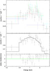 |
Fig. 9. Upper panel: BD Pav spectra for the merged eRASS:4 (black) and for the individual eRASS1 (red), eRASS2 (blue), eRASS3 (green), and eRASS4 (magenta). Lower panel: merged spectrum for eRASS:4 with the best-fit model. |
5. Nova hosts CVs previously known in X-rays: Spectral analysis
5.1. CP Pup
CP Pup is a well-known CV, that experienced a nova outburst in 1942. Orio et al. (2009) obtained XMM-Newton/RGS grating spectra, and their results suggested a high mass and magnetic WD. The XMM-Newton spectra obtained in 2005 were well fit with an isobaric cooling model, mkcflow, with a maximum temperature of 80 keV and an absorbing hydrogen column of 2 × 1021 cm−2, with a flux in the RGS (0.33−2.5 keV) energy range of 2.3(±0.2)×10−12 erg cm−2 s−1. The normalisation constant of the cooling flow model indicated an upper limit for the accretion rate of 8 × 10⁻¹¹ M⊙ yr−1 for a distance of 850 pc – the minimum distance estimation at the time. Mason et al. (2013) based on Chandra/HETG refined the accretion rate to 3.3 × 10⁻¹⁰ M⊙ yr−1 with a maximum temperature of the cooling model at 40(±20) keV and found that the X-ray spectral characteristics were consistent with those of known IPs.
The total count rate from eRASS:4 extracted from the catalogue is 0.89 ± 0.04 cts s−1. For spectral fitting, we used the manually extracted eRASS:4 spectra, binned to contain at least 5 counts per bin (Fig. 10). A cooling flow mkcflow model can reproduce the spectrum with a high temperature of 15( keV and an accretion rate of 5(
 M⊙ yr−1, with NH = 3.0(±1.5)×1021 cm−2. The residuals show possible absorption around 0.65 keV (possibly O VIII). The 0.2−2.3 keV flux with the best-fit mkcflow model is 9(±5)×10−13 erg cm−2 s−1. This flux corresponds to a total 0.2−2.3 keV luminosity of 6(±3)×1031 erg s−1 (at 767 pc as determined from Gaia DR3, Canbay et al. 2023).
5.2. HZ Pup
Evidence of the magnetic nature of HZ Pup (with a 5.11 h orbital period) comes from the identification of a possible spin period (20 minutes, Abbott & Shafter 1997) also detected in the XMM-Newton light curve by Worpel et al. (2020). The same authors fit the faint-phase spectra with a single temperature APEC (15 keV) and add a second APEC model for the bright phase (64 keV). They also added two Gaussian emission lines at 0.5 keV, to account for the soft excess, and at 6.4 keV for the fluorescence Fe line. Table 4 of Worpel et al. (2020) indicates that the X-ray flux for each of the two APEC components used to fit the XMM-Newton spectra is 6 × 10⁻¹² erg cm−2 s−1. The distance to HZ Pup is 2.7(±0.5) kpc from Gaia DR3 (Canbay et al. 2023).
The total count rate from eRASS:4 extracted from the catalogue is 0.227 ± 0.024 cts s−1. For spectral fitting, we used the merged eRASS:4 manually extracted spectra, binned to contain at least 5 counts per bin (Fig. 11). A single cooling flow mkcflow model fails to reproduce the spectrum, which shows clear soft excess. Even allowing for an absorbing hydrogen column orders of magnitude lower than that expected from the interstellar medium (ISM), the plasma model is too flat to reproduce the soft excess. Thus, we added a blackbody model to fit the soft excess. The isobaric cooling flow has a low temperature of 0.1−0.2 keV (free fits were kept around this value even without blackbody components and frozen parameters), while the maximum temperature pegs at a maximum of 80 keV (both without and with the blackbody components present). The accretion rate for the best-fit model is 6.7 × 10⁻¹¹ M⊙ yr−1. The blackbody accounts for the soft excess with a temperature of 50 eV and a normalisation of 4 × 10⁻⁴, which corresponds to 3 × 1034 erg s−1. The X-ray flux 0.2−2.3 keV is 2 × 10⁻¹³ erg cm−2 s−1 (corresponding X-ray luminosity at 2.7 kpc is 2 × 1032 erg s−1).
5.3. RR Pic
RR Pic is classified in the Ritter & Kolb catalogue as an SW Sex star; Orio et al. (2001) considered it to be the only suspected magnetic CV in the old nova ROSAT sample. However, the most recent Chandra observation (Pekön & Balman 2008) found no evidence of a magnetic nature, with the ACIS-S spectra fit using a vmcflow model, with some overabundance of C and O and a maximum temperature of around 2 keV. The distance to RR Pic is now known to be 492(±5) pc from Gaia DR3 (Canbay et al. 2023).
The total count rate from eRASS:4 extracted from the catalogue is 0.280 ± 0.010 cts s−1. For spectral fitting, we used the merged eRASS:4 manually extracted spectra, binned to contain at least 5 counts per bin (Fig. 12). The net rate of the spectrum used to fit was 0.073 ± 0.004 cts s−1, with a total exposure time of 5904 s (448 spectral counts). A cooling flow mkcflow model reproduced the spectrum, leaving some excess above 2 keV (as found by Pekön & Balman 2008 in Chandra spectra). The isobaric cooling flow model that best reproduces the data has a low temperature of 80(±20) eV and a maximum temperature of 3.5 keV, with an accretion rate of 14
 M⊙ yr−1. The X-ray flux of 0.2−2.3 keV is 2.5 × 10⁻¹³ erg cm−2 s−1 (corresponding X-ray luminosity at the distance of RR Pic is 7 × 1030 erg s−1).
5.4. A not-so-old nova, now in quiescence: V407 Lup 2016
V407 Lup (Nova Lup 2016) is thought to have occurred on an IP. Aydi et al. (2018) studied the X-ray SSS emission and found evidence of resumed accretion. They found two periodicities in UV and X-rays at 3.57 h and 565 s, interpreted as the orbital period and the spin of the WD in an IP, which was confirmed with XMM-Newton observations obtained in quiescence in 2020 (Orio et al. 2024). Aydi et al. (2018) also report a complex X-ray spectrum, including a hard component, which could be fit by a flat power law or a relatively high-temperature thermal component.
The eRASS:4 spectrum of the quiescent nova is well fit with a thermal plasma. A single high-temperature Mekal (80 keV) fits reasonably well, similar to a mkcflow model with a low temperature of 100 eV, a maximum temperature pegged at 80 keV, and an accretion rate of 3 × 10⁻¹¹ M⊙ yr−1 (for a 3 kpc distance). With large uncertainty in the distance (Aydi et al. 2018), the statistical uncertainties are not significant. Still, the spectral parameters are consistent with an accreting, isobaric shock flow on a WD. The X-ray flux of 0.2−2.3 keV is 1.2 × 10⁻¹³ erg cm−2 s−1 (corresponding to an X-ray luminosity of 1032 erg s−1).
Best-fit spectral parameters of novae with more than 50 cts s−1 in the merged spectra.
6. Discussion
The evolution of the accretion rate over the first 12 decades after a nova outburst, shown in Fig. 5, clearly indicates a lack of bright sources following the first two decades. The right vertical axis shows the accretion rate corresponding to the observed unabsorbed flux, determined as explained in Sect. 3. Known magnetic CVs are shown in red and clearly have systematic higher X-ray luminosities than non-magnetic systems. While our procedure may have introduced some systematics in the values of the accretion rates obtained, since the conversion factor used was constant for all cases, the evolution as a function of age is not affected by the particular value of the conversion from X-ray luminosity to accretion rate. Therefore, the result of the accretion rate evolution after the nova outburst is robust: there is a clear excess of high-accretion rate systems shortly after the nova outburst, which decreases over the first two decades. After that initial decrease, the accretion rates seem to remain at a similar level in the first century after the outburst. A second view of the same effect, free of any assumptions, is found simply in the fraction of the novae detected in X-rays as a function of time following outburst, in Fig. 1.
One aspect of concern to be considered when assessing the accretion-powered X-ray emission of faint CVs is the possible contribution from the corona of the donor star to the total X-ray luminosity. Schmitt & Liefke (2004) showed from nearby stars in the ROSAT All-Sky Survey that the X-ray luminosity of F, G, K, and M stars very rarely reaches values as large as 1029 erg s−1, with most stars emitting at 1027 − 1028 erg s−1. This is well below the faintest sources of our sample, and thus we can assume that the X-ray luminosities observed are accretion-powered.
The evolution suggested by Fig. 5 agrees with the predicted behaviour of accretion in post-outburst nova systems as modelled by Hillman et al. (2020). The enhanced accretion rate shortly after the nova outburst is explained by the irradiation of the secondary by the hot WD during and short after the nova eruption. This causes the expansion of the secondary, enhancing Roche Lobe overflow and the mass transfer, which ultimately causes an increased accretion rate onto the WD and therefore increased accretion-powered X-ray luminosities. The accretion rate is then predicted to decrease by Hillman et al. (2020) over a few hundred to thousands of years, as the effect of the WD irradiation diminishes. We can provide here the first X-ray observational test for this predicted behaviour. From Fig. 5, we can confirm the initial decay of the accretion rate. This decay, however, seems predominant only for the first 30 years. Our observed X-ray luminosities of quiescent novae seem to stop decreasing after that, indicating that either the WD cooling is faster, or the effect of the irradiated WD on the secondary may be shorter than predicted.
For spectral properties, we limit our studies to the western Galactic hemisphere. A point of interest is to identify new candidates to magnetic systems, and for that we plot the HR1-HR2 hardness ratio diagram in Fig. 6. The systematic study of CVs observed by eROSITA presented by Schwope et al. (2024) shows the distribution of non-magnetic, IP, and polar CVs in the HR1-HR2 hardness plot. It is clear that non-magnetic systems cluster at a higher value of HR1, and only polars and some IPs appear at lower values of HR1. But it is also clear that many of the magnetic systems show HR1-HR2 positions in the region of the non-magnetic systems.
From our HR1-HR2 plot (Fig. 6) we immediately find that most known magnetic systems do not cluster in a particular region of the hardness ratio plot. From the cases where we do have spectra, as in the case of AT Cnc, it seems clearly related to the role of absorption. To further explore the role of absorption in the position of magnetic systems in the HR1-HR2 plot, we simulated the tracks on that plot for a set of spectral models in Fig. 14. We plot the position of simulated eROSITA spectra in the HR1-HR2 diagram in Fig. 14 for a series of models including only thermal plasma components, or adding a soft, blackbody component (indicative of the accretion on the magnetic poles). For each set of models, we simulate the HR1-HR2 tracks for increasing absorption column. It is clear that even with the presence of a soft component, absorption can place the source in the same region of the HR1-HR2 plot as non-magnetic systems.
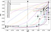 |
Fig. 14. Hardness ratio plot with our detected novae and simulated paths for spectral models with variable absorption hydrogen column (increasing between 1 × 10²⁰ and 2 × 1022 cm−2 from left to right). Pure thermal plasma models (mekal) are shown in dashed lines, with kT increasing from 1 keV (blue, dashed line) to 35 keV. All models with kT above 5 keV collapse on the same path on the plot (red dashed line). Dotted lines show models with an extra soft, blackbody component with effective temperatures from 20 eV (purple) to 90 eV (green). The simulations with a soft component also include a thermal plasma with kT = 15 keV and a normalisation of a factor 10 fainter than the blackbody. Detected historical novae in the eRASS:4 are shown as big dots for new detections, stars for known IPs, and triangles for all other cases. |
7. Summary
We presented a large-scale X-ray population analysis of historical novae observed during the first two years of the eROSITA All-Sky Survey (eRASS:4), focusing on novae in the western Galactic hemisphere. We cross-matched 467 cleaned nova candidates with eROSITA source catalogues and identified 30 old novae in X-rays, 17 of which were detected in X-rays in quiescence for the first time. When combined with previous detections from the eastern Galactic hemisphere reported by Galiullin & Gilfanov (2021), this yields an 18% X-ray detection rate for historical novae in quiescence. The detection of novae from the 20th and 21st centuries reveals a clear trend: accretion rates are higher in the first 20–30 years post-outburst and then stabilise over the following century. A hardness-ratio analysis was attempted to assess the magnetic nature of the WDs, although absorption often obscures soft X-ray components. Some sources are bright enough for spectral analysis, and among them, AT Cnc was identified as a likely IP based on the clear soft excess of its X-ray spectrum.
For the ROSAT flux calculation, we first fit a power-law to the eRASS:4 spectrum to find the best-fit absorption column and slope and checked that the total flux for the eROSITA merged spectrum was the same as for the best-fit model. We then used this power-law parameter to convert the ROSAT count rate to flux.
Acknowledgments
This work is based on data from eROSITA, the soft X-ray instrument aboard SRG, a joint Russian-German science mission supported by the Russian Space Agency (Roskosmos), in the interests of the Russian Academy of Sciences represented by its Space Research Institute (IKI), and the Deutsches Zentrum für Luft- und Raumfahrt (DLR). The SRG spacecraft was built by Lavochkin Association (NPOL) and its subcontractors, and is operated by NPOL with support from the Max Planck Institute for Extraterrestrial Physics (MPE). The development and construction of the eROSITA X-ray instrument was led by MPE, with contributions from the Dr. Karl Remeis Observatory Bamberg & ECAP (FAU Erlangen-Nürnberg), the University of Hamburg Observatory, the Leibniz Institute for Astrophysics Potsdam (AIP), and the Institute for Astronomy and Astrophysics of the University of Tübingen, with the support of DLR and the Max Planck Society. The Argelander Institute for Astronomy of the University of Bonn and the Ludwig Maximilians Universität Munich also participated in the science preparation for eROSITA. The eROSITA data shown here were processed using the eSASS/NRTA software system developed by the German eROSITA consortium. GS acknowledges support by the Spanish MINECO grant PID2023-148661NB-I00, by the E.U. FEDER funds, and by the AGAUR/Generalitat de Catalunya grant SGR-386/2021. GS acknowledges support from the Max-Planck-Institut für extraterrestrische Physik for her summer visits in 2023, 2024, and 2025.
References
- Abbott, T. M. C., & Shafter, A. W. 1997, in IAU Colloq. 163: Accretion Phenomena and Related Outflows, eds. D. T. Wickramasinghe, G. V. Bicknell, & L. Ferrario, ASP Conf. Ser., 121, 679 [Google Scholar]
- Abdo, A. A., Ackermann, M., Ajello, M., et al. 2010, Science, 329, 817 [NASA ADS] [CrossRef] [Google Scholar]
- Aydi, E., Orio, M., Beardmore, A. P., et al. 2018, MNRAS, 480, 572 [Google Scholar]
- Bailer-Jones, C. A. L., Rybizki, J., Fouesneau, M., Demleitner, M., & Andrae, R. 2021, AJ, 161, 147 [Google Scholar]
- Barwig, H., & Schoembs, R. 1983, A&A, 124, 287 [Google Scholar]
- Baumgardt, H., & Vasiliev, E. 2021, MNRAS, 505, 5957 [NASA ADS] [CrossRef] [Google Scholar]
- Bohlin, R. C., Savage, B. D., & Drake, J. F. 1978, ApJ, 224, 132 [Google Scholar]
- Bruch, A., Boardman, J., Cook, L. M., et al. 2019, New Astron., 67, 22 [Google Scholar]
- Canbay, R., Bilir, S., Özdönmez, A., & Ak, T. 2023, AJ, 165, 163 [NASA ADS] [CrossRef] [Google Scholar]
- Capitanio, L., Lallement, R., Vergely, J. L., Elyajouri, M., & Monreal-Ibero, A. 2017, A&A, 606, A65 [NASA ADS] [CrossRef] [EDP Sciences] [Google Scholar]
- Darnley, M. J. 2021, The Golden Age of Cataclysmic Variables and Related Objects V, 2–7, 44 [Google Scholar]
- Darnley, M. J., Ribeiro, V. A. R. M., Bode, M. F., Hounsell, R. A., & Williams, R. P. 2012, ApJ, 746, 61 [NASA ADS] [CrossRef] [Google Scholar]
- Dobrotka, A., Retter, A., & Liu, A. 2006, MNRAS, 371, 459 [Google Scholar]
- Doroshenko, V. 2024, A&A, submitted [arXiv:2403.03127] [Google Scholar]
- Drake, J. J., Ness, J.-U., Page, K. L., et al. 2021, ApJ, 922, L42 [Google Scholar]
- Galiullin, I. I., & Gilfanov, M. R. 2021, Astron. Lett., 47, 587 [CrossRef] [Google Scholar]
- Hameury, J. M., & Lasota, J. P. 2017, A&A, 602, A102 [Google Scholar]
- Hernanz, M., & Sala, G. 2002, Science, 298, 393 [Google Scholar]
- HI4PI Collaboration 2016, A&A, 594, A116 [NASA ADS] [CrossRef] [EDP Sciences] [Google Scholar]
- Hillman, Y., Shara, M. M., Prialnik, D., & Kovetz, A. 2020, Nat. Astron., 4, 886 [Google Scholar]
- Howell, S. B., Reyes, A. L., Ashley, R., Harrop-Allin, M. K., & Warner, B. 1996, MNRAS, 282, 623 [Google Scholar]
- José, J., & Hernanz, M. 1998, ApJ, 494, 680 [Google Scholar]
- Kang, T. W., Retter, A., Liu, A., & Richards, M. 2006, AJ, 132, 608 [Google Scholar]
- Kato, M., & Hachisu, I. 2012, Bull. Astron. Soc. India, 40, 393 [NASA ADS] [Google Scholar]
- König, O., Wilms, J., Arcodia, R., et al. 2022, Nature, 605, 248 [CrossRef] [Google Scholar]
- Kozhevnikov, V. P. 2004, A&A, 419, 1035 [NASA ADS] [CrossRef] [EDP Sciences] [Google Scholar]
- Lallement, R., Vergely, J. L., Valette, B., et al. 2014, A&A, 561, A91 [NASA ADS] [CrossRef] [EDP Sciences] [Google Scholar]
- Liszt, H. 2014, ApJ, 780, 10 [Google Scholar]
- Livio, M., Shankar, A., & Truran, J. W. 1988, ApJ, 330, 264 [NASA ADS] [CrossRef] [Google Scholar]
- Mason, E., Orio, M., Mukai, K., et al. 2013, MNRAS, 436, 212 [NASA ADS] [CrossRef] [Google Scholar]
- Mason, E., Shore, S. N., Drake, J., et al. 2021, A&A, 649, A28 [NASA ADS] [CrossRef] [EDP Sciences] [Google Scholar]
- Merloni, A., Lamer, G., Liu, T., et al. 2024, A&A, 682, A34 [NASA ADS] [CrossRef] [EDP Sciences] [Google Scholar]
- Mróz, P., Udalski, A., Pietrukowicz, P., et al. 2016, Nature, 537, 649 [CrossRef] [Google Scholar]
- Mukai, K. 2017, PASP, 129, 062001P [NASA ADS] [CrossRef] [Google Scholar]
- Ness, J. U., Schaefer, B. E., Dobrotka, A., et al. 2012, ApJ, 745, 43 [NASA ADS] [CrossRef] [Google Scholar]
- Nogami, D., Masuda, S., Kato, T., & Hirata, R. 1999, PASJ, 51, 115 [Google Scholar]
- Orio, M., Covington, J., & Ögelman, H. 2001, A&A, 373, 542 [NASA ADS] [CrossRef] [EDP Sciences] [Google Scholar]
- Orio, M., Mukai, K., Bianchini, A., de Martino, D., & Howell, S. 2009, ApJ, 690, 1753 [Google Scholar]
- Orio, M., Melicherčík, M., Ciroi, S., et al. 2024, MNRAS, 533, 1541 [Google Scholar]
- Pala, A. F., Gänsicke, B. T., Breedt, E., et al. 2020, MNRAS, 494, 3799 [Google Scholar]
- Pietsch, W., Henze, M., Haberl, F., et al. 2011, A&A, 531, A22 [NASA ADS] [CrossRef] [EDP Sciences] [Google Scholar]
- Pekön, Y., & Balman, Ş. 2008, MNRAS, 388, 921 [Google Scholar]
- Predehl, P., Andritschke, R., Arefiev, V., et al. 2021, A&A, 647, A1 [EDP Sciences] [Google Scholar]
- Retter, A., Leibowitz, E. M., & Kovo-Kariti, O. 1998, MNRAS, 293, 145 [Google Scholar]
- Romano, G., & Perissinotto, M. 1968, Mem. Soc. Astron. It., 39, 429 [Google Scholar]
- Sala, G., Hernanz, M., Ferri, C., & Greiner, J. 2008, ApJ, 675, L93 [Google Scholar]
- Savage, B. D., Bohlin, R. C., Drake, J. F., & Budich, W. 1977, ApJ, 216, 291 [NASA ADS] [CrossRef] [Google Scholar]
- Schmitt, J. H. M. M., & Liefke, C. 2004, A&A, 417, 651 [NASA ADS] [CrossRef] [EDP Sciences] [Google Scholar]
- Schwope, A. D., Knauff, K., Kurpas, J., et al. 2024, A&A, 690, A243 [NASA ADS] [CrossRef] [EDP Sciences] [Google Scholar]
- Selvelli, P., Gilmozzi, R., & Cassatella, A. 2003, Mem. Soc. Astron. Ital. Suppl., 3, 129 [Google Scholar]
- Shafter, A. W. 2017, ApJ, 834, 196 [CrossRef] [Google Scholar]
- Shafter, A. W. 2019, Extragalactic Novae; A Historical Perspective (IOP Publishing Ltd) [Google Scholar]
- Shara, M. M., Mizusawa, T., Wehinger, P., et al. 2012, ApJ, 758, 121 [Google Scholar]
- Shara, M. M., Drissen, L., Martin, T., Alarie, A., & Stephenson, F. R. 2017, MNRAS, 465, 739 [NASA ADS] [CrossRef] [Google Scholar]
- Sion, E. M., Gänsicke, B. T., Long, K. S., et al. 2008, ApJ, 681, 543 [Google Scholar]
- Smith, R. C., Sarna, M. J., Catalan, M. S., & Jones, D. H. P. 1997, MNRAS, 287, 271 [Google Scholar]
- Starrfield, S., Iliadis, C., & Hix, W. R. 2016, PASP, 128, 051001 [Google Scholar]
- Stockman, H. S., Schmidt, G. D., & Lamb, D. Q. 1988, ApJ, 332, 282 [Google Scholar]
- Szkody, P., Gänsicke, B. T., Sion, E. M., & Howell, S. B. 2002, ApJ, 574, 950 [Google Scholar]
- Tajitsu, A., Sadakane, K., Naito, H., Arai, A., & Aoki, W. 2015, Nature, 518, 381 [NASA ADS] [CrossRef] [Google Scholar]
- Tatischeff, V., & Hernanz, M. 2007, ApJ, 663, L101 [Google Scholar]
- Tubín-Arenas, D., Krumpe, M., Lamer, G., et al. 2024, A&A, 682, A35 [NASA ADS] [CrossRef] [EDP Sciences] [Google Scholar]
- Warner, B., & Woudt, P. A. 2009, MNRAS, 397, 979 [Google Scholar]
- Watson, M. G., King, A. R., & Osborne, J. 1985, MNRAS, 212, 917 [NASA ADS] [CrossRef] [Google Scholar]
- Whitelock, P. A. 1988, in IAU Colloq. 103: The Symbiotic Phenomenon, eds. J. Mikolajewska, M. Friedjung, S. J. Kenyon, & R. Viotti, Astrophysics and Space Science Library, 145, 47 [Google Scholar]
- Williams, S. C., Darnley, M. J., Bode, M. F., Keen, A., & Shafter, A. W. 2014, ApJS, 213, 10 [Google Scholar]
- Williams, S. C., Darnley, M. J., Bode, M. F., & Shafter, A. W. 2016, ApJ, 817, 143 [NASA ADS] [CrossRef] [Google Scholar]
- Worpel, H., Schwope, A. D., Traulsen, I., Mukai, K., & Ok, S. 2020, A&A, 639, A17 [NASA ADS] [CrossRef] [EDP Sciences] [Google Scholar]
- Zemko, P., Mukai, K., & Orio, M. 2015, ApJ, 807, 61 [Google Scholar]
- Zemko, P., Orio, M., Mukai, K., et al. 2016, MNRAS, 460, 2744 [Google Scholar]
- Zemko, P., Ciroi, S., Orio, M., et al. 2018, MNRAS, 480, 4489 [Google Scholar]
Appendix A: Source lists
Historical novae correlated with eRASS:3, eRASS:4, or eRASS5 X-ray detections.
Properties of individual and merged detections.
Appendix B: Confidence contours for AT Cnc and BD Pav spectral fits
 |
Fig. B.1. AT Cnc contour plots for the spectral model parameters at 68%, 90%, and 99% confidence levels. From top left to bottom right: Absorbing hydrogen column (in units of 1022cm−2) vs blackbody (kT); blackbody normalization ( L39/D102, where L39 is luminosity in units of 1039erg/s and D10 is the distance in units of 10 kpc) vs blackbody (kT); and cooling flow normalization (mass accretion rate in units of M⊙yr−1) vs the lowest and highest plasma temperature of the cooling flow. |
 |
Fig. B.2. BD Pav contour plots for the spectral model parameters at 68%, 90% and 99% confidence levels. Absorbing hydrogen column (in units of 1022cm−2) vs cooling flow normalization (mass accretion rate in units of M⊙yr−1, left panel) and the highest plasma temperature of the cooling flow (right panel). |
All Tables
Best-fit spectral parameters of novae with more than 50 cts s−1 in the merged spectra.
Historical novae correlated with eRASS:3, eRASS:4, or eRASS5 X-ray detections.
All Figures
|
Fig. 1. Total number of historical novae (grey bars), novae detected by eROSITA (red bars), and the fraction of eROSITA X-ray detected novae (black bullets, auxiliary right vertical axis) as a function of years since the last nova outburst. eROSITA detections include eRASS:4 DE (this work) as well as detections reported by Galiullin & Gilfanov (2021). |
| In the text | |
|
Fig. 2. Galactic distribution of all historical novae (grey) and of novae detected in X-rays by eROSITA (red). eROSITA detections include eRASS:4 DE (this work) as well as detections reported by Galiullin & Gilfanov (2021). |
| In the text | |
|
Fig. 3. Total number of historical novae (grey bars), novae detected by eROSITA (turquoise bars), and the fraction of eROSITA X-ray detected novae (in black) as a function of Galactic latitude (upper panel) and longitude (lower panel). eROSITA detections include eROSITA_DE eRASS:4 (this work) as well as the detections reported by Galiullin & Gilfanov (2021). |
| In the text | |
|
Fig. 4. All-sky distributions of all novae detected by eROSITA (red), novae from the western Galactic hemisphere (blue), and upper limits for all non-detected novae in both hemispheres (grey). Distributions of age, distance, interstellar hydrogen column, and X-ray flux (0.2–2.3 keV) are shown. All-sky detected novae and upper limits include eastern Galactic hemisphere results reported in Galiullin & Gilfanov (2021). |
| In the text | |
|
Fig. 5. Unabsorbed X-ray luminosity as detected by eROSITA for historical novae located in the western Galactic hemisphere by eROSITA_DE eRASS:4 (big points in red and blue with coloured error bars) as a function of years since the last nova outburst. Known magnetic systems are shown in red. Small points with grey error bars show the novae reported from the eastern Galactic hemisphere by Galiullin & Gilfanov (2021). Upper limits for both hemispheres are shown as grey triangles. |
| In the text | |
|
Fig. 6. Hardness ratio plot for all eRASS:4 DE historical novae. Known magnetic systems are shown in red. |
| In the text | |
|
Fig. 7. Variability in count rate for novae detected in four or five individual eRASS. |
| In the text | |
|
Fig. 8. Upper panel: AT Cnc spectra for the merged eRASS:4 (black) and for the individual eRASS1 (red), eRASS2 (blue), eRASS3 (green), and eRASS4 (magenta). Lower panel: merged spectrum for eRASS:4 with the best-fit model. Individual components of the model (blackbody at low energies and mkcflow at higher energies) are shown in dashed lines. |
| In the text | |
|
Fig. 9. Upper panel: BD Pav spectra for the merged eRASS:4 (black) and for the individual eRASS1 (red), eRASS2 (blue), eRASS3 (green), and eRASS4 (magenta). Lower panel: merged spectrum for eRASS:4 with the best-fit model. |
| In the text | |
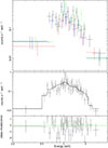 |
Fig. 10. Same as in Fig. 9 but for CP Pup. |
| In the text | |
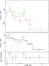 |
Fig. 11. Same as in Fig. 9 but for HZ Pup. |
| In the text | |
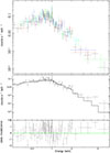 |
Fig. 12. Same as in Fig. 9 but for RR Pic. |
| In the text | |
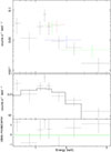 |
Fig. 13. Same as in Fig. 9 but for V407 Lup. |
| In the text | |
|
Fig. 14. Hardness ratio plot with our detected novae and simulated paths for spectral models with variable absorption hydrogen column (increasing between 1 × 10²⁰ and 2 × 1022 cm−2 from left to right). Pure thermal plasma models (mekal) are shown in dashed lines, with kT increasing from 1 keV (blue, dashed line) to 35 keV. All models with kT above 5 keV collapse on the same path on the plot (red dashed line). Dotted lines show models with an extra soft, blackbody component with effective temperatures from 20 eV (purple) to 90 eV (green). The simulations with a soft component also include a thermal plasma with kT = 15 keV and a normalisation of a factor 10 fainter than the blackbody. Detected historical novae in the eRASS:4 are shown as big dots for new detections, stars for known IPs, and triangles for all other cases. |
| In the text | |
|
Fig. B.1. AT Cnc contour plots for the spectral model parameters at 68%, 90%, and 99% confidence levels. From top left to bottom right: Absorbing hydrogen column (in units of 1022cm−2) vs blackbody (kT); blackbody normalization ( L39/D102, where L39 is luminosity in units of 1039erg/s and D10 is the distance in units of 10 kpc) vs blackbody (kT); and cooling flow normalization (mass accretion rate in units of M⊙yr−1) vs the lowest and highest plasma temperature of the cooling flow. |
| In the text | |
|
Fig. B.2. BD Pav contour plots for the spectral model parameters at 68%, 90% and 99% confidence levels. Absorbing hydrogen column (in units of 1022cm−2) vs cooling flow normalization (mass accretion rate in units of M⊙yr−1, left panel) and the highest plasma temperature of the cooling flow (right panel). |
| In the text | |
Current usage metrics show cumulative count of Article Views (full-text article views including HTML views, PDF and ePub downloads, according to the available data) and Abstracts Views on Vision4Press platform.
Data correspond to usage on the plateform after 2015. The current usage metrics is available 48-96 hours after online publication and is updated daily on week days.
Initial download of the metrics may take a while.