| Issue |
A&A
Volume 704, December 2025
|
|
|---|---|---|
| Article Number | A145 | |
| Number of page(s) | 16 | |
| Section | Extragalactic astronomy | |
| DOI | https://doi.org/10.1051/0004-6361/202556809 | |
| Published online | 05 December 2025 | |
Beyond diagnostic-diagrams: A critical exploration of the classification of ionization processes
1
Instituto de Astronomía, Universidad Nacional Autonóma de México, A.P. 106, Ensenada, 22800 BC, Mexico
2
Instituto de Astrofísica de Canarias, La Laguna, Tenerife E-38200, Spain
3
Departamento de Astrofísica, Universidad de La Laguna, Dpto. Astrofísica, 38206 La Laguna, Tenerife, Spain
4
Instituto de Radioastronomía and Astrofísica (IRyA-UNAM), 3-72 (Xangari), 8701 Morelia, Mexico
5
Instituto de Astrofísica de Andalucía (IAA-CSIC), Granada E-18008, Spain
⋆ Corresponding author: This email address is being protected from spambots. You need JavaScript enabled to view it.
Received:
11
August
2025
Accepted:
6
October
2025
Abstract
Context. Diagnostic diagrams based on optical emission lines, especially classical BPT diagrams, have long been used to distinguish the dominant ionisation mechanisms in galaxies. However, these methods suffer from degeneracies and limitations, particularly when applied to complex systems such as galaxies, where multiple ionisation sources coexist.
Aims. We aim to critically assess the effectiveness of commonly used diagnostic diagrams in identifying star-forming galaxies, retired galaxies (RGs), and active galactic nuclei (AGNs). We also explore alternative diagnostics and propose a revised classification scheme to reduce misclassifications and better reflect the physical mechanisms ionizing gas in galaxies.
Methods. Using a comprehensive sample of nearby galaxies from the NASA-Sloan Atlas (NSA) cross-matched with Sloan Digital Sky Survey (SDSS) spectroscopic data, we defined archetypal subsamples of late-type and star-forming galaxies, early-type and retired galaxies, and multiwavelength-selected AGNs. We evaluated their distribution across classical and more recent diagnostic diagrams, including the WHaN, WHaD, and a newly proposed WHaO diagram, which combine Hα equivalent width with additional indicators (N II/Hα, σHα and O III/O II, respectively). We carried out a quantitative comparison of the resulting classification across multiple schemes.
Results. Classical BPT diagrams systematically overestimate the number of star-forming galaxies (∼10%) and misclassify a significant fraction of AGNs (up to 45%) and RGs (up to 100%). Diagrams incorporating the equivalent width of Hα, such as WHaN, WHaD, or WHaO, yield more reliable separations (with ∼20% of AGNs and ∼15% of RGs erroneously classified). A new classification scheme based on EW(Hα) thresholds and concordant WHaD/WHaO results achieves an improved level of purity for all classes (with ∼8–25% sources erroneously classified) and a better alignment with known physical properties.
Conclusions. The widely used BPT-based classifications fail to accurately distinguish between ionisation mechanisms, especially in galaxies hosting low-luminosity AGNs or retired stellar populations. Updated schemes incorporating EW(Hα) and complementary diagnostics, despite their respective limitations, provide a more accurate view of galaxy ionisation and should be adopted in future studies of galaxy populations and evolution.
Key words: galaxies: active / galaxies: evolution / galaxies: ISM / galaxies: spiral
© The Authors 2025
 Open Access article, published by EDP Sciences, under the terms of the Creative Commons Attribution License (https://creativecommons.org/licenses/by/4.0), which permits unrestricted use, distribution, and reproduction in any medium, provided the original work is properly cited.
This article is published in open access under the Subscribe to Open model. This email address is being protected from spambots. You need JavaScript enabled to view it. to support open access publication.
1. Introduction
The interstellar medium (ISM) in galaxies can be ionized by a range of very different mechanisms associated with a variety of physical processes. According to Sánchez (2020), the most relevant ones are photo-ionization by (i) OB young and massive stars in recent star formation (SF) events (e.g., Strömgren 1939; Osterbrock et al. 1992), which comprises the classical H II regions; (ii) hot evolved low-mass stars (HOLMES) and post-asymptotic giant branch stars (p-AGB stars, e.g., Binette et al. 1994; Flores-Fajardo et al. 2011) observable in non-star-forming and retired galaxies (RGs) and regions within them (Singh et al. 2013; Belfiore et al. 2017; iii) active galactic nuclei (AGNs) produced by the gas accretion into central super-massive black holes in certain galaxies (Sandage 1965; Urry & Padovani 1995; iv) ionization produced by shocks at local or global scales, in particular, those in high-velocity galactic outflows from strong nuclear SF processes and/or AGNs (e.g., Veilleux et al. 2005; López-Cobá et al. 2019; v) optical jets in AGNs (e.g., López-Cobá et al. 2017; vi) low velocity outflows and inflows (e.g., Dopita et al. 1996; Kehrig et al. 2012; Roy et al. 2018); and (vii) supernovae remnants (e.g., Cid Fernandes et al. 2021). Low-velocity shocks and HOLMES and/or p-AGB ionization are observable only when the other ionizing processes are weak or absent, as the main ingredients of the diffuse-ionized gas (DIG) in RGs. On the contrary, in star-forming galaxies (SFGs), an additional important contribution to the DIG is produced by the photons that have leaked from H II regions (e.g., Sánchez et al. 2021; Belfiore et al. 2022; Lugo-Aranda et al. 2024).
Understanding the ionizing sources responsible for the excitation of the ISM in galaxies is critical not only to characterize the ISM itself, but also to make accurate estimations of key evolutionary tracers, such as the SF rate (SFR) and chemical abundance (for recent reviews, see Kewley et al. 2019; Sánchez et al. 2021). Optical spectroscopy, particularly the diagnostic line ratio diagram, has long served as the main tool to identify the dominant ionization mechanisms across galaxy populations. Among these, the Baldwin, Phillips, & Terlevich (BPT) diagram (Baldwin et al. 1981), which compares O III/Hβ and N II/Hα ratios, remains the most widely used. It is assumed that it effectively separates ionization by young massive OB stars in H II regions from harder ionization sources, such as AGNs and shocks, based on their differing line-ratio signatures (Osterbrock 1989; Veilleux et al. 2001).
Despite its utility, the classical BPT diagram (and others like it) faces significant limitations. First, the so-called “intermediate” or “composite” region between star-forming and AGN-dominated zones, defined by the demarcation lines of Kauffmann et al. (2003, hereafter K03) and Kewley et al. (2001, hereafter K01), can be populated by systems such as low-luminosity and/or metal-poor AGNs, supernova remnants (SNRs), and even pure star-forming regions (e.g., Cid Fernandes et al. 2021; Agostino & Salim 2019; Osorio-Clavijo et al. 2023). Second, evolved ionizing sources such as post-AGB stars or HOLMES can mimic AGN-like line ratios, even though their emission is intrinsically weaker. Shocks, of both high and low velocity, can also reproduce AGN-like signatures for particular gas properties, velocity, and magnetic field strength (e.g., Dopita et al. 1996; López-Cobá et al. 2020).
These poorly defined areas challenge the interpretation of diagnostic diagrams. In response, hybrid approaches have been introduced, such as the WHaN diagram (Cid Fernandes et al. 2010), which uses also the N II/Hα ratio and the equivalent width of Hα (EW(Hα)). Similar strategies have been proposed to clean star-forming sequences from RG contamination by incorporating EW(Hα) into traditional diagrams (Lacerda et al. 2018; Sánchez et al. 2014, 2018). However, even these improvements have limitations when emission lines are weak (e.g., in RGs), heavily dust-attenuated, or when the signal-to-noise ratio (S/N) is insufficient for all four lines required in BPT-style diagnostics. To overcome these issues, some authors have explored how the combination of the O III/Hβ line ratio with other suitable spectral features (such as D4000, g − r color, or the EW(Hβ)) can effectively discriminate between different ionizing sources (e.g., Teimoorinia & Keown 2018; Muñoz Santos et al. 2025). Finally, Sánchez et al. (2024) introduced an even more simple method, the WHaD diagram, that combines two parameters (EW(Hα) and σHα) both derivable from a single emission line. These methods significantly simplify the classification of ionizing sources.
All diagnostic diagrams are in practice validated using observational data (e.g., K03) or theoretical models (e.g., K01). In essence, the distribution of known/assumed line parameters, of galaxies and/or regions within them whose ionization is clearly known, defines a region within the diagram. The classification procedure is validated depending on how clearly the regions associated with different physical processes are separated. This approach was followed by most studies proposing a new diagnostic diagram and a boundary or demarcation line to separate different ionizing sources (e.g., Baldwin et al. 1981; Veilleux & Osterbrock 1987; Osterbrock 1989; Kauffmann et al. 2003; Kewley et al. 2001; Cid Fernandes et al. 2011; Sánchez et al. 2024).
There is a fundamental limitation in this method, as it relies on precise knowledge of the ionization mechanism responsible for the observed or modeled properties. Consequently, when validating against observational data, it is necessary to assume a specific ionizing source, which tends to be an OB star linked to recent SF. On the other hand, theoretical models demand the assumption of complete understanding of the underlying physical processes, the nature of the ionizing sources, and the characteristics of the ionized gas. Furthermore, using the available data, it has been assumed that only one mechanism is present, which is intrinsically impossible in complex systems such as galaxies (e.g., Sánchez 2020; Sánchez et al. 2021). Finally, there are degenerancies between different mechanisms that could produce the same observational properties (e.g., line ratios). The ionization strength versus metallicity degenerancy is one of the best known ones (e.g., K01, Sánchez et al. 2015), but there are many others that are not frequently considered (e.g., the post-AGB-shocks-AGN degenerancy described above). The use of spatial resolved information that allows to explore the morphology of the ionized gas, its kinematics, and even the properties of the underlying continuum (stellar or not) is a much better method to provide an optimal classification of the ionizing mechanism (Sánchez 2020; Sánchez et al. 2021). However, this is not possible when single aperture spectroscopy is analyzed, as in most large galaxy surveys (e.g., SDSS, DESI York et al. 2000; Levi et al. 2019).
The aim of this study is to perform a critical exploration of how we interpret some of the most frequently used diagnostic diagrams (and some others recently introduced) of galaxies in the nearby Universe extracted from the NSA catalog (Blanton et al. 2011). We selected a set of subsamples meant to be archetypal of SFGs, RGs, and galaxies hosting an AGN. We acknowledge that the ionization mechanisms present on each of those galaxy types may not be sharply defined (as indicated before). However, this is indeed part of the problem to be explored, as these diagrams are frequently used to distinguish between those groups without taking into account the real mixed nature of the ionization that produces the observed properties.
This article is organised as follows. Section 2 presents the datasets and galaxy samples employed in this study, including the different AGN selections and additional parameters used. The analysis of the data is presented in Sect. 3. It includes the qualitative description of the distributions of late-type galaxies (LTGs) and early-type galaxies (ETGs) in Sect. 3.1, alongside the diagnostic diagrams explored, in contrast with that of the AGN hosts (Sect. 3.2). A quantitatively study of how the archetypal subsamples are classified using different schemes is included in Sect. 3.3. Finally, we discuss how the full sample would be classified when using those very same schemes, including our newly proposed one is presented in Sect. 3.4. In Sect. 4, we present the results, including a revision of the methods adopted to select the AGNs in this study in the light of our own results (Sect. 4.1), and a sanity check of how we could reproduce some well established results when adopting our proposed classification scheme (Sect. 4.2). Finally, we present the conclusions in Sect. 5. We assumed a standard Λ cold dark matter cosmology with parameters: H0 = 71 km s−1 Mpc−1, ΩM = 0.27, ΩΛ = 0.73, in concordance with Sánchez et al. (2022).
2. Data
2.1. Galaxy sample and spectroscopic data
We extracted our sample of galaxies from version v1_0_1 of the NSA dataset1 (Wake et al. 2017), which is a catalog of parameters of ∼600 000 nearby galaxies (z < 0.3) selected from the Sloan Digital Sky Survey (SDSS York et al. 2000). It includes improved photometric measurements in the SDSS ugriz bands, as well as far- and near-ultraviolet photometry (FUV and NUV, respectively) provided by the Galaxy Evolution Explorer (GALEX; Martin et al. 2003). It also includes additional parameters, such as the redshift of the target, structural and morphological information, and additional quantities such as the stellar masses, new derivation of the Sérsic indices, and new aperture corrections applied to all photometric values accounting for the PSF differences between filters.
Additional spectroscopic information can be obtained for each galaxy in the NSA by looking for the corresponding target listed in the catalog of galaxy properties for SDSS-DR8 (Aihara et al. 2011) derived using the MPA-JHU analysis2. Among the extracted information, the most relevant for the current exploration are the flux, equivalent width, and velocity dispersion from the O III, N II, S II, O I, Hα, and Hβ emission lines. Although there are more recent analyses of the same dataset, this one has been broadly used in relevant explorations such as the uncovering of the mass-metallicity relation (Tremonti et al. 2004), the star-forming main sequence (Brinchmann et al. 2004), as well as the seminal exploration of the distribution of galaxies in the BPT diagrams by K03. We applied a cut in the redshift to exclud the galaxies in the local volume (z > 0.005) and maximizing the completeness of the NSA catalog (z < 0.1). The cross-matched catalog (hereafter, NSA-MPA-JHU, or NMJ sample) comprises a total number of 545 548 galaxies, including all galaxy types and covering a wide range of stellar masses. This sample could be considered by all means representative of the population in the Local Universe (once dwarf galaxies have been excluded) and it is one of the largest samples of galaxies with spectroscopic information available to date within the considered redshift range.
2.2. AGN samples
The selection of bona-fide AGNs to validate the classification using different diagnostic diagrams is a difficult task. Thus, different approaches have been adopted in the literature. For instance, Sánchez et al. (2024) used two samples of X-ray-selected AGNs (X-AGNs) from Osorio-Clavijo et al. (2023) and Agostino & Salim (2019), under the assumption that the X-ray emission is a reliable tracer of the nuclear activity. However, this might bias the results toward a particular type of objects, so, we preferred to follow Comerford et al. (2020) and select a sample of AGNs based on different selection criteria, including X-ray, infrared (IR), UV-optical, and radio selections.
2.2.1. X-AGNs
The sample of X-AGNs was extracted from the 4XMM-DR14s catalog3 (Traulsen et al. 2020). This is a comprehensive compilation of serendipitous X-ray sources detected by the XMM-Newton observatory and it covers a wide area on the sky. The catalog includes 427 524 sources, of which 329 972 have been observed multiple times. In total, it lists over 1.8 million individual flux measurements across the standard XMM-Newton energy bands (0.2–12.0 keV). For each source, parameters such as flux, hardness ratio, and variability indicators are provided. The size, spatial coverage, and unbiased selection criteria make this sample suitable for the current exploration.
We cross-matched the 4XMM-DR14s catalog with our NMJ sample of galaxies, looking for coordinates matching within 3″ (i.e., the size of the SDSS fiber). We found a total of 1390 coincidences, from which we assign the X-ray properties in the catalog to the corresponding NSA galaxies. For each galaxy, we derived (i) the X-ray luminosity (LX) in the hard band (2–12 keV), using the redshift included in the catalog, along with (ii) the hardness ratio (HR), defined as
 (1)
(1)
where H corresponds to the flux in the X-ray hard band and S corresponds to the soft band (0.2–2 kev).
The X-AGNs candidates are characterized by LX > 1041 erg s−1 and HR > −0.2. It is known that a cut in luminosity of 1042 erg s−1 minimizes the contamination from any ionizing source different than an AGN (e.g., Brightman & Nandra 2011). However, it could exclude a considerable fraction of AGNs as well (e.g., Osorio-Clavijo et al. 2023). Lowering the luminosity limit by an order of magnitude would increase the possible contamination of other ionizing sources (e.g., SF) by just a 3%. Finally, we imposed a cut in HR to select only the X-AGNs with the hardest radiation (e.g., Melnyk et al. 2013), which is particularly effective for selecting obscured targets. Adopting these criteria, we ended up with 627 X-AGNs.
2.2.2. IR selected AGNs
The all-sky imaging survey performed by the Wide-field Infrared Survey Explorer (WISE Wright et al. 2010) in four bands centered at 3.4 μm, 4.6 μm, 12 μm, and 22 μm (hereafter referred to as W1, W2, W3, and W4) was used to define a sample of IR-selected AGNs (I-AGNs). We performed a positional crossmatch between the NMJ catalog and the WISE catalog using a matching radius of 6″, the typical PSF FWHM (for the shorter WISE wavelength bands). Almost all targets in our NMJ catalog match with a WISE target (i.e., 541 478 matched sources). For these objects, we adopted the profile-fit magnitudes provided by the AllWISE catalog. There are multiple WISE-based color-selection methods available for selecting AGNs (e.g., Wright et al. 2010; Jarrett et al. 2011; Donley et al. 2012; Assef et al. 2018; Comerford et al. 2020). We followed Assef et al. (2018) and Comerford et al. (2020), as they perform an exploration somehow similar to the one attempted here. We adopted a criterion based on two different color cuts for two different IR brightness ranges:
 (2)
(2)
This method yields a sample of 7871 I-AGNs.
2.2.3. UV/optical photometry selected AGNs
We used the UV and optical photometry included in the NSA catalog and selected candidate AGNs based on the color distributions shown by Trammell et al. (2007). We applied the following criteria: (i) NUV − u < 2 mag; (ii) NUV − g < 4 mag; (iii) FUV − NUV < 0.5 mag; (iv) u − g < 0.6 mag; and (v) g − r < 0.6 mag. An additional cut has been included in the absolute magnitude of the UV bands to exclude intrinsically faint targets (FUVabs < −19.5 mag and NUVmag < −18 mag). We should note that some of these criteria are somehow redundant and the most restrictive ones are those including the NUV − u and u − g colors. A total of just 330 objects were selected using this rather restrictive criterion, tracing essentially unobscured AGNs (O-AGNs hereafter). The low number of recovered O-AGNs is due to the selection criteria, which was tuned to select QSOs: AGNs with a negligible contribution from the host galaxy (in contrast to the objects in our NMJ sample).
2.2.4. Radio-selected AGNs
We used the Faint Images of the Radio Sky at Twenty centimeters radio survey (FIRST Becker et al. 1995) to identify a sample of radio AGNs (R-AGNs) in the NMJ catalog. FIRST has observed 10 000 square degrees of both hemispheres at 1.4 GHz, generating a catalog of one million sources. Following the same procedure described in Sect. 2.2.2, we cross-matched their position in the sky with that of our main galaxy sample, looking for coincidences within the same distance as the one adopted for selection of I-AGNs. We found a good match for 18 851 galaxies. From these, we selected the brightest and clearly resolved targets by imposing the following criteria: (i) a minimum integrated flux of 10 mJy; (ii) a minimum FWHM along the major axis of 0.5″; and (iii) that the integrated flux is at least 1.1 larger than the peak flux (following Ivezić et al. 2002). These criteria minimize the possible contamination by star-forming galaxies that may present emission in the radio continuum, being usually fainter and more compact (e.g., Wadadekar 2004). Similar criteria have been adopted in the literature to select extended radio sources (e.g., Kimball et al. 2011). Following this procedure, we selected a final sample of 1098 R-AGNs.
2.3. Final galaxy and AGN sample
In summary, we compiled a catalog of more than half a millon galaxies, comprising photometric, structural and spectroscopic properties, together with positions on the sky, redshift, and distance, by combining the NSA and MPA-JHU catalogs, which we call the NMJ sample. In addition, we have created four samples of AGNs by (1) cross-matching NMJ with the 4XMM-DR14s catalog of X-ray sources, then applying a cut in luminosity and hardness ratio (X-AGNs; Sect. 2.2.1); (2) cross-matching NMJ with the AllWISE catalog of IR sources, then applying a cut in the IR colors depending on the brightness of the targets (I-AGNs; Sect. 2.2.2); (3) selecting objects with a clear UV/blue color excess (O-AGNs; Sect. 2.2.3); and (4) cross-matching the NMJ sample with the FIRST catalog of radio sources, applying an absolute and relative threshold in their extended fluxes and their projected size (R-AGNs; Sect. 2.2.4). Table 1 lists the number of objects included in the NMJ catalog and the result of cross-matching with each of the multiwavelength catalogs described earlier in this work (XMM, WISE, UV/Optical, and FIRST), together with the number and fraction of AGNs selected using those datasets. The total number and fraction of AGNs selected when combining the four methods is listed as well.
Number of galaxies and AGNs in the analyzed sample.
2.4. Additional parameters
The combination of the NMJ catalog with the XMM, WISE, and FIRST datasets provides a large sample of galaxies with a wide set of physical properties. For the purpose of this work, we derived two additional parameters to characterize the explored galaxies: the disk fraction and the integrated SFR.
2.4.1. Disk fraction (fdisk)
It is relevant for our exploration to understand whether or not a galaxy presents a prominent disk. We used the fact that disk-dominated LTGs and bulge-dominated ETGs are located in different regions of the effective radius (Re) versus stellar-mass M⋆ plane (e.g., Shen et al. 2003; van der Wel et al. 2014; Lange et al. 2015), defining the disk fraction, fdisk. This can be expressed as
 (3)
(3)
where Re,LT and Re,ET are the effective radius of the stellar mass predicted by Shen et al. (2003) for LT and ET galaxies, respectively. As a proxy of Re we adopted the ELPETRO_THETA_R parameter in the NSA catalog, transformed to kpc using the angular distance estimated using the standard cosmology and the redshift provided by the same catalog. Finally, we used SERSIC_MASS in the NSA for M⋆
We stress that fdisk should not be taken as a detailed estimation of the real fraction of disk (or bulge) in luminosity or mass in a galaxy. However, it does provide a simple and robust method to segregate between disk-dominated and bulge-dominated galaxies. Furthermore, it does not require a detailed profile fitting (e.g., Sérsic index), neither does it rely on a discrete morphological classification.
2.4.2. Integrated SFR
The MPA-JHU catalog provides different estimations of the SFR. However, all of them rely on the spectroscopic information, in particular, the Hα flux, which is biased to the central regions sampled by the SDSS fibers; thus, it may not be representative of the SF status of the entire galaxy (e.g., González Delgado et al. 2016; Sánchez et al. 2018). To obtain an independent and robust estimation of the integrated SFR that takes into account the dust obscuration, we used the UV and IR photometry provided by the GALEX and WISE datasets. Then, we adopted the calibrators proposed by Cluver et al. (2017) and Catalán-Torrecilla et al. (2015) to estimate the SFR based on the 12μ and 22μ WISE photometry. We averaged them to obtain a single estimation for the SFR using the two IR bands (SFRIR). Then, we adopted Catalán-Torrecilla et al. (2015) calibrators to estimate the SFR using the GALEX FUV (SFRUV) and the final SFR resulting from the combination of both SFRIR and SFRUV.
Figure 1 shows a comparison between the SFR derived using this method and the values reported by the MPA-JHU for this parameter (SFR_tot_p50 in that catalog) for the full NMJ sample analyzed along this study. Although there is a relatively good correlation between both estimations in the range of high values (following almost a one-to-one relation) the MPA-JHU reports a wider range of SFRs, with a clear trend to much lower values, in particular in the range of low values. This is exactly what would be expected when extrapolating the Hα emission in the center of galaxies toward their entire extensions based on a limited aperture for intermediate type galaxies (early spirals) such as Sa/Sb morphologies, as indicated before. Additional differences are expected as the timescale of the SF sampled by the different indicators (Hα vs. IR/UV) is intrinsically different (e.g., Kennicutt 1983). When required, we used the M⋆ parameter described in the previous section, together with the derived SFR to obtain the specific SFR (sSFR = SFR/M⋆).
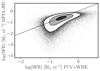 |
Fig. 1. Comparison between the SFR provided by the MPA-JHU catalog and the one derived combining the IR and UV photometry as described in the text. The black dots correspond to each galaxy in the NMJ sample (i.e., the full sample of galaxies analyzed in this article) and each successive grey contour represents the area encircling a 90%, 65%, and a 15% of these points. The dashed-line represent the one-to-one relation. |
3. Analysis
As indicated in the introduction, our aim is to determine whether or not the three groups in which we divide galaxies according to their main ionization mechanism (SFGs, RGs, and AGNs) are located in well defined regions in a set of diagnostic diagrams. With this purpose in mind, it is important to select three subsamples of galaxies trying to limit as much as possible any possible contamination by the ionization dominating the other subsamples. Furthermore, to avoid as much as possible circular arguments, in this selection we describe the galaxy properties that were not explored in the diagnostic diagrams.
For AGNs, we simply adopted the four subsamples described in the previous sections, as all of them fulfill the previous requirements. As an archetypal subsample of SFGs, we selected blue (u − g < 2) LT galaxies (nsersic < 1.5), without any evidence of a bulge (fdisk > 0.85), and clearly located in the SF main sequence (SFMS, e.g., Brinchmann et al. 2004; Renzini & Peng 2015); namely, with log(sSFR) > –11.5 dex (following Sánchez et al. 2019). With the additional criterion that the Hα flux has a S/N > 3, this subsample of essentially LT galaxies consists of 90 076 objects. On the contrary, our subsample of non-star-forming galaxies were selected as red (u − g > 2), ET galaxies (nsersic > 3.5), without any clear evidence of a disk (fdisk < 0.05), and well below the SFMS (sSFR < –11.5 dex). Considering a similar minimum S/N in the Hα flux the subsample of early-type galaxies (ETGs) comprises 43 295 objects4.
3.1. LTGs and ETGs across the diagnostic diagrams
Figure 2 shows the distributions along a set of diagnostic diagrams for the entire sample of NMJ galaxies and the subsamples of LTGs, ETGs, and X-AGNs defined before, together with the boundaries defining regions associated with different physical processes. The top panels correspond to the classical BPT diagrams (Baldwin et al. 1981; Veilleux et al. 2001) that present the distribution of the O III/Hβ line ratio as a function of N II/Hα (BPT-N2), S II/Hα (BPT-S2) or O I/Hα (BPT-O1). The bottom panels include three diagnostic diagrams that represent the equivalent width of Hα, EW(Hα), along N II/Hα (WHaN, Cid Fernandes et al. 2010), the Hα velocity dispersion (WHaD, Sánchez et al. 2024), and the O III/O II line ratio (WHaO diagram, hereafter). As already discussed in Sect. 1, all diagrams attempt to segregate between the ionization associated with recent SF and AGN. In addition, the diagrams using EW(Hα) include a new category with the ionization associated with retired galaxies (Ret.). Those diagrams distinguish between strong AGNs (sAGNs, EW(Hα) > 6 Å) and weak AGNs (wAGNs, EW(Hα) < 6–10 Å) too. For a more simple comparison with the classification performed using the BPT diagrams, we did not distinguish between both sub-categories of AGNs and discuss them together. Finally, there are diagrams in which a certain region is labeled as mixed+composite or with an unknown ionization source. For simplicity, we considered all those galaxies together in a single category labeled as Mix/Unk. Each diagram shows on top the D parameter derived from a set of 2D Kolmogorov-Smirnov (KS) tests comparing the distribution of LTGs versus ETGs (L/E), ETGs versus X-AGNs (E/A), and LTGs versus X-AGNs (L/A). The D parameter from a KS-test is near zero when the two samples are derived from the same parent sample, and it is near one when derived from different parent samples. Thus, a value close to zero (one) means that the two samples are indistinguisable (clearly distinguisable). The significance of these tests is in general better than 1%, due to the large number of objects considered in each subsample. Similar distributions for the other three subsamples of AGNs described in Sect. 2 are included in Appendix A.
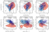 |
Fig. 2. Distribution of the subsamples of galaxies across different diagnostic diagram. Top panels: Classical BPT diagrams (Baldwin et al. 1981), showing the distribution of O III/Hβ line ratio as a function of N II/Hα ratio (left panel), S II/Hα (middle panel), and O I/Hα (right panel). Solid and dot-dashed lines correspond to the demarcation lines proposed by K03 and K01 to distinguish between the different ionizing sources. Bottom panels: Diagrams comparing the distribution of Equivalent-width of Hα (WHα) as a function of (i) the N II/Hα ratio (left panel) WHaN diagram (Cid Fernandes et al. 2010; ii) the Hα velocity dispersion (σHα, middle panel), WHaD diagram (Sánchez et al. 2024); and (iii) the O III/O II line ratio (right panel), proposed here as the WHaO diagram. In each panel, the black dots correspond to the full NMJ sample and each successive grey contour represents the area encircling the 90%, 65%, and a 15% of these points. The blue (red) contour represent the area that encircles 90% of the values corresponding to the LT (ET) subsamples of galaxies, as defined in the text. Finally, the location of the X-ray-selected AGNs are shown as dark-blue stars. The D parameter derived for a set of 2D KS-tests comparing the distributions of the different subsamples are included on top of each panel, using the nomenclature L/E when comparing LTGs versus ETGs, E/A for ETGs versus X-AGNs, and L/A for LTGs versus X-AGNs. |
The WHaO is a new diagram5 that has been introduced following a similar reasoning used in the WHaN and WHaD diagrams, comparing two parameters that trace two different physical properties associated with different ionization mechanisms: (i) the EW(Hα) traces the relative strength of the Hα emission line with respect to the continuum level. High (absolute) values are found in either galaxies under SF or hosting an AGN, while low values are observed when neither SF nor strong AGNs are present; and (ii) the O III/O II ratio, frequently used to estimate the ionization parameter (U, e.g., Dors et al. 2011; Sánchez et al. 2015; Espinosa-Ponce et al. 2022), but actually tracing the hardness and shape of the ionizing spectrum better (Morisset et al. 2016). The harder the ionizing spectrum (e.g., in the case of post-AGB stars and AGNs), the larger this parameter should be.
The distributions along the different diagrams agree to the expectations and the previous knowledge (e.g., Sánchez 2020). If we focus on the BPT-N2 diagram, it is clear that LTGs are found in the classical location of HII regions (e.g., Osterbrock 1989), following the left-branch of the well-known V-shaped distribution for the entire galaxy sample. However, they present a slight shift toward the so-called mixed/intermediate region, between the K03 (dot-dashed) and K01 (solid) demarcation lines. Similar distributions are seen, to some extent, in the other two BPT diagrams, with a stronger shift toward regions of higher S II/Hα and O I/Hα line ratios, slightly overpassing the K01 demarcation line (this does not happen in the BPT-N2 diagram).
On the other hand ETGs are distributed following mostly the right-branch of the full galaxy distribution in the BPT-N2 diagram. They cover a wide range of line ratios that expands from the location classically assigned to strong AGNs (at the upper-right end of the diagram), crossing the so-called intermediate+mixed regime and expanding clearly within the right-end of the distribution classically associated with ionization related to SF (i.e., the location of where H II regions are located, e.g., Sánchez et al. 2015; Espinosa-Ponce et al. 2020; Lugo-Aranda et al. 2024). This pattern is repeated in the other BPT diagrams (BPT-S2 and BPT-O1), clearly illustrating that none of those diagrams was defined (and therefore their are not useful) to perform a segregation between RGs and SFGs (as already noted in the literature; e.g., Sánchez 2020; Sánchez et al. 2021, and references therein).
The diagrams that use EW(Hα), (lower panels of Fig. 2) segregate much better LTGs from RGs. Among the parameters used to select both subsamples we adopted the sSFR, that would be a tracer of EW(Hα) if it were estimated using the SFR derived from the Hα luminosity (Sánchez et al. 2014; Belfiore et al. 2017) and the data obtained within the same aperture. For this reason we adopted a different calibrator to estimate the SFR (Sect. 2.4). Furthermore, we note that the separation, although it is driven by EW(Hα), it is somehow observed in the second parameter adopted for each of these diagrams. Thus, on average, LTGs present lower σHα, lower N II/Hα ratios and lower O III/O II ratios than ETGs. This is expected. First, the ionized gas in disk dominated galaxy should present a lower velocity dispersion than that observed in a bulge dominated one. Second, in the case of the line ratios, a high ionization parameter and a hard ionizing radiation field produce higher values of both line ratios (Stasińska et al. 2015), being more typical of the ionizing sources present in ETGs. However, in the case of ionizing sources associated with LTGs for low metallicities and in the presence of density-bounded H II regions, while the N II/Hα ratio remains low, high values of O III/O II have been reported (e.g., Overzier et al. 2009; Kewley et al. 2013; Jaskot & Oey 2013; Stasińska et al. 2015). Thus, the first of these two line ratios seem to perform a better segregation between LTGs and ETGs than the WHaO diagram.
The 2D KS-tests carried out for each diagram confirm the results outlined before. For any of the BPT diagrams, the D parameter resulting from the comparison of the distributions of LTGs and ETGs is smaller than the value found for any of the diagrams that use EW(Hα). For the diagrams in the top panel of Fig. 2, the largest reported value is 0.79 (BPT-N2 diagram), while for the diagrams in the bottom panel, the smallest value is 0.92 (WHaO diagram).
3.2. AGNs across the diagnostic diagrams
Once established which are the preferred location of LTGs and ETGs in the diagrams, we explore which areas are occupied by our sample of AGNs. Again, we start with the BPT-N2, the most commonly used diagram to select AGNs using optical spectroscopic data. The first obvious result from a visual exploration is that X-AGNs are clearly not confined to the usual region classically assigned to this kind of ionization. Although a considerable number are located about the K01 demarcation line in this diagram, their distribution mimics that of the ETGs, spanning through a wide range of line ratios, from high N II/Hα and O III/Hβ values, to moderate N II/Hα and low O III/Hβ ones. X-AGNs are found not only below the K01 curve, but also below the most stringent K03, clearly invading the location occupied by our sample SFGs (i.e., the classical location of H II regions). This pattern is not only observed in the BPT-N2 diagram, it is also in the other two BPT diagrams, with a larger degree of overlapping between the X-AGNs and LTGs. Osorio-Clavijo et al. (2023) already showed a similar result for a limited sample of well selected X-AGNs. We should note that, like in the case of this study, the distribution of X-AGNs toward regions below the classical demarcation lines is not correlated with the X-ray luminosity. In Fig. 2, we coded the size of the figure by this luminosity, showing that even the most luminous X-ray sources could be located in the area below both demarcation lines (K01 and K03).
The distribution of X-AGNs in the diagrams including EW(Hα) provide a better separation between LTGs and ETGs. In the case of LTGs, the separation is driven mostly by the second parameter included in the diagram (i.e., N II/Hα, σHα, or O III/O II). For ETGs, the separation is driven by EW(Hα) (in WHaN and WHaD) or by both parameters (in the new WHaO diagram). Certainly, there is no clear coincidence between the footprints of X-AGNs and ETGs found for the three BPT diagrams.
As in the case of the segregation between LTGs and ETGs, presented in Sect. 3.1, the 2D KS-tests comparing the distributions of those two subsamples of galaxies with the distribution of X-AGNs, confirm the main results presented above. For any of the BPT diagrams the D-value resulting from the comparison of the distributions of ETGs and X-AGNs is considerably smaller (∼0.32–0.44) than the value found for any of the diagrams that use EW(Hα) (∼0.75–0.77). On the other hand, for LTGs, only the BPT-N2 diagram presents a D-value (0.73) similar to the one of the diagrams using EW(Hα) (∼0.66–0.78). Finally, the results from the KS-tests indicate that X-AGNs are less clearly distinguished from LTGs and ETGs tham both galaxy samples between themselves (LTGs vs. ETGs): in all diagrams the values reported for the D parameters for the E/A and L/A cases are smaller than the ones reported for the L/E case.
Similar results are found when exploring the distributions of the other three AGN samples described in Sect. 2 (figures are included in Appendix A), with some significant differences: (i) in all cases, AGNs are not confined in the region classically assigned to these objects in the BPT diagrams, with I-AGNs and R-AGNs covering a region similar to X-AGNs, and O-AGNs being located mostly below the K01 demarcation lines in three BPT diagrams; (ii) I-AGNs trace better the classical loci assigned to Seyfert-II galaxies in the BPT diagram (e.g., Kewley et al. 2006), while R-AGNs present lower O III/Hα values for a given N II/Hα, S II/Hα, or O I/Hα ratio, tracing the region usually assigned to LINERs (Heckman 1987). In both cases the distribution crosses the K01 (and K03) demarcation line invading the area associated to SF ionization; (iii) regarding the diagrams including EW(Hα) both I-AGNs and R-AGNs follow a somehow similar pattern as the one described for the X-AGNs, with a significantly larger number of R-AGNs located in the area covered by ETGs (in agreement with their distribution in the BPT diagrams), and a larger number of R-AGNs found in the area assigned to SF related ionization in the WHaO diagram; finally; (iv) O-AGNs are located in the same region covered by X-AGNs only for the WHaD and WHaO diagrams, but not for the WHaN one. These differences reflect the different kind of AGN activity traced when applying different selection criteria.
3.3. Quantifying how well the ionization is classified
In Sect. 3.1, we explore the distribution of the three samples of galaxies (LTGs, ETGs, and AGNs) in a set of diagnostic diagrams. Here, we quantify how well the ionization can be classified based on these diagrams using these three samples as proxies. To do so, we adopted the following classification schemes:
-
(i)
BPT-N2: It is the most frequently adopted scheme in the literature. It uses the location across the BPT diagram using the N II/Hα ratio to classify galaxies as SFGs (below the K03 curve), mixed or unknown (above the K03 curve and below the K01 one), and AGNs (above the K01 curve). This scheme is not able to select RGs by construction.
-
(ii)
BPT-ALL: Defined by the location across the three BPT diagrams, classifying the galaxies as SFGs if they lie below the K01 curve in each diagram, AGNs if the lie above the same curves in all diagrams and mixed/uknown if the do not fulfill any of the two criteria. This method is more restrictive than the previous one for AGNs, but not for SFGs. As in case of the BPT-N2 method, the RGs type is not considered by this classification procedure.
-
(iii)
BPT-N2+WHa: It uses the BPT-N2 diagram combined with a cut in EW(Hα). This method was introduced by Sánchez et al. (2014), and discussed extensively in Sánchez (2020) and Sánchez et al. (2021), as a method to select RGs (following Stasińska et al. 2008; Cid Fernandes et al. 2011), while retaining the information provided by the classical BPT diagrams. Galaxies are classified as RGs if EW(Hα) < 3 Å, irrespective of their location within the BPT-N2 diagram. They are classified as SFGs (AGNs) if they are located below (above) the K01 curve and EW(Hα) > 6 Å. Galaxies not fulfilling any of the previous criteria would be classified as mixed or unknown.
-
(iv)
WHaN: Galaxies are classified as RGs in a similar way as the previous method (i.e., EW(Hα) < 3 Å). For the remaining classes, we consider them SFGs (AGNs) if N II/Hα < 0.4 (> 0.4). This scheme is essentially the same as the one originally proposed by Cid Fernandes et al. (2011) for this diagram, with the only difference that it does not separate between weak and strong AGNs.
-
(v)
WHaD: RGs are selected in a similar way as in the previous scheme, purely based on the value of EW(Hα). However, SFGs are separated from AGNs based on the velocity dispersion of the Hα emission line, using a threshold of 57 km s−1 as the maximum value for star-forming galaxies. On the contrary to the previous method galaxies with σHα below this limit and intermediate EW(Hα) (3–6 Å) have undefined ionization (unknown or mixed), following Sánchez et al. (2024).
-
(vi)
WHaO: RGs are selected in a similar way as in the two previous cases. The SFGs (AGNs) are selected as non-RGs that present a O III/O II ratio lower (higher) than 0.63 (–0.2 dex in logarithm scale). As in the previous, case non-RGs and non-AGNs with an intermediate value for EW(Hα) are labeled as unknown or mixed.
-
(vii)
WHaDoO: It combines the WHaD and WHaO diagnostic criteria. First, RGs are selected using the same procedure described for those methods. Then galaxies are classified as AGNs if they fulfill the criteria for being this type based on any of the two schemes (i.e., WHaD or WHaO). Finally, galaxies are classified as SFGs if they are non-RGs, non-AGNs, and SFGs in both diagrams simultaneously. When galaxies do not fulfill any of the criteria they are labeled as unknown or mixed.
-
(viii)
WHaDaO: It is a variant of the previous method in which a galaxy is classified as AGN if it fullfill this criteria using both the WHaD and WHaO schemes. On the contrary, SFGs are selected as galaxies that are classified as this type in any of these two schemes.
-
(ix)
WHaD+O: It is a selection scheme developed based on the results of the current analysis, in which RGs are selected in a similar way as any of the previous schemes using EW(Hα). Finally galaxies are labeled as SFGs (AGNs) if they are classified this way using both the WHaD plus WHaO diagram. The remaining galaxies are classified as unknown or mixed.
Using these nine criteria we quantify how the galaxies on our initial archetypical subsamples (LTGs, ETGs, X-AGNs, I-AGNs, O-AGNs, and R-AGNs) are classified in the four different categories (SFGs, Mixed or unknown, RGs, and AGNs). The result is presented in Fig. 3, where we show the percentage of each type of galaxy classified in each ionization category according to the described classification schemes. For instance LTGs, a sample of galaxies that, by construction, were selected to present recent SF are preferably classified as SFGs. However, there are clear quantitative differences depending on the method. For instance, the BPT-N2 and the WHaDaO method locate most LTGs in the SFGs group (∼95%). On the contrary, the WHaDoO method is the one that assigns a lower number of LTGs to this group (∼74%). As expected no method classifies a substantial number of LTGs as retired (< 1%). The number of LTGs classified as AGNs is also low for the schemes using the BPT diagrams (∼1–4%). The percentage increases when a single diagram based on EW(Hα) (∼11–13%) is used, with the largest fraction being assigned by the WHaDoO method (∼23%). Finally both the WHaDaO and WHaD+O methods assign a very small fraction of LTGs to the AGN group (∼1%), providing with very similar results as the schemes using the BPT diagrams in this regards. The main difference between these two methods is that the latter one assigns a large number of LTGs to the unknown or mixed group (∼25%).
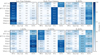 |
Fig. 3. Differences found in the classification of the dominant ionization when using different diagnostics. Each panel comprises a heat-map showing the fraction of objects (color scale and values within each cell) assigned to each type of ionization by a different diagnostic diagram for a different subsample of galaxies (from the top left to bottom right): LTGs, ETGs, X-ray-selected AGNs (X-AGNs), IR-selected AGNs (I-AGNs), UV-optically selected AGNs (O-AGNs), and radio-selected AGNs (R-AGNs). Each heat-map column corresponds to the different ionizing types considered in this work, namely: (i) ionization associated with recent SFGs; (ii) mixed or unknown ionization (Mix/Unk); (iii) ionization usually found in non-star-forming and retired galaxies (RGs), due to hot evolved stars (Binette et al. 1994; Flores-Fajardo et al. 2011), and/or low-velocity shocks (Dopita et al. 1996); and (iv) ionization associated with AGNs and or shocks associated with galactic scale winds (e.g., López-Cobá et al. 2020). On the other hand, each row corresponds to a different diagnostic scheme, including the use of: (i) the classical diagram by Baldwin et al. (1981) that uses O III/Hβ and N II/Hα line ratios (BPT-N2); (ii) the three diagrams by Baldwin et al. (1981) that use the O III/Hβ vs. N II/Hα S II/Hα and O I/Ha line ratios (BPT-all); (iii) the BPT-N2 diagram including a cut in the equivalent width of Hα (BPT-N2+WHa), as described in Sánchez (2020); (iv) the WHaN diagram that uses the N II/Hα and the equivalent width of Hα (WHaN); (v) the diagram introduced by Sánchez et al. (2024) that uses N II/Hα and the velocity dispersion of Hα (WHaD); (vi) the new proposed diagram that uses O III/O II and the equivalent width of Hα (WHaO). Finally, we have three different combinations that use the WHaD and WHaO diagrams: (vii) WHaDoO, (viii) WHaDoO, and (ix) WHaD+O, as described in the text. |
Larger differences are found in how each method classifies ETGs in different ionization types. By construction, these methods that do not incorporate EW(Hα) do not recover RGs by construction. Both, BPT-N2 and BPT-ALL, classify ETGs mostly as AGNs (∼65–72%), mixed or unknown (∼18–28%), and SFGs (∼7–11%). Those schemes that use EW(Hα) classify most ETGs as RGs (∼85–88%), with a very low number as SFGs (< 4%). The fraction of them classified as AGNs or without a clear classification is rather similar, ranging from ∼0% to ∼14%, depending on the method.
For the different subsamples of AGNs, we find significant differences, however we recover quantitatively the same patterns already described in our qualitative analysis. For X-, I- and R-AGNs, those methods that incorporate the BPT diagrams recover between ∼30% (for R-AGNs) and ∼69% (for I-AGNs), with ∼50% on average. The fraction of those AGNs without a clear classification (mixed or unknown), or even classified as SFGs, could be as large as ∼45%. On the contrary, the methods that adopt a single diagram involving EW(Hα) (WHaN, WHaD, and WHaO) recover larger fractions of AGNs (∼60%), with fractions as high as ∼90% in some cases (I-AGNs, WHaD), with the sole exception of R-AGNs, in which a fraction as high as ∼47% is assigned as RGs. The O-AGNs is the group that presents the more difficulty to be classified. On the one hand, the fraction of them classified as AGNs is rather low (< 30%) for any scheme that includes the N II/Hα line ratio (BPT-N2, BPT-ALL, BPT-N2+WHa, and WHaN). However, for the remaining classification methods, the fraction of recovered AGNs is similar to the those found for the X- and I-AGNs. Finally, for all those methods incorporating EW(Hα), appart from the WHaD+O method (discussed below), very few AGNs (< 12%) of the different subgroups are labeled as unknown or mixed, being essentially none in many cases.
We note that the methods combining different diagnostics diagrams using EW(Hα) maximize the selection of particular ionizing sources by construction: AGNs in the case of WHaDoO, and SFGs in the case of WHaDaO. The WHaD+O method described in this section is an attempt to minimize the cross-contamination by different ionizing sources. Thus, it does not maximize the number of neither SFGs nor AGNs, but the number of objects for which we do not have a clear classification (unknown or mixed). This is clearly reflected in the values shown in Fig. 3. This could be useful in those science cases in which it is required to exclude any possible contamination between ionizing types, obtaining incomplete but clean categories of galaxies.
In summary, our analysis demonstrates numerically what was described qualitatively in the previous section. First, ionization related to recent SF is well identified by its location in almost any of the explored diagnostic diagrams. However, the ionization not related to SF is very differently identified by each diagram and selection scheme. On one hand, the ionization found in RGs cannot be identified in BPT diagrams, namely, those not using EW(Hα). On the other hand, AGNs are more accurately traced by diagrams that combine EW(Hα) with an additional observable, in particular by the WHaD, WHaO, and the combination of both diagrams. Finally, BPT diagrams erroneously assign most of the ionization found in retired galaxies to either AGNs or unknown or mixed, with a non-negligible pollution of the galaxies selected as SF.
3.4. Classifying the ionization in the NMJ sample
Next, we applied the classification schemes described in the previous section to the full sample of galaxies analyzed in this study. This analysis illustrates the practical application of the different methods. Fig. 4 shows the distribution of galaxies along the four different ionizing groups of this study using the classification schemes listed in Sect. 3.3. Obvious differences are evident when comparing the classification method by method. The most evident is the lack of retired galaxies when adopting the classical BPT diagrams. Besides that, the fraction of both SFGs and AGNs also changes considerably. For instance, the BPT-ALL is the method that maximizes the number of SFGs (∼64%), followed by the WHaDaO (designed for this particular purpose), while both the WHaDoO and WHaD+O methods minimize the fraction of this type of ionization (∼36%). On the other hand, WHaDoO and WHaD are the methods that maximize the number of AGNs (∼30–37%), while both the WHaDaO and the WHaD+O proposed schemes minimize them (∼6%). Finally, the fraction of RGs is essentially the same for all classification schemes that include that type (∼25%), as all of them adopt a similar approach to select them.
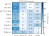 |
Fig. 4. Fraction of objects assigned to each type of ionization by the different explored diagnostic schemes for the full NMJ sample analyzed along this study. Colors, labels and legends are the same as in Fig. 3. |
By comparing the different methods, we could estimate the possible contamination between different types and possible missing sources. WHaD and WHaDoO are the methods that better recover AGNs. Thus, assuming that the fraction recovered by those methods is the closest to the real one, then the methods based on the BPT diagrams underestimate the fraction of AGNs by a factor between 1.5–3. The missing AGNs are distributed in the remaining groups, contaminating them. As the fraction of RGs recovered by all methods that include this type is essentially the same the missing AGNs are contaminating both the unknown+mixed group and the SFGs type. If we adopt 10% as the maximum fraction of unknown+mixed ionizing sources (based on the BPT-N2+WHa method), then it is fair to estimate that ∼23–25% of the objects classified as SFGs by the BPT-N2 and BPT-ALL diagrams most probably host an AGN. Following a similar reasoning, ∼3–5% of the SFGs based on the BPT-N2 and BPT-ALL schemes would be RGs (based on the other schemes). Those numbers may have an impact on the interpretation of galaxy properties (e.g., oxygen abundances) and patterns (e.g., SFMS), even though they are not particularly large (few percent), as we discuss later.
The diagrams using EW(Hα), apart from WHaD+O, are the ones with the lowest number of galaxies classified as mixed or unknown (< 9%) and a rather low number of SFGs, between ∼26–55%. This latter fraction is very similar to the one that result from the BPT diagrams, once considering the possible contamination described before. Thus, we conclude that they are the diagrams that provide the cleanest selection of SFGs (except the WHaO and WHaDaO diagrams). On the contrary, they show a non-negligible pollution in the AGN group, difficult to estimate, as they are also the diagrams that better select these targets. Being conservative, we could estimate this contamination in ∼25%, by assuming that all galaxies classified as unknown by the WHaO and WHaDoO diagrams (∼8%) are polluting the AGN group.
The WHaD+O method was introduced to minimize the cross-contamination. As a result, it is the method that provides the largest number of objects with a unknown ionization (∼34%), not being particularly good in maximizing the recovery of AGNs (∼6%) or SFGs (∼36%).
4. Discussion
In this study, we explored how galaxies whose ionization is dominated by different physical mechanisms are distributed along frequently used and new diagnostic diagrams to evaluate how we classify the ionization using them. In particular, we selected a set of archetypal galaxies associated with recent SF (LTGs), the absence of recent SF (ETGs), and a set of known AGNs selected using different methods independent of the explored classification schemes. The main result of our exploration is that the most frequently adopted procedures, based on the BPT diagrams, do not provide a robust classification of the ionization. They maximize the number of SFGs, polluting them with a significant number of AGNs and RG (∼30% of the objects), neglecting the RG group, and significantly underestimating the number of AGNs (∼30%) or missclassifying them. A relevant result of this analysis is that there is a region in the BPT diagrams where the three archetypal groups of ionizing sources overlap: at the right-bottom end of the classical location of H II regions, in the BPT-N2 diagram (where more metallic regions are found Espinosa-Ponce et al. 2022; Lugo-Aranda et al. 2024). This may sound counterintuitive, as we have learned that the line ratios reflect the physical conditions of the ionized gas (e.g., metallicity, density, spatial distribution), and the properties of the ionizing source (e.g., its strength and shape). However, this relation between line ratios and physical/ionizing source properties is not univocal, and it is affected by degeneracies. We are aware of and accustomed to these degeneracies in studies of other galaxy properties, such as their stellar populations. However, they are often bypassed in the exploration of ionization.
We have several examples of very different ionizing sources that could populate this area in the BPT-N2 diagram: (i) high-metallicity H II regions frequently found in early-spirals are found there (e.g., Sánchez et al. 2015; Espinosa-Ponce et al. 2020; Lugo-Aranda et al. 2024), as predicted by well-known photoionization models (e.g., K01, Morisset et al. 2016; ii) post-AGB ionization due to hot and low-mass evolved stars (e.g., Lacerda et al. 2018), also in agreement with photoionization models (e.g., Morisset et al. 2016; iii) shock-ionization due to low-scale and moderate-velocity and/or galactic-scale and high-velocity winds (e.g., López-Cobá et al. 2017, 2020), as predicted by shock models (e.g., Allen et al. 2008); and (iv) AGNs, in particular bona-fide X-ray-selected ones (e.g., Osorio-Clavijo et al. 2023). We should note that AGN photoionization models predict line ratios below both the K01 and K03 for low-metallicity AGNs (e.g., Groves et al. 2006). However, to our knowledge, there is no quantification of possible misclassifications and contamination from the different sources in the literature, like the one discussed here.
Our results indicate that there is no optimal selection criterion independent of the science case. For instance, if the main goal of an exploration is to extract all possible star-forming (or active galactic nuclei) irrespective of the possible contaminations, the use of the BPT-ALL (or the WHaDO) is recommended. If, for instance, the science goal is to trace the properties of a particular population (e.g, characterizing the mass-metallicity relation or the SFMS), minimizing the potential contamination by other selection processes, the WHaD+O scheme would be recommended. Otherwise, we may interpret as changes in the metallicity or the SFR what in reality is pollution by different ionizing processes (e.g., Vale Asari et al. 2019). In this sense, it is important to realize that the results and their interpretation would depend strongly on the adopted selection criteria. However, this is not a general conclusion either. It depends on the ionization type. We should stress that, based on our results, it is not recommended to use the classical BPT diagrams in any exploration involving RGs and AGNs.
4.1. How well we can select AGNs beyond the diagnostic diagram approach
The main results from this study regarding AGNs are related to the assumptions of the methods adopted to select our archetypal subsamples: X-AGNs, I-AGNs, O-AGNs, and R-AGNs. However, as in the case of diagnostic diagrams, many of the selection procedures designed using multiwavelength photometry are based on different assumptions and the actual knowledge and state-of-the-art at the moment when they were developed. This has a clear impact on the number of recovered AGNs and the discrepancies in their selection of these objects using each method (as summarized in Table 2). For instance, X-AGNs are considered the most reliable tracers of nuclear activity due to the hard X-ray emission from the hot corona around supermassive black holes, which is less affected by obscuration and orientation effects; however, X-ray surveys lack uniform sky coverage and/or completeness at faint flux levels (where the could be confused with X-ray binaries too). On the other hand, I-AGNs leverage the reprocessed emission from warm dust in the obscuring torus (e.g., Elitzur 2006), enabling the detection of both obscured and unobscured AGNs. Furthermore, the adopted IR dataset has an almost uniform coverage of the sky. The criteria adopted to select O-AGNs, based on the ultraviolet excess (UVX, Sandage 1965; Schmidt & Green 1983; Boyle et al. 1990), are effective for identifying just unobscured AGNs with blue colors in color–color space (e.g., Trammell et al. 2007; Richards et al. 2009), but suffer from significant biases against dusty or reddened sources (e.g., Benn et al. 1998) and host galaxy contamination that may be dominant in the NMJ sample. This explains why this is the AGN subsample with the lowest number of objects. Lastly, radio-selected AGNs (R-AGNs) represent a distinct population characterized by synchrotron emission from relativistic jets (Urry & Padovani 1995), typically found in massive elliptical galaxies and dense environments (e.g., Sánchez & González-Serrano 1999; Best 2000). Unlike the other groups, many R-AGNs show no optical AGN signatures and may be remnants of past activity, making them particularly challenging to classify using standard emission-line diagnostics, in particular to separate them from RGs.
Number and fraction of AGNs derived using different methods, and agreement between them.
It is beyond the scope of this study to revise the different procedures adopted in the literature to select AGNs considering of the current results. However, following our methodology, we explored how the different ionization types adopted in this study (SFGs, ETGs, and AGNs) are distributed in the space of parameters adopted to select the subsamples of AGNs described before. We adopted the WHaD+O scheme described above to segregate the galaxies in the NMJ catalog into the three different groups depending on the dominant ionization. This ensures the minimum cross-contamination from the different groups, at the expense of the lowest number of correctly classified galaxies. This is a good example of a case in which pollution should be avoided, as we are to explore the typical properties of the three different types, minimizing the contamination by other types.
Figure 5 shows the distribution of all galaxies and the different subsamples based on their dominant ionization in the diagrams adopted to select X-AGNs (HR vs. LX), I-AGNs (W1-W2 vs. W1), O-AGNs (NUV-u vs. u-g) and R-AGNs (Fint/Fpeak vs. Fint at 1.4 GHz). A visual exploration of this figure demonstrates that there are significant differences among the completeness of the different methods. Quantitatively, ∼83% of the AGNs selected by the WHaD+O scheme would be classified as X-AGNs (if X-ray data were available), in contrast, only 23% of them would be classified as I-AGNs, and just a 1–4% as O-AGNs and R-AGNs (if the proper data were available). The contamination from non-AGN ionization is also different for each selection criteria: (i) ∼20% for X-AGNs (∼4% being SFGs, and ∼17% being RGs); (ii) ∼1% for I-AGNs (mostly SFGs); (iii) < 0.2% for O-AGNs (mostly SFGs); and (iv) ∼11% for R-AGNs (mostly RGs). Thus, despite their different ability to select complete samples of AGNs, the contamination ratio is rather low.
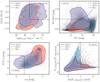 |
Fig. 5. Distribution of the full sample of galaxies in the four set of properties used to select the candidates to AGNs employed in this study: Top-left panel: X-ray properties, showing the X-ray hardness ratio as a function of the X-ray luminosity. Top-right panel: IR properties, showing the WISE W1 − W2 color as a function of the WISE W2 magnitude. Bottom-left panel: UV-optical properties, showing NUV − u color as a function of u − g one. Bottom-right panel: Radio properties, showing the ratio between the integrated and peak intensity at 1.4 GHz as a function of the integrated intensity. Each panel adopts the same symbols and color scheme: (i) solid circles correspond to the full sample of galaxies with measured properties, comprising 1390 objects for the X-ray panel, 541 478 for the IR one, 547 928 for the UV-optical one, and 15 839 for the radio one; (ii) contours represent the area that encircles 95% of the objects with ionization classified as star-forming (SFGs, blue), retired galaxies (RGs, red), and AGNs (purple) using out final classification scheme described in Sect. 3; (iii) dashed-lines show the demarcation lines described in Sect. 3 to select the AGN candidates using the represented properties. |
By far, the most effective method seems to be the X-ray selection, although it presents the highest contamination, followed by the selection based on IR photometry, as already shown in Table 2. Furthermore, it presents a rather low contamination rate by non AGNs. On the contrary, the less effective methods are those based on UV/optical colors and radio frequencies. These results are not surprising, as those later methods select two very particular sub-sets of AGNs: (i) unobscured AGNs in the first case, and (ii) radio-loud ones that are known to be just a ∼10% of the AGNs, when considered only the extended sources, as we did in our selection criteria (e.g., Urry & Padovani 1995; Rafter et al. 2009).
In the light of these results, and despite the problems described and discussed in this study, it seems that the selection of AGNs (and other sources of ionization) using the information provided by the emission lines in the optical regime remains a powerful and efficient method compared with others proposed in the literature. This is highlighted in Table 2, where we include the fraction of AGNs recovered using the WHaD+O method for the four subsamples discussed before (X-AGNs, I-AGNs, O-AGNs and R-AGNs), and the cross-matching between them. The fraction of AGNs recovered using optical emission lines is much higher than the one recovered using any of the other four different methods using multiwavelength observations. Indeed, there is only one AGN (candidate) that was selected using the four methods simultaneously in the entire NMJ sample. This target was also recovered using the WHaD+O method.
4.2. AGN selection and the properties of host galaxies
The (proper) selection of AGNs and a good separation of them from SFGs and RGs are relevant not only for their understanding, interesting per se, but also for studies of galaxy evolution. Nuclear activity has become extremely relevant in this context due to the three main results: (i) the discovery of strong correlations between black hole mass and host galaxy properties such as bulge luminosity, mass, and velocity dispersion (see reviews by Kormendy & Ho 2013; Graham 2016; ii) the need for an energetic mechanism (likely AGN feedback) to heat or expel gas in massive galaxies, thus quenching SF and reconciling the high-mass end of observed galaxy luminosity functions with theoretical predictions from semi-analytic models (e.g., Kauffmann & Haehnelt 2000; Bower et al. 2006; De Lucia & Blaizot 2007; Somerville et al. 2008) and cosmological simulations (e.g., Sijacki et al. 2015; Rosas-Guevara et al. 2016; Dubois et al. 2016); and (iii) the requirement for a rapid (≲1 Gyr) morphological transformation from star-forming spirals to quiescent ellipticals over the last 8 Gyr, based on population studies (e.g., Bell et al. 2004; Faber et al. 2007; Schiminovich et al. 2007).
Together, these results suggest that super-massive black holes co-evolve with galaxies, particularly their spheroidal components (e.g., Kormendy & Ho 2013), and that AGN feedback plays a critical role in galaxy evolution. Specifically, negative AGN feedback may heat or eject gas, quench SF, and drive morphological transitions between galaxy types (Silk & Rees 1998; Silk 2005; Hopkins et al. 2010), potentially explaining the evolutionary link between central and extended LI(N)ER proposed by Belfiore et al. (2017).
Observational support for this scenario includes the finding by K03 that type-II AGNs occupy the “green valley” in the color-magnitude diagram between the blue cloud of star-forming galaxies and the red sequence of quiescent ones. This has been confirmed at intermediate redshift for type-I AGNs as well (e.g., Sánchez et al. 2004), and reinforced by later studies (e.g., Schawinski et al. 2010; Torres-Papaqui et al. 2012, 2013; Ortega-Minakata 2015). AGN hosts also appear in transitional zones of other diagrams, such as the SFR versus stellar mass (e.g., Cano-Díaz et al. 2016; Sánchez et al. 2018, 2022; Lacerda et al. 2020). Furthermore, they seem to be located in early-type massive galaxies; thus, in a morphological transition phase between disk-dominated and bulge-dominated galaxies.
As suggested before, all these results rely on a proper selection of galaxies that host an AGN and a clear distinction between galaxies that are actively star-forming or have already ceased to form stars. It is beyond the scope of this study to explore in detail the properties of AGNs host galaxies and their connection with galaxy evolution. However, we should at least demonstrate that our proposed WHaD+O selection reproduces the main results described in the literature. To do so, we explore the distribution of our selected samples of SFGs, RGs, and AGNs extracted from the NMJ catalog using this selection criterion in three diagrams that illustrate the evolutionary stage of galaxies: (i) the sSFR-M* diagram, which highlights whether or not a galaxy is actively star-forming (e.g., Rodríguez-Puebla et al. 2020), (ii) the D4000-M*, illustrating the presence (or absence) of a young stellar population during a larger period than the one traced by recent SF (e.g., Blanton & Moustakas 2009); and (iii) the Re-M* diagram, that traces the compactness of a galaxy, tracing whether it is dominated by a disk or a bulge (e.g., Hashemizadeh et al. 2022).
The results of this exploration are shown in Fig. 6, illustrating that in general our proposed WHaD+O selection replicates previous results. In the sSFR-M* diagram the SFGs follow a clear trend, with higher (lower) sSFR at lower (higher) masses, expanding up to M* < 1010.5 M⊙. On the contrary RGs cover a range of M* that overlaps with SFGs above 109.5 M⊙, but covering a much lower regime of sSFRs, distributing themselves as a cloud rather than following a clear sequence. As expected from the literature, AGN hosts are located in the knee/transition regime between the other two galaxy groups, following somehow the same trend found for the SFGs, but at a mass regime covered by the RGs.
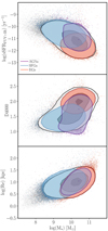 |
Fig. 6. Distribution of the full sample of galaxies along the sSFR-M* plane (top panel), D4000-M* plane (middle panel), and Re-M* plane (bottom panel). Symbols and contours have the same meaning as those described in the caption of Fig. 5. |
The D4000-M* shows similar results, with SFGs showing lower D4000 values than RGs, highlighting the presence of a young stellar population that is absent in this latter group. AGN hosts are clearly located in the transition phase between both groups, with M* covering the highest value end of SFGs and overlapping with those of RGs, while D4000 covers a wide range of values, representative of both young and old stellar populations. Thus, AGN hosts seem to be under transition between SFGs and RGs for a time larger than the usually assumed timescale of an active nucleus (e.g., Sánchez et al. 2018; Lacerda et al. 2020).
Finally, the Re-M* diagram shows the clear morphological distinction between SFGs, which are found at the expected location of disk-dominated galaxies, and RGs, which trace the location of bulge-dominated galaxies (e.g., Shen et al. 2003). To our knowledge, this diagram has not been explored in the context of AGN hosts; however, their distribution is not surprising, as they are located again between SFGs and RGs. They follow a relation with the same slope as the one traced by bulge-dominated galaxies, but slightly shifted toward lower M*.
5. Conclusions
We have evaluated how the diagnostic diagrams classify the dominant physical processes that ionize the ISM in galaxies. In summary, we found that:
-
Classification schemes that rely solely on the classical BPT diagrams systematically overestimate the number of star-forming galaxies, underestimate the number of AGNs, and cannot recognise RGs ionisation. Quantitatively, BPT-based selections miss ∼30% of bona fide AGNs and misclassify a similar fraction of RGs and AGNs as star-forming systems.
-
RGs can only be isolated robustly in the Hα equivalent width since traditional BPT boundaries leave them hidden among AGNs or composite objects.
-
Diagnostics that couple EW(Hα) to an additional observable (e.g., WHaN, WHaD, and the new WHaO diagram) provide a far cleaner separation of ionisation mechanisms. In particular, the combination of WHaD and WHaO recovers ≳60–90% of independently selected AGNs, while keeping SF contamination below ∼10%.
-
A final, balanced selection recipe that (i) identifies RGs with EW(Hα) < 3 Å and (ii) labels galaxies as SF or AGN only when both WHaD and WHaO concur, yields the lowest cross-contamination and reproduces the expected loci of SF, RG, and AGN hosts in sSFR-M⋆, D4000-M⋆, and Re-M⋆ diagrams.
-
Multiwavelength AGN samples (X-ray, IR, UV/optical, radio) occupy partly disjoint regions of optical diagnostic diagram; this diversity explains why any single optical criterion alone cannot catch all flavours of AGNs.
One final conclusion of this exploration is that we ought to re-evaluate carefully how we classify the ionization in galaxies and, in particular, we ought to critically revise the results presented in the literature using classical diagnostic diagrams and the varying ionization types derived from them.
Furthermore, following Sánchez et al. (2021, 2024), we will attempt to implement the current methodology to existing IFS datasets in a future study. We will aim to explore how the use of spatially resolved information would improve the classification of the ionizing sources in galaxies.
We prefer to label these two samples as LTGs and ETGs, instead of SFGs and RGs, as we reserve the last terms for the galaxies selected using the diagnostic diagram.
To our knowledge it has been used in very few occasions, and not focused on the study of different ionizing sources (e.g., Stasińska et al. 2015).
Acknowledgments
We thanks the anonymous referee for the comments that have improved this manuscript. SFS thanks the support by UNAM PASPA – DGAPA and the SECIHTI CBF-2025-I-236 project. Authors acknowledge financial support from the Spanish Ministry of Science and Innovation (MICINN), project PID2022-136598NB-C31 (ESTALLIDOS). JSA acknowledges support from the EU UNDARK project (A way of making Europe: project number 101159929). EP acknowledges support from the Spanish MICINN funding grant PGC2018-101931-B-I00 and Severo Ochoa grant CEX2021-001131-S funded by MCIN/AEI/10.13039/501100011033. OGM thanks the support by DGAPA-PAPIIT IN109123 and SECIHTI CF2023-G100 projects. We thank the creators of the NSA, MPA-JHU and SDSS surveys. The NASA-Sloan Atlas was created by Michael Blanton, with extensive help and testing from Eyal Kazin, Guangtun Zhu, Adrian Price-Whelan, John Moustakas, Demitri Muna, Renbin Yan and Benjamin Weaver. Renbin Yan provided the detailed spectroscopic measurements for each SDSS spectrum. David Schiminovich kindle provided the input GALEX images. We thank also Nikhil Padmanabhan, David Hogg, Doug Finkbeiner and David Schlegel for their work on SDSS image infrastructure. The MPA-JHU catalog was collected by a team made up of Stephane Charlot, Guinevere Kauffmann and Simon White (MPA), Tim Heckman (JHU), Christy Tremonti (University of Arizona – formerly JHU) and Jarle Brinchmann (Centro de Astrofísica da Universidade do Porto – formerly MPA). SDSS-III is managed by the Astrophysical Research Consortium for the Participating Institutions of the SDSS-III Collaboration including the University of Arizona, the Brazilian Participation Group, Brookhaven National Laboratory, University of Cambridge, University of Florida, the French Participation Group, the German Participation Group, the Instituto de Astrofisica de Canarias, the Michigan State/Notre Dame/JINA Participation Group, Johns Hopkins University, Lawrence Berkeley National Laboratory, Max Planck Institute for Astrophysics, New Mexico State University, New York University, Ohio State University, Pennsylvania State University, University of Portsmouth, Princeton University, the Spanish Participation Group, University of Tokyo, University of Utah, Vanderbilt University, University of Virginia, University of Washington, and Yale University. This research has made use of data obtained from the 4XMM XMM-Newton serendipitous stacked source catalogue 4XMM-DR14s compiled by the institutes of the XMM-Newton Survey Science center selected by ESA. This work is based on data from the Faint Images of the Radio Sky at Twenty Centimeters (FIRST) survey, obtained from the December 2014 data release (first_14dec17.fits.gz), available at https://third.ucllnl.org/cgi-bin/firstcutout.
References
- Agostino, C. J., & Salim, S. 2019, ApJ, 876, 12 [NASA ADS] [CrossRef] [Google Scholar]
- Aihara, H., Allende Prieto, C., An, D., et al. 2011, ApJS, 193, 29 [NASA ADS] [CrossRef] [Google Scholar]
- Allen, M. G., Groves, B. A., Dopita, M. A., Sutherland, R. S., & Kewley, L. J. 2008, ApJS, 178, 20 [Google Scholar]
- Assef, R. J., Stern, D., Noirot, G., et al. 2018, ApJS, 234, 23 [Google Scholar]
- Baldwin, J. A., Phillips, M. M., & Terlevich, R. 1981, PASP, 93, 5 [Google Scholar]
- Becker, R. H., White, R. L., & Helfand, D. J. 1995, ApJ, 450, 559 [Google Scholar]
- Belfiore, F., Maiolino, R., Maraston, C., et al. 2017, MNRAS, 466, 2570 [Google Scholar]
- Belfiore, F., Santoro, F., Groves, B., et al. 2022, A&A, 659, A26 [NASA ADS] [CrossRef] [EDP Sciences] [Google Scholar]
- Bell, E. F., McIntosh, D. H., Barden, M., et al. 2004, ApJ, 600, L11 [NASA ADS] [CrossRef] [Google Scholar]
- Benn, C. R., Vigotti, M., Carballo, R., Gonzalez-Serrano, J. I., & Sanchez, S. F. 1998, MNRAS, 295, 451 [NASA ADS] [CrossRef] [Google Scholar]
- Best, P. N. 2000, MNRAS, 317, 720 [NASA ADS] [CrossRef] [Google Scholar]
- Binette, L., Magris, C. G., Stasińska, G., & Bruzual, A. G. 1994, A&A, 292, 13 [NASA ADS] [Google Scholar]
- Blanton, M. R., & Moustakas, J. 2009, ARA&A, 47, 159 [Google Scholar]
- Blanton, M. R., Kazin, E., Muna, D., Weaver, B. A., & Price-Whelan, A. 2011, AJ, 142, 31 [NASA ADS] [CrossRef] [Google Scholar]
- Bower, R. G., Benson, A. J., Malbon, R., et al. 2006, MNRAS, 370, 645 [Google Scholar]
- Boyle, B. J., Fong, R., Shanks, T., & Peterson, B. A. 1990, MNRAS, 243, 1 [NASA ADS] [Google Scholar]
- Brightman, M., & Nandra, K. 2011, MNRAS, 413, 1206 [NASA ADS] [CrossRef] [Google Scholar]
- Brinchmann, J., Charlot, S., White, S. D. M., et al. 2004, MNRAS, 351, 1151 [Google Scholar]
- Cano-Díaz, M., Sánchez, S. F., Zibetti, S., et al. 2016, ApJ, 821, L26 [Google Scholar]
- Catalán-Torrecilla, C., Gil de Paz, A., Castillo-Morales, A., et al. 2015, A&A, 584, A87 [NASA ADS] [CrossRef] [EDP Sciences] [Google Scholar]
- Cid Fernandes, R., Stasińska, G., Schlickmann, M. S., et al. 2010, MNRAS, 403, 1036 [Google Scholar]
- Cid Fernandes, R., Stasińska, G., Mateus, A., & Vale Asari, N. 2011, MNRAS, 413, 1687 [Google Scholar]
- Cid Fernandes, R., Carvalho, M. S., Sánchez, S. F., de Amorim, A., & Ruschel-Dutra, D. 2021, MNRAS, 502, 1386 [NASA ADS] [CrossRef] [Google Scholar]
- Cluver, M. E., Jarrett, T. H., Dale, D. A., et al. 2017, ApJ, 850, 68 [Google Scholar]
- Comerford, J. M., Negus, J., Müller-Sánchez, F., et al. 2020, ApJ, 901, 159 [NASA ADS] [CrossRef] [Google Scholar]
- De Lucia, G., & Blaizot, J. 2007, MNRAS, 375, 2 [Google Scholar]
- Donley, J. L., Koekemoer, A. M., Brusa, M., et al. 2012, ApJ, 748, 142 [Google Scholar]
- Dopita, M. A., Koratkar, A. P., Evans, I. N., et al. 1996, ASP Conf. Ser., 103, 44 [Google Scholar]
- Dors, O. L., Jr., Krabbe, A., Hägele, G. F., & Pérez-Montero, E. 2011, MNRAS, 415, 3616 [NASA ADS] [CrossRef] [Google Scholar]
- Dubois, Y., Peirani, S., Pichon, C., et al. 2016, MNRAS, 463, 3948 [Google Scholar]
- Elitzur, M. 2006, New Astron. Rev., 50, 728 [CrossRef] [Google Scholar]
- Espinosa-Ponce, C., Sánchez, S. F., Morisset, C., et al. 2020, MNRAS, 494, 1622 [Google Scholar]
- Espinosa-Ponce, C., Sánchez, S. F., Morisset, C., et al. 2022, MNRAS, 512, 3436 [NASA ADS] [CrossRef] [Google Scholar]
- Faber, S. M., Willmer, C. N. A., Wolf, C., et al. 2007, ApJ, 665, 265 [Google Scholar]
- Flores-Fajardo, N., Morisset, C., Stasińska, G., & Binette, L. 2011, MNRAS, 415, 2182 [Google Scholar]
- González Delgado, R. M., Cid Fernandes, R., Pérez, E., et al. 2016, A&A, 590, A44 [NASA ADS] [CrossRef] [EDP Sciences] [Google Scholar]
- Graham, A. W. 2016, Gal. Bulges, 418, 263 [Google Scholar]
- Groves, B. A., Heckman, T. M., & Kauffmann, G. 2006, MNRAS, 371, 1559 [NASA ADS] [CrossRef] [Google Scholar]
- Hashemizadeh, A., Driver, S. P., Davies, L. J. M., et al. 2022, MNRAS, 515, 1175 [NASA ADS] [CrossRef] [Google Scholar]
- Heckman, T. M. 1987, in Observational Evidence of Activity in Galaxies, eds. E. E. Khachikian, & K. J. Fricke, 121, 421 [Google Scholar]
- Hopkins, P. F., Bundy, K., Croton, D., et al. 2010, ApJ, 715, 202 [Google Scholar]
- Ivezić, Ž., Menou, K., Knapp, G. R., et al. 2002, AJ, 124, 2364 [CrossRef] [Google Scholar]
- Jarrett, T. H., Cohen, M., Masci, F., et al. 2011, ApJ, 735, 112 [Google Scholar]
- Jaskot, A. E., & Oey, M. S. 2013, ApJ, 766, 91 [Google Scholar]
- Kauffmann, G., & Haehnelt, M. 2000, MNRAS, 311, 576 [Google Scholar]
- Kauffmann, G., Heckman, T. M., Tremonti, C., et al. 2003, MNRAS, 346, 1055 [Google Scholar]
- Kehrig, C., Monreal-Ibero, A., Papaderos, P., et al. 2012, A&A, 540, A11 [Google Scholar]
- Kennicutt, R. C., Jr. 1983, ApJ, 272, 54 [NASA ADS] [CrossRef] [Google Scholar]
- Kewley, L. J., Dopita, M. A., Sutherland, R. S., Heisler, C. A., & Trevena, J. 2001, ApJ, 556, 121 [Google Scholar]
- Kewley, L. J., Groves, B., Kauffmann, G., & Heckman, T. 2006, MNRAS, 372, 961 [Google Scholar]
- Kewley, L. J., Maier, C., Yabe, K., et al. 2013, ApJ, 774, L10 [Google Scholar]
- Kewley, L. J., Nicholls, D. C., & Sutherland, R. S. 2019, ARA&A, 57, 511 [Google Scholar]
- Kimball, A. E., Ivezić, Ž., Wiita, P. J., & Schneider, D. P. 2011, AJ, 141, 182 [NASA ADS] [CrossRef] [Google Scholar]
- Kormendy, J., & Ho, L. C. 2013, ARA&A, 51, 511 [Google Scholar]
- Lacerda, E. A. D., Cid Fernandes, R., Couto, G. S., et al. 2018, MNRAS, 474, 3727 [Google Scholar]
- Lacerda, E. A. D., Sánchez, S. F., Cid Fernandes, R., et al. 2020, MNRAS, 492, 3073 [Google Scholar]
- Lange, R., Driver, S. P., Robotham, A. S. G., et al. 2015, MNRAS, 447, 2603 [CrossRef] [Google Scholar]
- Levi, M., Allen, L. E., Raichoor, A., et al. 2019, Bull. Am. Astron. Soc., 51, 57 [Google Scholar]
- López-Cobá, C., Sánchez, S. F., Cruz-González, I., et al. 2017, ApJ, 850, L17 [CrossRef] [Google Scholar]
- López-Cobá, C., Sánchez, S. F., Bland-Hawthorn, J., et al. 2019, MNRAS, 482, 4032 [Google Scholar]
- López-Cobá, C., Sánchez, S. F., Anderson, J. P., et al. 2020, AJ, 159, 167 [Google Scholar]
- Lugo-Aranda, A. Z., Sánchez, S. F., Barrera-Ballesteros, J. K., et al. 2024, MNRAS, 528, 6099 [NASA ADS] [CrossRef] [Google Scholar]
- Martin, C., Barlow, T., Barnhart, W., et al. 2003, SPIE Conf. Ser., 4854, 336 [NASA ADS] [Google Scholar]
- Melnyk, O., Plionis, M., Elyiv, A., et al. 2013, A&A, 557, A81 [NASA ADS] [CrossRef] [EDP Sciences] [Google Scholar]
- Morisset, C., Delgado-Inglada, G., Sánchez, S. F., et al. 2016, A&A, 594, A37 [NASA ADS] [CrossRef] [EDP Sciences] [Google Scholar]
- Muñoz Santos, D., Pappalardo, C., Miranda, H., et al. 2025, A&A, 701, A271 [NASA ADS] [CrossRef] [EDP Sciences] [Google Scholar]
- Ortega-Minakata, R. A. 2015, Ph.D. Thesis, Universidad de Guanajuato [Google Scholar]
- Osorio-Clavijo, N., Gonzalez-Martín, O., Sánchez, S. F., Guainazzi, M., & Cruz-González, I. 2023, MNRAS, 522, 5788 [NASA ADS] [CrossRef] [Google Scholar]
- Osterbrock, D. E. 1989, Astrophysics of Gaseous Nebulae and Active Galactic Nuclei (University Science Books) [Google Scholar]
- Osterbrock, D. E., Tran, H. D., & Veilleux, S. 1992, ApJ, 389, 305 [Google Scholar]
- Overzier, R. A., Heckman, T. M., Tremonti, C., et al. 2009, ApJ, 706, 203 [NASA ADS] [CrossRef] [Google Scholar]
- Rafter, S. E., Crenshaw, D. M., & Wiita, P. J. 2009, AJ, 137, 42 [Google Scholar]
- Renzini, A., & Peng, Y.-J. 2015, ApJ, 801, L29 [Google Scholar]
- Richards, G. T., Myers, A. D., Gray, A. G., et al. 2009, ApJS, 180, 67 [Google Scholar]
- Rodríguez-Puebla, A., Avila-Reese, V., Cano-Díaz, M., et al. 2020, ApJ, 905, 171 [Google Scholar]
- Rosas-Guevara, Y., Bower, R. G., Schaye, J., et al. 2016, MNRAS, 462, 190 [CrossRef] [Google Scholar]
- Roy, N., Bundy, K., Cheung, E., et al. 2018, ApJ, 869, 117 [NASA ADS] [CrossRef] [Google Scholar]
- Sánchez, S. F. 2020, ARA&A, 58, 99 [Google Scholar]
- Sánchez, S. F., & González-Serrano, J. I. 1999, A&A, 352, 383 [Google Scholar]
- Sánchez, S. F., Jahnke, K., Wisotzki, L., et al. 2004, ApJ, 614, 586 [CrossRef] [Google Scholar]
- Sánchez, S. F., Rosales-Ortega, F. F., Iglesias-Páramo, J., et al. 2014, A&A, 563, A49 [CrossRef] [EDP Sciences] [Google Scholar]
- Sánchez, S. F., Pérez, E., Rosales-Ortega, F. F., et al. 2015, A&A, 574, A47 [NASA ADS] [CrossRef] [EDP Sciences] [Google Scholar]
- Sánchez, S. F., Avila-Reese, V., Hernandez-Toledo, H., et al. 2018, Rev. Mex. Astron. Astrofis., 54, 217 [Google Scholar]
- Sánchez, S. F., Avila-Reese, V., Rodríguez-Puebla, A., et al. 2019, MNRAS, 482, 1557 [Google Scholar]
- Sánchez, S. F., Walcher, C. J., Lopez-Cobá, C., et al. 2021, Rev. Mex. Astron. Astrofis., 57, 3 [Google Scholar]
- Sánchez, S. F., Barrera-Ballesteros, J. K., Lacerda, E., et al. 2022, ApJS, 262, 36 [CrossRef] [Google Scholar]
- Sánchez, S. F., Lugo-Aranda, A. Z., Sánchez Almeida, J., et al. 2024, A&A, 682, A71 [NASA ADS] [CrossRef] [EDP Sciences] [Google Scholar]
- Sandage, A. 1965, ApJ, 141, 1560 [NASA ADS] [CrossRef] [Google Scholar]
- Schawinski, K., Urry, C. M., Virani, S., et al. 2010, ApJ, 711, 284 [NASA ADS] [CrossRef] [Google Scholar]
- Schiminovich, D., Wyder, T. K., Martin, D. C., et al. 2007, ApJS, 173, 315 [Google Scholar]
- Schmidt, M., & Green, R. F. 1983, ApJ, 269, 352 [NASA ADS] [CrossRef] [Google Scholar]
- Shen, S., Mo, H. J., White, S. D. M., et al. 2003, MNRAS, 343, 978 [NASA ADS] [CrossRef] [Google Scholar]
- Sijacki, D., Vogelsberger, M., Genel, S., et al. 2015, MNRAS, 452, 575 [NASA ADS] [CrossRef] [Google Scholar]
- Silk, J. 2005, MNRAS, 364, 1337 [NASA ADS] [CrossRef] [Google Scholar]
- Silk, J., & Rees, M. J. 1998, A&A, 331, L1 [NASA ADS] [Google Scholar]
- Singh, R., van de Ven, G., Jahnke, K., et al. 2013, A&A, 558, A43 [NASA ADS] [CrossRef] [EDP Sciences] [Google Scholar]
- Somerville, R. S., Hopkins, P. F., Cox, T. J., Robertson, B. E., & Hernquist, L. 2008, MNRAS, 391, 481 [NASA ADS] [CrossRef] [Google Scholar]
- Stasińska, G., Vale Asari, N., Cid Fernandes, R., et al. 2008, MNRAS, 391, L29 [NASA ADS] [Google Scholar]
- Stasińska, G., Izotov, Y., Morisset, C., & Guseva, N. 2015, A&A, 576, A83 [NASA ADS] [CrossRef] [EDP Sciences] [Google Scholar]
- Strömgren, B. 1939, ApJ, 89, 526 [CrossRef] [Google Scholar]
- Teimoorinia, H., & Keown, J. 2018, MNRAS, 478, 3177 [Google Scholar]
- Torres-Papaqui, J. P., Coziol, R., Andernach, H., et al. 2012, Rev. Mex. Astron. Astrofis., 48, 275 [Google Scholar]
- Torres-Papaqui, J. P., Coziol, R., Plauchu-Frayn, I., Andernach, H., & Ortega-Minakata, R. A. 2013, Rev. Mex. Astron. Astrofis., 49, 311 [Google Scholar]
- Trammell, G. B., Vanden Berk, D. E., Schneider, D. P., et al. 2007, AJ, 133, 1780 [Google Scholar]
- Traulsen, I., Schwope, A. D., Lamer, G., et al. 2020, A&A, 641, A137 [NASA ADS] [CrossRef] [EDP Sciences] [Google Scholar]
- Tremonti, C. A., Heckman, T. M., Kauffmann, G., et al. 2004, ApJ, 613, 898 [Google Scholar]
- Urry, C. M., & Padovani, P. 1995, PASP, 107, 803 [NASA ADS] [CrossRef] [Google Scholar]
- Vale Asari, N., Couto, G. S., Cid Fernandes, R., et al. 2019, MNRAS, 489, 4721 [NASA ADS] [CrossRef] [Google Scholar]
- van der Wel, A., Franx, M., van Dokkum, P. G., et al. 2014, ApJ, 788, 28 [Google Scholar]
- Veilleux, S., & Osterbrock, D. E. 1987, ApJS, 63, 295 [Google Scholar]
- Veilleux, S., Shopbell, P. L., & Miller, S. T. 2001, AJ, 121, 198 [NASA ADS] [CrossRef] [Google Scholar]
- Veilleux, S., Cecil, G., & Bland-Hawthorn, J. 2005, ARA&A, 43, 769 [NASA ADS] [CrossRef] [Google Scholar]
- Wadadekar, Y. 2004, A&A, 416, 35 [NASA ADS] [CrossRef] [EDP Sciences] [Google Scholar]
- Wake, D. A., Bundy, K., Diamond-Stanic, A. M., et al. 2017, AJ, 154, 86 [Google Scholar]
- Wright, E. L., Eisenhardt, P. R. M., Mainzer, A. K., et al. 2010, AJ, 140, 1868 [Google Scholar]
- York, D. G., Adelman, J., Anderson, J. E., Jr., et al. 2000, AJ, 120, 1579 [NASA ADS] [CrossRef] [Google Scholar]
Appendix A: Diagnostic diagrams for different AGN selections
We present in this appendix the same diagnostic diagrams shown in Fig. 2, which compares the distribution of X-AGNs with that of the full sample of galaxies (NMJ) and both subsamples of LTGs and ETGs that are archetypal of star-forming and retired galaxies, corresponding to the other three samples of AGNs explored along this study: (i) I-AGNs (Fig. A.1, (ii) O-AGNs (Fig. A.2) and (iii) R-AGNs (Fig. A.3)
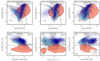 |
Fig. A.1. Same as Fig. 2, but showing the distribution of the IR-selected AGNs (I-AGNs) in the different panels as solid dark blue circles. |
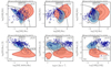 |
Fig. A.2. Same as Fig. 2, but showing the distribution of the optically selected AGNs (O-AGNs) in the different panels as solid dark blue squares. |
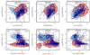 |
Fig. A.3. Same as Fig. 2, but showing the distribution of the radio-selected AGNs (R-AGNs) in the different panels as solid dark blue diamonds. |
All Tables
Number and fraction of AGNs derived using different methods, and agreement between them.
All Figures
|
Fig. 1. Comparison between the SFR provided by the MPA-JHU catalog and the one derived combining the IR and UV photometry as described in the text. The black dots correspond to each galaxy in the NMJ sample (i.e., the full sample of galaxies analyzed in this article) and each successive grey contour represents the area encircling a 90%, 65%, and a 15% of these points. The dashed-line represent the one-to-one relation. |
| In the text | |
|
Fig. 2. Distribution of the subsamples of galaxies across different diagnostic diagram. Top panels: Classical BPT diagrams (Baldwin et al. 1981), showing the distribution of O III/Hβ line ratio as a function of N II/Hα ratio (left panel), S II/Hα (middle panel), and O I/Hα (right panel). Solid and dot-dashed lines correspond to the demarcation lines proposed by K03 and K01 to distinguish between the different ionizing sources. Bottom panels: Diagrams comparing the distribution of Equivalent-width of Hα (WHα) as a function of (i) the N II/Hα ratio (left panel) WHaN diagram (Cid Fernandes et al. 2010; ii) the Hα velocity dispersion (σHα, middle panel), WHaD diagram (Sánchez et al. 2024); and (iii) the O III/O II line ratio (right panel), proposed here as the WHaO diagram. In each panel, the black dots correspond to the full NMJ sample and each successive grey contour represents the area encircling the 90%, 65%, and a 15% of these points. The blue (red) contour represent the area that encircles 90% of the values corresponding to the LT (ET) subsamples of galaxies, as defined in the text. Finally, the location of the X-ray-selected AGNs are shown as dark-blue stars. The D parameter derived for a set of 2D KS-tests comparing the distributions of the different subsamples are included on top of each panel, using the nomenclature L/E when comparing LTGs versus ETGs, E/A for ETGs versus X-AGNs, and L/A for LTGs versus X-AGNs. |
| In the text | |
|
Fig. 3. Differences found in the classification of the dominant ionization when using different diagnostics. Each panel comprises a heat-map showing the fraction of objects (color scale and values within each cell) assigned to each type of ionization by a different diagnostic diagram for a different subsample of galaxies (from the top left to bottom right): LTGs, ETGs, X-ray-selected AGNs (X-AGNs), IR-selected AGNs (I-AGNs), UV-optically selected AGNs (O-AGNs), and radio-selected AGNs (R-AGNs). Each heat-map column corresponds to the different ionizing types considered in this work, namely: (i) ionization associated with recent SFGs; (ii) mixed or unknown ionization (Mix/Unk); (iii) ionization usually found in non-star-forming and retired galaxies (RGs), due to hot evolved stars (Binette et al. 1994; Flores-Fajardo et al. 2011), and/or low-velocity shocks (Dopita et al. 1996); and (iv) ionization associated with AGNs and or shocks associated with galactic scale winds (e.g., López-Cobá et al. 2020). On the other hand, each row corresponds to a different diagnostic scheme, including the use of: (i) the classical diagram by Baldwin et al. (1981) that uses O III/Hβ and N II/Hα line ratios (BPT-N2); (ii) the three diagrams by Baldwin et al. (1981) that use the O III/Hβ vs. N II/Hα S II/Hα and O I/Ha line ratios (BPT-all); (iii) the BPT-N2 diagram including a cut in the equivalent width of Hα (BPT-N2+WHa), as described in Sánchez (2020); (iv) the WHaN diagram that uses the N II/Hα and the equivalent width of Hα (WHaN); (v) the diagram introduced by Sánchez et al. (2024) that uses N II/Hα and the velocity dispersion of Hα (WHaD); (vi) the new proposed diagram that uses O III/O II and the equivalent width of Hα (WHaO). Finally, we have three different combinations that use the WHaD and WHaO diagrams: (vii) WHaDoO, (viii) WHaDoO, and (ix) WHaD+O, as described in the text. |
| In the text | |
|
Fig. 4. Fraction of objects assigned to each type of ionization by the different explored diagnostic schemes for the full NMJ sample analyzed along this study. Colors, labels and legends are the same as in Fig. 3. |
| In the text | |
|
Fig. 5. Distribution of the full sample of galaxies in the four set of properties used to select the candidates to AGNs employed in this study: Top-left panel: X-ray properties, showing the X-ray hardness ratio as a function of the X-ray luminosity. Top-right panel: IR properties, showing the WISE W1 − W2 color as a function of the WISE W2 magnitude. Bottom-left panel: UV-optical properties, showing NUV − u color as a function of u − g one. Bottom-right panel: Radio properties, showing the ratio between the integrated and peak intensity at 1.4 GHz as a function of the integrated intensity. Each panel adopts the same symbols and color scheme: (i) solid circles correspond to the full sample of galaxies with measured properties, comprising 1390 objects for the X-ray panel, 541 478 for the IR one, 547 928 for the UV-optical one, and 15 839 for the radio one; (ii) contours represent the area that encircles 95% of the objects with ionization classified as star-forming (SFGs, blue), retired galaxies (RGs, red), and AGNs (purple) using out final classification scheme described in Sect. 3; (iii) dashed-lines show the demarcation lines described in Sect. 3 to select the AGN candidates using the represented properties. |
| In the text | |
|
Fig. 6. Distribution of the full sample of galaxies along the sSFR-M* plane (top panel), D4000-M* plane (middle panel), and Re-M* plane (bottom panel). Symbols and contours have the same meaning as those described in the caption of Fig. 5. |
| In the text | |
|
Fig. A.1. Same as Fig. 2, but showing the distribution of the IR-selected AGNs (I-AGNs) in the different panels as solid dark blue circles. |
| In the text | |
|
Fig. A.2. Same as Fig. 2, but showing the distribution of the optically selected AGNs (O-AGNs) in the different panels as solid dark blue squares. |
| In the text | |
|
Fig. A.3. Same as Fig. 2, but showing the distribution of the radio-selected AGNs (R-AGNs) in the different panels as solid dark blue diamonds. |
| In the text | |
Current usage metrics show cumulative count of Article Views (full-text article views including HTML views, PDF and ePub downloads, according to the available data) and Abstracts Views on Vision4Press platform.
Data correspond to usage on the plateform after 2015. The current usage metrics is available 48-96 hours after online publication and is updated daily on week days.
Initial download of the metrics may take a while.