| Issue |
A&A
Volume 704, December 2025
|
|
|---|---|---|
| Article Number | A8 | |
| Number of page(s) | 19 | |
| Section | Stellar structure and evolution | |
| DOI | https://doi.org/10.1051/0004-6361/202556888 | |
| Published online | 26 November 2025 | |
Surface activity of a Rossby sequence of cool Hyades stars⋆
1
Leibniz-Institute for Astrophysics Potsdam (AIP), An der Sternwarte 16, D-14482 Potsdam, Germany
2
Institute for Physics and Astronomy, University of Potsdam, D-14476 Potsdam, Germany
⋆⋆ Corresponding author: This email address is being protected from spambots. You need JavaScript enabled to view it.
Received:
17
August
2025
Accepted:
22
October
2025
Abstract
Aims. The Hyades cluster is key for the study of the rotational, activity, and chemical evolution of solar-like low-mass stars. We present quantitative surface-activity information for a sequence of 21 Hyades dwarf stars with effective temperatures 6160–3780 K (all cooler than the red edge of the Li dip), rotation periods 5–16 d, and normalized Rossby numbers (Ron) between 0.14 to 0.54 with respect to the Sun (Ro(Sun) = 1).
Methods. High-resolution Stokes-V spectra and a least-squares deconvolution of thousands of spectral lines per spectrum were employed to measure the longitudinal surface magnetic field. We obtained the velocities, lithium abundances, metallicity, and chromospheric Ca II infrared-triplet (IRT) fluxes from Stokes-I spectra.
Results. The average metallicity, +0.186 ± 0.045 (rms), for our stars with Teff ≥ 4200 K agrees well with the metallicity in the recent literature. The lithium abundances A(Li) range from 95-times solar (A(Li) ≈ + 3.0) on the warm end of the sample to 1/25 solar (A(Li) ≈ − 0.4) on the cool end. We confirm the tight relation of A(Li) with Teff and extend it to K–M stars with even lower Li abundances than previously measurable. A formal relation with rotational period and velocity in the sense of a higher Li abundance for faster rotators is present. Targets that rotate faster than v sin i of 6 km s−1 (Prot ≈ 8 d) appear to be Li saturated at A(Li) ≈3.0 dex. The Ca II IRT fluxes for our sample indicate (logarithmic) chromospheric radiative losses R′IRT in the range −4.0 to −4.9 in units of the bolometric flux. These radiative losses are also related to Teff, Prot, and v sin i, but opposite to A(Li), in an inverse sense with higher radiative losses for the slower, that is, cooler rotators. Longitudinal magnetic field strengths were measured in the range zero to −100 G and +150 G with phase-averaged disk-integrated unsigned values ⟨|B|⟩ of 15.4 ± 3.6(rms) G for targets warmer than ≈5000 K and 91 ± 61(rms) G for targets cooler than this. These unsigned field strengths are related to Prot, v sin i, and Ron, but in a dual-slope fashion. The short-period bona fide single M-target RSP 348 was found to be a double-lined spectroscopic binary with a classification dM3e+dM5e.
Conclusions. We conclude that the dependence on Rossby number of the surface activity tracers A(Li), R′IRT, and ⟨|B|⟩ on our Hyades dwarf sequence primarily originates from convective motions, expressed by its turnover time, and only to a smaller and sometimes inverse extent from surface rotation and its related additional mixing.
Key words: stars: activity / stars: magnetic field / stars: rotation / starspots / open clusters and associations: individual: Hyades
Based on data acquired with the Potsdam Echelle Polarimetric and Spectroscopic Instrument (PEPSI) using the Large Binocular Telescope (LBT). The LBT is an international collaboration among institutions in the United States, Italy, and Germany.
© The Authors 2025
 Open Access article, published by EDP Sciences, under the terms of the Creative Commons Attribution License (https://creativecommons.org/licenses/by/4.0), which permits unrestricted use, distribution, and reproduction in any medium, provided the original work is properly cited.
This article is published in open access under the Subscribe to Open model. This email address is being protected from spambots. You need JavaScript enabled to view it. to support open access publication.
1. Introduction
Stellar angular momentum loss and its associated spin-down due to magnetic braking are of key interest for understanding the evolution of our Sun in detail and our Solar System in general. Stars in open clusters always played an important role in determining the relation of rotation and age simply because their ensemble age can be determined, but also because of their homogeneous formation history, which is expressed, for example, by their unified metallicities. The stellar rotation period as a function of mass and age is the observable global parameter for a quantitative spin-down description (Kraft 1967; Skumanich 1972; Noyes et al. 1984, and many thereafter). This enabled the formulation of gyrochronology (Barnes 2007), the determination of the stellar age from a rotation period, with a (re)emphasis of stellar evolution and in particular of convective turnover timescales (Barnes & Kim 2010; Corsaro et al. 2021). For a complete spin-down picture, however, it became obvious that the surface magnetic field morphology plays a more dominant role (e.g., Mestel 1968; Garraffo et al. 2018) because the open field alone can funnel charged particles off the star and generate mass and angular-momentum loss, while the closed field only traps these particles, but does not add to the wind (Parker 1958, but see also Mestel 1968; Vidotto et al. 2014; van Saders et al. 2016; Jardine et al. 2017). Observational evidence for a magnetic morphology shift in older solar-type stars was presented from spectropolarimetry of bright field stars (e.g., Metcalfe et al. 2022, 2024). Questions related to the magnetic field such as how this field is anchored to the convection zone or the role of the small-scale field and its hemispheric current helicity remain largely unanswered (see, e.g., Hale 1927; Fan 2009; Rüdiger & Küker 2016).
Measurements of the surface magnetic fields of cool cluster stars are difficult to obtain because of the large distances of cluster stars compared to nearby field stars. They are therefore still rare (Folsom et al. 2018; Wanderley et al. 2024). The difficulty lies in the intrinsically weak Zeeman signals and in the spatially unresolvable coexistence of local bipolarity. The latter ensures that the longitudinal component of a surface magnetic field, when averaged over the visible hemisphere of a star, approaches near zero when the contributions from positive-polarity regions match those from negative polarity. A time series of spectra is required to break this symmetry. The polarization degree due to the Zeeman-effect from the kilo-Gauss magnetic field of sunspots is typically about 10%, and only 0.01% for electron-scattering processes (e.g., Solanki 1993). A signal from photospheric solar-like stellar magnetic fields is therefore best detected from circular polarization (CP), but requires high-resolution spectra with a high signal-to-noise ratio (S/N) over a wide wavelength range. The target brightness is thus a basic selection criterion. Only with the advent of spectrum-denoising methods (Donati et al. 1997; Carroll et al. 2007; Martinez González et al. 2008; Kochukhov et al. 2010; Tkachenko et al. 2013) was it possible to measure Gauss-level magnetic field strengths on solar-like cool stars as well, however, as compared to the many kiloGauss-strong fields of Ap stars. Folsom et al. (2018) were the first to apply even Zeeman-Doppler imaging (ZDI; Semel Semel 1989) to cluster stars, in particular, also to the Hyades and younger stellar associations. Two of the five Hyades targets observed by Folsom et al. (2018) were binaries (Mel25-151 and Mel25-43), and one was a possible binary (Mel25-179). The two remaining stars, RSP 68 and RSP 198, were confirmed single stars based on the absence of radial velocity (RV) variations. These two stars are also in the sample of the present paper.
One current working assumption is that only the open large-scale field in its lowest energy state contributes to the mass and angular momentum loss (Jardine et al. 2013). If this is so, a statistical relation should exist between magnetic field morphology and rotation period in the sense of slower rotation in the case of more open field lines. See et al. (2018)) used a sample of 22 solar-mass field stars from the literature that had a magnetic surface map and used them to determine the amount of open flux. The age span of their field-star sample was between 24 Myr and 5 Gyr, but with very uncertain ages for the individual targets, and consequently, with significant inhomogeneities of the stellar properties. The authors concluded that the spin-down of main-sequence solar-mass stars is likely dominated by the dipolar component of the magnetic field. In another study of six solar analogs between 100 and 600 Myr of age, Rosén et al. (2016) found that the magnetic energy in higher-order spherical harmonics was higher than in the lower-order harmonics, indicating a more complex magnetic field morphology with fewer open fields. Folsom et al. (2018) found a relation of decreased magnetic field strength with age, but with large scatter and a power-law decrease with Rossby number (ratio of rotation to convection). This dependence was confirmed for 292 M dwarfs observed as part of the Calar Alto high-Resolution search for M dwarfs with Exoearths with Near-infrared and optical Echelle Spectrographs (CARMENES) planet-catch survey (Reiners et al. 2022). Kochukhov et al. (2020) suggested based on Zeeman line broadening and intensification for a sample of 15 solar-like field stars that the dependence on age and Rossby number arises from the magnetic filling factor alone, while all stars exhibit roughly the same local field strengths. Saar & Linsky (1986) reported this trend of increasing field strength with later spectral type before, together with a trend of increasing filling factor with magnetic activity.
The primary goal of this paper is to determine the stellar magnetic properties for a significant sample of stars of equal age and metallicity, but different mass, in order to quantitatively clarify a possible morphology change with rotation period or Rossby number. We employed new polarimetric observations of Hyades stars with masses between 1.2 and 0.6 solar masses and rotation periods between five and 16 days, respectively. Our sample thus included stars with Rossby numbers in the range 0.1–0.4 with the same age (this corresponds to 0.013 < Ron < 0.54, where Ron is the corresponding value on the scale where Ron, ⊙ = 1). From this, we hope to learn more about the role of the magnetic field topology in rotational evolution, and we eventually wish to implement these magnetic topologies, energies, and fluxes as boundary conditions for next-generation global dynamo simulations (e.g., Schrinner 2011) or, for example, provide constraints for identifying solar-like magnetic cycles (e.g., Lehmann et al. 2021). We relied on magnetic field measurements for 21 Hyades cluster members from Stokes-V data taken with the Potsdam Echelle Polarimetric and Spectroscopic Instrument (PEPSI) at the 11.8 m Large Binocular Telescope (LBT). The spectral resolution of PEPSI is twice as high as for previously published field determinations of Hyades stars. Moreover, the light-gathering power of the LBT enabled an unprecedented peak S/N of up to 1180 per pixel for RSP 233 at the bright end and still 140 for RSP 348 at the faint end. These new observations are described in Sect. 2. The target sample is introduced in Sect. 3, and Sect. 4 presents a redetermination of its relevant stellar parameters including radius, gravity, metallicity, Rossby number, and rotational velocity among others. Our activity measurements are presented in Sect. 5 and include lithium abundances, Ca II IRT emission-line fluxes, and magnetic fields along with its assumptions and data set-up in form of least-squares deconvolved (LSD) line profiles. Section 6 discusses the various tracers of stellar activity versus temperature and rotation, and Sect. 7 summarizes our findings. Our second paper aims at ZDI of the above targets, and then provides the morphology of the surface magnetic field.
2. Observations
The spectra were obtained with PEPSI at the 2 × 8.4 m LBT in southern Arizona. We employed both polarimeters in the pair of symmetric straight-through Gregorian foci of the two LBT mirrors, dubbed SX and DX. Two pairs of octagonal 200 μm fibers per polarimeter feed the ordinary and extraordinary polarized beams via a five-slice image slicer per fiber into the spectrograph. It produces four spectra per échelle order which are recorded in a single exposure with an average spectral resolution of R = λ/Δλ = 130 000 (≈ 0.046 Å). This resolution is usually sampled by 4.2 pixels on the CCD. However, as of 2020, we employed a binning mode of 2 × 2 pixels, two pixels in cross-dispersion and two pixels in dispersion direction, which then samples the spectral resolution with 2.1 (super)pixels but with four times more flux. Both telescope sides were used with a fiber diaphragm on the sky with a projected diameter of 1.5″. The Foster prism, the atmospheric dispersion corrector (ADC), two fiber heads, and two fiber viewing cameras are rotated as a single unit with respect to the parallactic axis on sky. The quarter-wave retarder is inserted into the optical beam in front of the Foster prism for the CP measurements (per polarimeter), and retracted for linear polarization (LP) measurements if LP is desired. The spectrograph and the polarimeters were described in detail in Strassmeier et al. (2015, 2018a).
Observations of the Hyades commenced in three observing runs. The first one between UT Dec. 2–18, 2020 (dubbed S20). Full nights were available only after UT Dec, 5. The second run was between UT Dec. 28, 2021 and Jan. 13, 2022 (S21) and the third run between UT Nov. 18 to Dec. 7, 2022 (S22). Each target was observed once per clear night. Unfortunately, snow storms caused a loss of four consecutive nights on Dec. 10–13, 2020 and again on Dec. 28–Jan. 3, 2022, with consequent impacts on the rotational phase distribution for 10 of the 16 targets in the first run, leaving us with only three successful targets from the second run, respectively. All of these targets were re-observed in the third run together with three additional targets. The total number of Hyads with phase resolution is thus 22, of which 21 are single stars. Ten targets have two-epoch data sets but one epoch always with only partial phase coverage. Overall phase coverage per target is summarized in Table C.1. The wavelength settings for all observations were with cross disperser (CD) III covering 4800–5441 Å and CD V covering 6278–7419 Å simultaneously. All targets have additionally one integration with CD VI in Stokes I, covering 7419–9067 Å for the Ca II infrared triplet. Its S/N per pixel ranges between 970 for RSP 344 to 371 for RSP 542. We note that two targets (RSP 133 and 556) had to be observed in 2024.
We always used the two 8.4 m LBT mirrors in binocular mode, that is like a single 11.8 m telescope, which then requires two consecutive exposures for the circular Stokes component. Left-hand and right-hand CP spectra were obtained with retarder angles of 45° and 135°, respectively, and with the beam-splitting Foster prism position angle set to 0°. The position angle of the Foster prism itself had been calibrated with a standard visual binary at the beginning of each run and was verified occasionally throughout the runs. Exposure times were set according to target brightness and were 2 × 10 min for RSP 340, 233, 344, 137, 440, 177, and 225, 2 × 15 min for RSP 95, 198, 429, 216, and 587, 2 × 20 min for RSP 227, 134, 439, 571, 409, and 542, 2 × 25 min for RSP 133, and 2 × 30 min for RSP 348 and 556. Stokes I is the sum of both CP exposures. Quantile 95% S/N per pixel for Stokes-I is up to 1180 in CD V and up to 890 in CD III for RSP 233 (V = 7.3 mag), and as low as 140 in CD V and 44 in CD III for RSP 348 (V = 14.2 mag). S/N of Stokes-V spectra is ≈60% of S/N of Stokes I depending on wavelength.
At this point, we recall that our S/N values are purely based on photon noise. While systematic errors are minimized in our reduction process, for example, by a very rigorous treatment of scattered light, such errors will remain in the data. A direct comparison of the derived stellar parameters from the three instruments High Accuracy Radial velocity Planet Searcher (HARPS), PEPSI, and Echelle SPectrograph for Rocky Exoplanets and Stable Spectroscopic Observations (ESPRESSO) showed sufficient general agreement but with small differences that could be important for certain science cases (Adibekyan et al. 2020).
The data reduction was performed with the software package SDS4PEPSI (“Spectroscopic Data Systems for PEPSI”) based on the original code of Ilyin (2000), and described in some detail in Strassmeier et al. (2018b, 2015). The specific steps of image processing include bias subtraction and variance estimation of the source images, super-master flat field correction for the CCD spatial noise, scattered light subtraction, definition of échelle orders, wavelength solution for the ThAr images, optimal extraction of image slicers and cosmic spikes elimination, normalization to the master flat field spectrum to remove CCD fringes and the blaze function, a global two-dimensional fit to the continuum, and the rectification of all spectral orders into a one-dimensional spectrum.
3. Target sample
The Hyades constitute a relatively young cluster in the age regime ≈700 Myr (with an often-cited value of 625 ± 50 Myr, Perryman et al. 1998), and is the closest open cluster to the Sun (47.5 pc; Gaia Collaboration 2018). Table C.1 summarizes our target sample from an observational point of view and Table 1 details its relevant stellar parameters. Figure 1 plots it as a function of effective temperature for the quantities rotation period (panel a), radius (panel b), and luminosity (panel c). We note that all our stars are on the slow-rotator sequence in the Prot-Teff plane (Barnes 2003). We follow the nomenclature of Douglas et al. (2019) and list the target identifications according to their entry in the Röser et al. (2011) catalog (RSP), the HIPPARCOS catalog (HIP; van Leeuwen 2007), and the Two Micron All Sky Survey catalog (2MASS; Skrutskie et al. 2006). The brightness entry is the apparent V magnitude from the homogeneous recalibration of the Joner et al. (2006), if available, otherwise from the US Naval Observatory CCD Astrograph Catalog (UCAC4; Zacharias et al. 2013) or the all-sky census from Röser et al. (2011). The rotation periods are all of photometric origin, and are either from Kepler K2 (Douglas et al. 2019, 2016) or from ground-based monitoring at Lowell Observatory (Radick et al. 1987; Radick 1995), from SuperWASP (Delorme et al. 2011), or from the All-Sky Automated Survey ASAS (Kundert et al. 2012); privately communicated to Douglas et al. (2014). One period is from time-series spectropolarimetry (RSP 198; Folsom et al. 2018). Six of our targets have period determinations from two independent sources but are not grossly contradictory. Effective temperatures (Teff) are from Douglas et al. (2019) and are also based on photometry. A starting value for the projected rotational velocity v sin i was taken from Paulson et al. (2003) or, if unavailable, from Mermilliod et al. (2009). Individual v sin i values are revised in the present work.
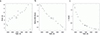 |
Fig. 1. Temperature distributions for the Hyades in our sample. a. Versus rotation period. The target in the lower right corner is the cool M dwarf binary RSP 348 (not included in the other panels). b. Versus radius as obtained from the Gaia DR3 parallax, and c. versus luminosity L. |
Relevant stellar parameters for our Hyades sample.
All our sample targets are confirmed single-star Hyades members according to four criteria. We follow again the notations by Douglas et al. (2019) and verify single-star compliance with four yes/no (Y/N) flags in Table C.1 in column “Single?”. The four flags stand for: (1) RV is with a rms of less than 2 km s−1 of the system velocity, (2) photometry with a deviation in the color-magnitude diagram of less than 0.375 mag, (3) binarity unconfirmed, (4) confirmed Gaia DR2 RV with an error less than 2 km s−1. We note that only the cool M dwarf RSP 348 (r″ = 13.6 mag, V = 14.2 mag) had incomplete information but was, prior to our observations, not proposed nor confirmed as a binary. Our data in Appendix A (Fig. A.1) show it to be a double-lined spectroscopic binary (SB2) and the target was therefore removed from the magnetic sample.
RSP 68 is listed with a M1-3V companion candidate of ≈0.3 M⊙ detected from speckle interferometry (Patience et al. 1998) and AO imaging (Guenther et al. 2005). However, no significant RV variations were found for it by Folsom et al. (2018) and we conclude that it is either a background target or a very long period companion. We thus treat RSP 68 as an effectively single star. Similar may be the case for RSP 133. During a period in 2022 with seeing below or equal to 0.5″, we noted a faint companion on our guider images, approximately 1.3″ away and V ≈ 17 mag. However, Kopytova et al. (2016) found no companion outside of 2.79 AU of RSP 133 in their lucky imaging survey.
4. Census of stellar parameters
4.1. Temperature, gravity, luminosity, and radius
We adopted effective temperatures from Douglas et al. (2019) based on Tycho-2 BV (Høg et al. 2000), GaiaG-band, and 2-MASS JK photometry as the most homogeneous set of measured temperatures. Spectroscopic temperatures are available for only subsets of our targets (Paulson et al. 2003; Dutra-Ferreira et al. 2016; Cummings et al. 2017). The differences between the spectroscopic and the photometric temperatures are typically less than 100 K per star but the deviations are generally larger for the cooler stars with Teff < 5000 K. We note that in the spectroscopic analysis by Schuler et al. (2006) they used photometric temperatures from B − V from Allende Prieto & Lambert (1999) and transformed to V − K. Jeffery et al. (2022) presented model-determined temperatures for 88 single Hyads from eight sets of stellar models and compared them with photometric temperatures. It shows basically good agreement but some systematic differences for stars cooler than 5500 K remain.
The luminosity, L, was calculated based on the Gaia DR3 distance together with the apparent V magnitude (mostly from Joner et al. 2006 and the photometric Teff from Douglas et al. 2019). From L and Teff, we derive the radius, R⋆, and the logarithmic gravitational surface acceleration, log g, from the relations L ∝ R2Teff4 and g ∝ M/R2, respectively. Because the latter values are all very close to log g = 4.5 (4.3–4.7), and because its choice is not critical for our differential Stokes analysis, we adopt model atmospheres fixed to log g = 4.50 for all targets except the two M dwarfs RSP 542 and RSP 556 for which we adopt log g = 5.0. Masses (M⋆) were estimated originally by Douglas et al. (2019) based on the Gaia DR2 parallax with the above Teffs and are given for orientation.
4.2. Metallicity
For the stellar metallicity, in particular [Fe/H], we compare to the cluster average value of [Fe/H] = +0.18 ± 0.03 dex from Dutra-Ferreira et al. (2016), that is, a logarithmic abundance of A(Fe)) = 7.62 ± 0.02. It is based on 3D model atmospheres, two optimized line lists (one for NLTE line formation and the other for the cluster giants), and consistently applied to high-quality HARPS (giants) and UVES (dwarfs) spectra at resolutions of 110 000 and 60 000, respectively. Three giants and 14 dwarfs were analyzed. The metallicity reported earlier by, for example, Paulson et al. (2003) is about 2σ smaller, +0.13 ± 0.01 dex, but judged compatible with the Dutra-Ferreira et al. (2016) value. Metallicities obtained from isochrone fittings show a tendency to even higher values, order +0.25 (Brandner 2023, and references therein). While the best-fit isochrone (710 Myr, [Fe/H] = +0.25) provides a good fit to the upper and lower main sequence, it still underestimates the luminosity of stars in the mass range between ≈0.3–0.85 M⊙.
The metallicities from our lithium fits in Sect. 5.1 are mostly constrained by the Fe I 6707.43 Å line blend and, with decreasing temperature, by an increasing amount of TiO. For the very cool stars with Teff < 4500 K the atomic transitions do not provide reliable metallicities from Fe anymore. Our iron abundances for these targets in Table 2 are thus unrealistic, as one can already see by the χ2 fit values. A complete chemical abundance analysis including molecular contributors is beyond the scope of this paper. We note that the [Fe/H] errors in Table 2 are internal fitting errors and rather small. Their absolute (external) errors are likely a factor ten larger mostly due to the expected continuum-setting uncertainties. The unknown continuum suppression by molecular lines appears also the reason why the fits adopt increasingly lower metallicities the cooler the target (some even with subsolar [Fe/H]). It is an artifact from the continuum suppression likely due to an overestimation of some of the TiO molecular line opacities. The averaged relative iron abundance of our sample is +0.186 ± 0.045 (rms) when excluding the TiO-dominated stars with Teff < 4500 K. This value agrees very well with the canonical metallicity of +0.18 from Dutra-Ferreira et al. (2016).
LTE lithium and iron abundances.
4.3. Rossby number
The Rossby number, Ro, has become an accepted independent variable against which various activity indicators for cool stars are assessed (e.g., Noyes et al. 1984; Durney & Latour 1978). It is also a parameter in dynamo models and compares timescales between the Coriolis force and the advection. In the present paper, we calculate semi-empirical values as Ro = P/τc, where P is the rotation period of the star, and τc is the convective turnover timescale. We use the convective turnover timescales listed in Table 1 of Barnes & Kim (2010), interpolating as needed from the stellar effective temperatures, specifically the global one, representing an average over the entire convection zone. While it is true that different tabulations of τc list differing values, there is largely only a scaling difference between them, so that the power-law relations that characterize variables against Ro are unaffected. To remove the bulk of the differences in Ro that is incurred from the choice of a particular source for the convective turnover timescales, we further normalize the values of Ro by the respective solar value (Ro⊙ = 0.747 using P⊙ = 26.09 d and τc⊙ = 34.9 d). It provides values of Ron = Ro/Ro⊙. This has the effect of translating the numerical value of the solar Ro from 0.75 to exactly 1.00, facilitating inter-comparisons between our work and others that might use alternative convective turnover timescales (e.g., Mathur et al. 2025). These values are listed in Table 1, and used in the figures in this paper.
4.4. Projected rotational velocity and inclination
Another set of stellar parameters concerns the line broadening, mainly the rotational velocity, v sin i, the micro turbulence, ξt, and the (radial-tangential) macro turbulence, ζt. We adopt canonical values for ξt from (Dutra-Ferreira et al. 2016, their Table 5) and for ζt from (Gray 2022, his Table B.1) but redetermine v sin i from our R = 130 000 spectra. Involved is here the inclination, i, of the stellar rotational axis with respect to the line of sight. It remains a weakly constrained parameter. Only for RSP 198 and RSP 68 measured i values from ZDI are available from Folsom et al. (2018) of  ° and
° and  °, respectively. We measure v sin i by means of an autocorrelation function (ACF) technique employing the large wavelength ranges available from CD3 and CD5. An ACF is computed from phase-combined spectra only; these combined spectra are build from all individual (phase-resolved) spectra by averaging them with equal weight to a single spectrum per target of very high S/N of typically 2000:1 per pixel. We note that the lithium analysis in Sect. 5.1 also uses these combined spectra and lists the combined S/N values in Table 3. Wavelength ranges for the autocorrelation mask exclude regions with telluric contamination and strong lines like, for example, Hα in the red CD or the Mg I triplet in the blue CD. The width of the ACF is then deconvolved from the combined instrumental profile and adopted macroturbulence listed in Table 1 with a two-piece linear fit to its FWHM versus Teff (one fit for Teff ≤ 4000 K, one for Teff > 4000 K). This approach basically follows the technique used by Fekel (1997). A formal error is computed from the squared sums of the ACF width of different wavelength regions plus the O-Cs from the FWHM versus Teff fits but is unrealistically small. Instead, we estimate the real v sin i error to be approximately ±0.3 km s−1 from repeated applications to different wavelength chunks.
Logarithmic Ca II IRT emission-line fluxes and radiative losses.
With the above v sin i values, we estimate the most likely inclination i from the rotation period and the Gaia DR3-based stellar radius in Table 1. Its equal likeliness range is the result from the errors of the parallax and effective temperature, and from v sin i and the period. The inclination is thus a heuristically determined value and not a measurement. The typical uncertainty range is 10–15°, basically driven by the error of Teff and v sin i, which are typically ±50 K and ±0.3 km s−1, respectively. We note that for one target (RSP 556) the v sin i measurement is below our empiric spectroscopic detection limit and accordingly more uncertain. The most likely value for i is given in Table 1.
4.5. Radial velocity
The radial velocities in this paper were determined in the course of building the LSD line profiles from Stokes I and V spectra for the magnetic field measurements and were zeroed by the standard Th-Ar calibration. Our spectra are on average 445 ± 278(rms) m s−1 higher than the Gaia DR3 velocities (Katz et al. 2023). The 445 m s−1 difference is just a zero-point difference and can be corrected for if desired. The annual RV stability of PEPSI is estimated to be around 6–10 m s−1. While relative RVs during one night can be of even higher precision, the above large rms of 278 m s−1 indicates that it is the rotational modulation of the surface activity and the time coverage of our sample that set the external RV accuracy. The RVs in Table 1 are phase averages from all spectra available. All targets exhibit modulation of the RVs due to spots and other surface inhomogeneities in the range of above rms value.
5. Surface activity measurements
5.1. Lithium abundance
We employed Turbospectrum (Plez 2012) and its fitting program TurboMPfit (Steffen et al. 2015) for a direct line synthesis fit of the wavelength region 6706–6709 Å. Our fits are based on a predetermined set of 1D LTE spectra synthesized from MARCS (Gustafsson et al. 2008) model atmospheres for different effective temperatures Teff, gravities log g, relative metallicities [Fe/H], microturbulence velocities ξt, lithium abundances A(Li), and isotope ratios 6Li/7Li. TurboMPfit compares then the observed spectrum with the library spectra to find the best match based on a chi-square minimization. For numerical details, we refer to the descriptions in Strassmeier et al. (2023). All abundances in this paper were determined from the phase-averaged spectra with exceptionally high S/N, varying from 628 (RSP 556) to 3296 (RSP 177). Figure 2 shows a zoom into the Li region for all stars. The detailed fits are shown in Fig. B.1. Figure 3 is an example (RSP 177, Teff = 5770 K) for the expected changes in the line core due to rotational modulation and/or cyclic variability, if present. Table 2 provides the total lithium abundance A(Li) according to Eq. (1) and the 6Li/7Li isotopic ratio whenever detected,
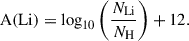 (1)
(1)
As the line list we adopted the list from Strassmeier & Steffen (2022), which is based on Meléndez et al. (2012), except for the Li doublet with isotopic hyperfine components and the broadening constants, and the vanadium blend at 6708.1096 Å (Lawler et al. 2014). Also added are lines of the TiO molecule of five Ti isotopes from the updated list based on Plez (1998). The free parameters are A(Li), 6Li/7Li, [Fe/H], a global wavelength adjustment, and a global Gaussian line broadening (FWHM), which are applied in velocity space to the synthetic interpolated line profiles to match the observational data as closely as possible. FWHM represents the full width half maximum of the applied Gaussian kernel and represents the combined instrumental plus (Gaussian) macro turbulence broadening. We note that we had to allow TurboMPfit to alter the continuum level as well. This has practically no impact for the minimization process for stars warmer than Teff ≈ 5000 K but is needed for the coolest targets due to the dramatically increased molecular suppression of the continuum once Teff < 4500 K. The micro turbulence remained fixed to the values in Table 1.
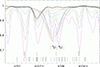 |
Fig. 2. Comparison of the lithium 6707.8-Å region for our sample stars. We show the phase-combined spectra. The short vertical dashes indicate the wavelengths of blending lines. The bottom row of dashes shows the line list from Strassmeier & Steffen (2022), the middle row shows the strongest CaH and TiO lines from the solar umbral atlas, and the upper four dashes indicate the two 7Li and 6Li doublets, respectively. The x-axis is the wavelength in Ångstroem. |
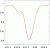 |
Fig. 3. Nineteen individual Li I 6707.8-Å line profiles of RSP 177 (Teff = 5770 K). It indicates the expected range of line-core changes over time. The black profiles are from 2020 (season S20), and the red profiles are from 2022 (season S22), according to Table C.1. The maximum line-core variability in this case is 0.8%. The x-axis is the wavelength in Ångstroem. |
TurboMPfit fitting errors are interpreted as internal errors and are also listed in Table 2. The related χ2 from the fit range 6707.3–6708.5 Å (covered by 44 CCD pixels) is a good indicator for the reliability of the Li abundance but strongly depends on the completeness of the line list. The present high data quality excludes the limited S/N as the (usual) dominant error source. We note that the reason for the larger than expected χ2 with respect to the S/N values is certainly not some unknown systematics in the stellar spectra but is rather related to the imperfect model (synthetic spectra) we are using for fitting. We conclude that the external errors of our Li abundances are almost exclusively driven by the uncertainty of the stellar effective temperature, and only for the coolest stars also by the blending line list. Due to the increasing molecular contribution with lower temperature, the line list becomes more critical the cooler the target. Our line list allows excellent line-profile fits to within the present data quality for Teff > 4500 K but basically fails for Teff < 4200 K. Cummings et al. (2017) had also noted that their errors in A(Li) that result from errors in Teff go fairly parallel to the A(Li) versus Teff trend in the sense the cooler the target the higher the uncertainty. We refer to their discussion and to Dumont et al. (2021) for a general summary of the extensive open cluster Li data including the Hyades.
We estimate external abundance errors by redoing the fits for all targets but with Teff ± 100 K with respect to the nominal value. The maximum/minimum range for A(Li) and [Fe/H] is then adopted as a more realistic estimate of their true error. For A(Li), we obtain ±0.08 to ±0.15 for Teff ≈ 6000 K to ≈4500 K, respectively. For [Fe/H], we obtain ±0.05 to ±0.01 for the same Teff range (smaller errors for the cooler stars in this case).
The only stars for which the formally best fit required 6Li were RSP 134, 439, 95, 429, and 216. Their isotopic ratios are between 10–15% (Table 2). However, we deem none of them to be a real detection and attribute all Li to 7Li. This is because the formal fitting errors provided by the Levenberg-Marquard algorithm are not relevant in this case because uncertainties are driven by the uncertainties of the line list rather than the fit to the data. The 7Li abundances range from a high of +3.01 (RSP 340, Teff = 6158 K) to a low of negative (logarithmic) values for the most cool targets. The latter are then just upper limits. 3D NLTE corrections are not available for all temperatures of our Hyades dwarfs and could thus not be applied uniformly. All Li abundances in this paper are thus LTE abundances. The real uncertainties for the targets with very low A(Li) values, basically all targets cooler than 4200 K, are again driven by the molecular contamination (due to imperfect continuum setting, line profile blending, and partly wrong line parameters) and are merely estimates.
5.2. Chromospheric Ca II IRT flux
We measured the absolute line-core flux, ℱ, in the Ca II infrared triplet from our CD VI spectra at 8498, 8542 and 8662 Å (dubbed IRT-1, IRT-2, and IRT-3, respectively). The central portions of these spectra are visualized in Fig. B.2. Fluxes in erg cm−2 s−1 were computed from the measured relative flux in a 1-Å band centered on the line core and scaled with the absolute continuum flux at these wavelengths. The latter is obtained for the B − V range of our targets from the relations provided by Hall (1996). We followed the same procedure as in our recent spectroscopic survey of the ecliptic poles (Strassmeier et al. 2023) or our search for Maunder-minimum candidates Järvinen & Strassmeier (2025) and refer to these papers for details.
The total atmospheric radiative loss in the Ca II IRT, RIRT, is determined from the sum of the absolute fluxes from the three lines in units of the stellar bolometric luminosity σTeff4,
 (2)
(2)
It is an indicator of the stellar atmospheric magnetic activity, photosphere and chromosphere combined. We also provide the chromospheric radiative loss, R′IRT, by removing the expected photospheric contribution from the individual fluxes via bona-fide inactive stars. Such a correction is not unproblematic because it always makes the idealized assumption that inactive stars come without a chromosphere and that the photospheric contribution of these stars is unrelated to its activity, thus will introduce unspecified additional uncertainty. Nevertheless, Martin et al. (2017) provided a convenient collection of such corrections based on 26 bona-fide inactive stars as a function of B − V and v sin i. These spectra were taken at a spectral resolution of ∼20 000 which is, however, over six times lower than the resolution of our present Hyades spectra. Järvinen et al. (2016) had provided IRT corrections based on 52 inactive stars observed with STELLA at a spectral resolution of 55 000. For the B − V range of our Hyades sample, these corrections are on average 4–5% lower than the ones by Martin et al. (2017). Although this is only a small amount well within the expected flux uncertainties, the difference is systematic and likely due to the different spectral resolution (see Järvinen & Strassmeier 2025, for more details). Numerical photospheric corrections are between 1 × 10⁶ and 6 × 10⁶ erg cm−2 s−1 for the sum of all three IRT lines for B − V of 1.4–0.6 mag, respectively. Table 3 lists the corrected radiative losses based on the Järvinen et al. (2016) correction along with the uncorrected fluxes. We refrain from further corrections, for example of the basal flux due to acoustic heating (c/o Shrijver 1995, see discussion in Martin et al. 2017). In any case the photospherically corrected radiative losses are an indirect measure of the magnetic flux from the chromosphere.
Because only a single spectrum per target with CD VI is available, our fluxes are just snapshots from the range of expected variability due to rotational modulation. Measuring errors for RIRT are driven by the error for Teff and B − V and are not explicitly listed in the table but are estimated to be of the order of 10–20% following the Teff evaluation in Cummings et al. (2017) and Douglas et al. (2019). We expect rotational IRT flux modulation that is significantly smaller than ≈15% (as measured for the RS CVn binary λ And; Adebali et al. 2025).
5.3. Magnetic field measurements
We first reconstructed the Stokes-V LSD spectral lines from the combined spectra from CD III and CD V. Figure 4a shows a comparison of the LSD Stokes-V (and Stokes-I) profiles for one representative target (RSP 177, Teff = 5770 K). These LSD profiles are then converted to a disk-integrated Stokes-V profile in units of Gauss (Fig. 4b) following the procedure laid out in Kochukhov et al. (2010) based on the earlier notions from Solanki & Stenflo (1984). Spectral lines for the deconvolution were selected from the most-recent version of the Vienna Atomic Line Database (VALD-3; Ryabchikova et al. 2015) based on line strength, Landé factor, and blending. The number of available lines varies with stellar effective temperature and ranges from a minimum of 3326 for RSP 340 to 27 158 for RSP 542.
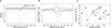 |
Fig. 4. Representative Stokes-V data and results for RSP 177. a. Top spectra: All available 19 LSD Stokes-V line profiles are overplotted in units of the continuum expanded by a factor 100 and shifted in intensity by 0.1 for better visibility. Bottom spectrum: Example LSD Stokes-I profile. b. Phase-resolved disk-integrated Stokes-V LSD line profiles in units of Gauss. c. Longitudinal magnetic field versus rotational phase. Indicated are the two observing seasons for this target (S22: filled dots, S20: rings). The appendix provides similar figures for the other targets (Fig. B.3). |
The LSD wavelength integration gives the longitudinal field component Blong, with either positive or negative polarity (Fig. 4c) by assuming the standard weak-field approximation (e.g., Stenflo 1989). Its absolute value, |B|, is obtained by integrating the positive and negative polarities and is commonly called the “unsigned” magnetic field. Longitudinal fields are extracted for every available LSD Stokes-V line profile. Individual errors typically range from ±0.7 G to ±1.0 G for the majority of targets depending on the number of available lines and the S/N per pixel. The five targets with Teff < 4500 K have errors of up to ±10 G. Rotational phases, φ, were calculated with the respective rotation periods from Table 1 and an arbitrary zero point assumed to be the time of the first integration of our first Hyades target; BJD 2 459 185.7700 (= Dec. 2, 2020). Whenever there is more than one period determination, we preferred the period from K2 data or, if no K2 period was available, the one with the smaller error. For the six stars where this is the case the period used is the one listed in Table 1 and referenced in Table C.1. Phase gaps due to bad weather are unavoidable on Mt. Graham and are identified in the last three columns of Table C.1. We consider the phase coverage “partial” (indicated there by a letter P) if a gap of ≥0.30 phases exists.
Figure 4c shows the phase variations of the measured longitudinal fields for one example target; RSP 177. Plots for the other targets are collected in Fig. B.3. We apply a simple harmonic (multi-periodic) fit to all rotationally-phased measurements of all targets in order to estimate the distribution of isolated polarities, dubbed magnetic spots. From Fig. B.3, we see that most of our targets exhibit a relatively high frequency of variability during a rotation cycle. Among the most extreme are RSP 134 with four maxima (i.e., positive polarity dominating) and four minima (negative polarity dominating) and RSP 177 in 2020 with only one maximum and one minimum. This is not unexpected when compared to the Sun. In a recent technical paper on Sun-as-a-star Stokes-V polarimetry with PEPSI (Strassmeier et al. 2024), we observed changes of the shape of its Stokes-V line profile within four days (≈0.15 rotational phases; also with the same sampling of one spectrum per day) due to the change in dominance from positive to negative polarities and back again. Our more active Hyads apparently show a similar and likely even quicker variability than the current Sun.
Table 4 lists the mean longitudinal fields observed from the available data sets, ⟨Blong⟩, its variability amplitude ΔBlong and rms, and the time/phase-averaged unsigned magnetic fields ⟨|B|⟩ with errors. We note that these errors are simply rms values scaled by the square root of the number of available measurements.
Magnetic field strengths.
6. Hyades activity-rotation relations
6.1. Lithium dependence
The high resolution and S/N of our data allow a new look at the Li dependence on stellar Teff and Prot for the age of the Hyades. Cummings et al. (2017) had already found a very tight A(Li) versus Teff relation for the Hyades G dwarfs (5400–6200 K) from their WIYN/Hydra sample of 34 targets. These data had a comparably low resolution of 13 500 but high S/N of typically several hundreds. For a direct comparison with our data, we have 8 targets in common (RSP 137 = vB10, RSP 177 = vB15, RSP 225 = vB26, RSP 227 = vB27, RSP 233 = vB31, RSP 340 = vB65, RSP 344 = vB66, RSP 440 = vB97). Their individual A(Li) differences scatter with a rms of 0.06 dex with an average difference of just 0.016 dex (ours on average lower with respect to Cummings et al.). While Cummings et al. obtained A(Li) from individual spectra, our A(Li) are from phase-averaged spectra. As we have shown in Fig. 3 for one target (RSP 177), the line-core changes due to rotational modulation are very small (typically < 0.8%) and impact on A(Li) only on the one-percent level. From this, we conclude that no zero-point shift between our two data sets must be applied despite of the time difference of the observations of more than a decade.
The first column in the matrix-like Fig. 5 shows plots of A(Li) versus Teff (Fig. 5a), Prot (Fig. 5b), v sin i (Fig. 5c), and Ron (Fig. 5d). Quite intriguing is the tight relation of A(Li) with Teff for our full temperature range from 6160 K to 3780 K, and not just for the G dwarfs as demonstrated by Cummings et al. (2017). We do not observe a continuous steep depletion trend for the stars cooler than approximately 5000 K but more a weakened decrease towards a lower limit at around 1/25 (≈ − 0.4 dex) of the solar A(Li). Such a depletion change and minimum abundance, if real, remains unexplained in the standard Li isochrones (referring to the reviews by Pinsonneault (1997) and Bouvier (2020), that is, models without rotation, diffusion, mass loss, etc.) but had already been noted in the early Li study by Thorburn et al. (1993). Whether the abundance raeches truly zero or some sort of a minimum steady-state abundance remains undetermined from our spectra because of the uncertain molecular contribution to the synthesis line list. The A(Li) values for the four coolest stars in our sample, and in particular the most cool target (RSP 556; Teff = 3780 K, A(Li) ≈ –1) are thus likely upper limits. For these, we estimate a more realistic ±0.3 dex internal uncertainty, which then would transform to a possible steady-state limit of the above mentioned ≈1/25 of the solar Li abundance. The Li-Teff relation from Cummings et al. (2017) already demonstrated the significant surface depletion down to solar levels for the late G dwarfs around 5400 K. Our G-M star abundances verify and extend this trend and the current observations may indicate a minimum Li level for stars cooler than 4100 K (M1 or ≈0.5 M⊙). Its interpretation is pending but could be related to a minimal efficiency of the transportation capacity of the internal mixing process.
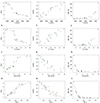 |
Fig. 5. Lithium-activity-rotation relations. The figure compares various relations in a matrix form (columns vs. rows) of A(Li), R′IRT, and ⟨|B|⟩ (from left to right) vs. Teff, Prot, v sin i, and Ron (from top to bottom). Fits are shown for the panels for Rossby-number dependence. The line in panel l is a combined and interpolated fit from the two-piece linear fit in Eq. (6). |
Is there also a dependence of A(Li) on stellar rotation? The common understanding is that faster-rotating stars lose more angular momentum and accordingly induce greater internal mixing and thus surface Li depletion (e.g., Butler et al. 1987; Balachandran et al. 1988; Soderblom et al. 1993; Bouvier et al. 2018; Llorente de Andres et al. 2021). This is what is seen for Hyades stars cooler than the Li dip (G dwarfs and cooler) where higher A(Li) is measured for the faster rotators. We note that Boesgaard’s (1987) study of Hyades F dwarfs showed that the decline in v sin i from Teff of 6600 K to about 6300 K coincided with an increase in A(Li), that is, an inverse rotation-lithium relation leading to a second A(Li) maximum near 6200 K in the A(Li) versus Teff plane (stars cooler than ≈6000 K were not covered then). More recently, Takeda et al. (2013) investigated 68 Hyads warmer than 5100 K at high spectral resolution (R ∼ 67 000) which they used to also search for a v sin i dependence. They concluded that A(Li) in their sample is essentially controlled by Teff and shows no positive correlation with stellar rotation. However, the rotational velocity range of their studied subsample with Teff < 6000 K was just 3.5–6.0 km s−1. This finding would be somewhat in contradiction with the finding of Llorente de Andres et al. (2021) of a minimum (critical) rotational velocity of ≈5 km s−1 that separates Li-rich from Li-poor stars at A(Li) ≈ 2.5. Their sample included field stars as well as open-cluster stars from many different sources. Our Hyades sample shows the same strong A(Li)-Teff dependence as found previously but also a clear relation to rotation described by the three functionals v sin i, Prot, and Ron, themselves implicitly related to Teff and radius though. A second order polynomial fit to A(Li) versus Ron in Eq. (3) gives
 (3)
(3)
This fit is shown in Fig. 5d as a solid line quantifying higher lithium abundance for targets with larger Rossby numbers. Figure 5b shows the commonly recognized behavior once rotation period is plotted alone, that is, higher lithium abundance for the faster rotating targets, basically the same behavior than for v sin i in Fig. 5c. The inverse trend with Rossby number in Fig. 5d thus just reflects that the respective convective turn-over times dominate over the rotational periods. While the latter span in our target sequence from 5 to 16 d, that is a factor three, the convective turn-over times (τ in Table 1) span over a factor 14. Therefore, the plot versus rotation period (Fig. 5b) mirrors just the temperature dependence while the v sin i plot mirrors the true rotational dependence. We also note that Fig. 5c indicates a v sin i distribution with a critical velocity at ≈6.0 km s−1 (Prot ≈ 8 d, Ron ≈ 0.4) and A(Li) of 2.6, where “critical” is defined as the onset of the A(Li) plateau towards higher rotation. This is in good agreement with the observations of Llorente de Andres et al. (2021). However, we emphasize that our sample is still restricted to v sin i between 1–10 km s−1 (periods between 5–16 d) and thus does not cover the full Li plateau.
6.2. Chromospheric activity dependence
Compared to the range of three orders of magnitude for A(Li), the Ca II IRT radiative losses span only one order of magnitude. Independent of a photospheric correction, it indicates the relative increase of the chromospheric contribution as one goes from late-F/early-G stars to early M-stars.
The second column in Fig. 5 plots the photospherically corrected radiative loss R′IRT versus Teff (Fig. 5e), Prot (Fig. 5f), v sin i (Fig. 5g), and Ron (Fig. 5h), respectively. We recall that  was computed from all three Ca II IRT lines subtracted by the respective photospheric flux and normalized to the bolometric luminosity in logarithmic form. It indicates the reaction of the chromosphere on the presence of a permeating magnetic field.
Fritzewski et al. (2021) had demonstrated a tight R′IRT versus Ro relation for the 300 Myr open cluster NGC 3532. This cluster is more than two times younger than the Hyades and its chromospheric IRT radiative losses on average two-and-a-half times larger (≈0.4 dex) than the ones we measured for the Hyades. NGC 3532 stars with Ro > 0.06 (and less than ≈0.2) were defined as unsaturated and fitted with a linear function (Eq. (4) in Fritzewski et al. 2021). This fit is partly outside of our Hyades Ro range of 0.1–0.4 and is thus difficult to compare. Nevertheless, a similar linear fit to the Hyades versus unnormalized Rossby numbers like in Fritzewski et al. (2021) is given in the following Eq. (4):
 (4)
(4)
It shows basically good agreement for the overlapping Ro regime but with the above mentioned offset in R′IRT of ≈–0.4 dex for the Hyades. A full-range second-order polynomial fit, like for A(Li) in Eq. (3), is applied to the normalized Rossby numbers (Ron) and is given in Eq. (5),
 (5)
(5)
Figure 5e shows a remaining temperature dependence even after photospheric correction verifying that the cooler targets tend to have more active chromospheres. It is basically mirrored into the rotation-period dependence (Fig. 5f): Hyads with longer rotation periods exhibit higher chromospheric IRT losses, which is a sort-of inverse rotation-activity relation. However, this is driven by the natural dependence of τ on Teff because the longer-period targets are also the coolest.
The dependence on projected rotational velocity (Fig. 5g) is comparable and in the sense higher radiative losses are seen for targets with lower rotational velocities. The latter is also opposite to what is seen for A(Li) where higher abundances are seen for the targets with higher rotational velocities. The v sin i dependence of R′IRT is again mirrored in the one versus Rossby number in Fig. 5h, that is, higher radiative losses for targets with smaller Rossby numbers, which follows the expected rotation-activity relation for unsaturated stars. It is worth noting here that the three relations versus v sin i in Figs. 5cgk are qualitatively the same if plotted versus angular momentum instead. We recall that the latter (MRv) explicitly includes the masses, radii, and the most probable inclinations of the rotational axis, i, from Table 1.
6.3. Magnetic field dependence
The longitudinal component of the large-scale surface magnetic field of our Hyads is reconstructed as a function of rotational phase from Stokes-V LSD line profiles. Because an LSD profile could be considered a mean photospheric line, our magnetic field measurements are thus for a mean photosphere. At this point, we (re)emphasize that CP-based data measure the topological field strengths rather than the expectedly much higher local field strengths and thus much better represent the global scale of the field. However, the disk averaging makes it prone to flux cancellation in regions of opposite magnetic polarity within a surface resolution element. Among a subsample of slowly rotating M stars, Reiners et al. (2022) showed that the surface averaged small-scale magnetic field strength is proportional to Rossby number, and thus in qualitative agreement with the global-scale field from polarimetric spectra, albeit with higher field strengths by a factor of ten compared to polarimetric data. The underlying cause for a correlation with rotation and age is the magnetic field decay as stars age and rotation decreases. As emphasized in the review by Linsky (2017) it is difficult to quantify these relations as they likely depend also on local magnetic field strength and corresponding magnetic energy which usually can only be directly measured on the Sun. An actual relation between local and global field remains an open dynamo flux-transport issue (see, e.g., Brun et al. 2022).
We obtained longitudinal field strengths in the range −100 G (e.g., RSP 542) and +150 G (e.g., RSP 409 and 571), converted to unsigned average fields ranging between 11.4 and 217 G, thus covering rougly a range of a factor twenty. One target, RSP 556, was observed with only positive polarity but had two significant phase gaps which prevented complete surface visibility. For the two targets in common with the study of Folsom et al. (2018), RSP 68 = Mel25-5 and RSP 198 = Mel25-21, we measured approximately twice as high Blong values: 20 G with a range of 46 G (compared to Folsom et al. 2018 of 11 G with a range of 15 G) and 35 G with a range of 43 G (compared to 14 G with range 18 G), for the two targets, respectively. We note that there were seven years in between our observations and those of Folsom et al. (2018). The surface-averaged unsigned magnetic field strengths for above two targets are nevertheless quite comparable: 13.0 G versus 13.0 G, and 17.6 versus 12.7 G, for ours versus (Folsom et al. 2018), respectively. For target-to-target comparisons prior to ZDI in this paper, we thus focus on the unsigned average fields listed in Table 4 in column ⟨|B|⟩.
The third column in the matrix figure Fig. 5 plots the phase-averaged unsigned field strength ⟨|B|⟩ versus Teff (Fig. 5i), Prot (Fig. 5j), v sin i (Fig. 5k), and Ron (Fig. 5l), from left to right, respectively. It is obvious that it is the coolest and smallest stars that exhibit the strongest surface-averaged large-scale field densities (as well as higher chromospheric radiative losses). In our sample it is the slow rotators defined by small v sin i and large Prot that appear with higher global field densities and thus present us an apparent inverse rotation-activity relation. This is also seen in the Ro-panel in Fig. 5l where the coolest stars with the longest rotation periods are the ones with the lowest (normalized) Rossby numbers (Ron ≈ 0.2) and highest field densities. Usually, smaller Rossby numbers indicate faster surface rotation. However, the ⟨|B|⟩ − Ron relation in Fig. 5l appears bimodal with two slopes. A more or less constant (or only slightly decreasing) field density for Ron ≥ 0.25 with an average of 15.4 ± 3.6(rms) G, and a steeply increasing field density for Ron < 0.25 with an average of 91 ± 61(rms) G. We quantify it with a two-piece linear fit in Eq. (6),
 (6)
(6)
At this point, it may be worth mentioning that our sample contains six stars of roughly the same effective temperature around 5000 K (4700-5200 K) but with rotation periods between 9.10 d (RSP 134) and 12.64 d (RSP 216). While the mean longitudinal surface magnetic field, ⟨|B|⟩, is relatively small for all of them (≈18 ± 4 G), its individual variability amplitudes increase from 45 G (RSP 134) to 84 G (RSP 216) towards the slower rotators, that is, nearly a factor two. It not only suggests that ⟨|B|⟩ may be a too simplified parameter for the quantification of a stellar magnetic field but, more importantly, that there is a remaining weak (inverse) rotational dependence also for the stars with Ron ≈ 0.25 (spectral type ≈K1).
7. Summary and conclusions
The basis of our analysis were high-resolution spectra with a high-S/N that allowed the precise determination of three distinct surface-activity tracers for each of the 21 sample dwarfs. The three tracers were the lithium abundance, A(Li), the radiative loss in the chromospheric emission lines of the Ca II infrared triplet, R′IRT, and the average unsigned surface magnetic field strength, ⟨|B|⟩. All three parameters were found to vary with other observables, Teff, Prot, and v sin i, but not in the same way. Our initial target selection of Hyades dwarfs implicitly sampled a stellar mass sequence (and thus, also a radius and Teff sequence) at an age of ≈700 Myr and at a supersolar metallicity of +0.18. We thus expected parameter dependences along this sequence. The addition of rotational parameters made this a true Rossby-type sequence.
In particular, we found a clear Rossby-number dependence of A(Li), R′IRT, and ⟨|B|⟩. Only A(Li) increases with increasing Rossby number, however, while the other two parameters basically decline with increasing Rossby number. At the same time, A(Li) also increases with projected rotational velocity, v sin i, and decreases with rotational period, which basically reflects the mass-radius dependence of the Rossby sequence, while the other two parameters, R′IRT and ⟨|B|⟩, indicate the opposite, that is, a decrease with increasing rotation.
We interpret this in the sense that the observed trend of Li depletion is not primarily caused by some rotation-induced mixing process. The mass dependence of the depth of the outer convection zone instead enforces a mass-dependent Li depletion rate. There is a (surface) rotational and angular-momentum dependence as well, but we argued that rotational mixing exists in parallel, but only modifies the A(Li) versus Teff relation, in particular for the faster rotators. We speculated that the Li dip (at a Teff higher than in our sample) is in some way a complex consequence of rotational mixing.
The dependence of the averaged unsigned magnetic field strength on the Rossby number appears to have two very different slopes in the sense that only the fastest of our generally slow rotators show a clear dependence. Stars with (normalized) Rossby numbers greater than ≈0.25 exhibit weaker fields by a factor of ≈6 on average, and no or only a weak dependence on rotation. The inverse rotation-activity relation likely arises from a change in the surface magnetic field morpholgy with effective temperature or mass taking place at about Ron ≈ 0.25. We will revisit this with our future ZDI. The global surface activity on targets of Hyades age, in particular when they are cooler than ≈5000 K, appears to be dominated by its convective motions, which in our case was expressed by its turnover time, which itself is inversely proportional to the stellar mass and effective temperature and not to stellar rotation.
Data availability
Full Table C.2 is available at the CDS via https://cdsarc.cds.unistra.fr/viz-bin/cat/J/A+A/704/A8
Acknowledgments
We thank an anonymous referee for the many very helpful suggestions. It is a pleasure to thank the German Federal Ministry (BMBF) for the year-long support for the construction of PEPSI through their Verbundforschung grants 05AL2BA1/3 and 05A08BAC as well as the State of Brandenburg for the continuing support of AIP and PEPSI for the LBT (see https://pepsi.aip.de/). The LBT is an international collaboration among institutions in the United States, Italy and Germany. LBT Corporation partners are: The University of Arizona on behalf of the Arizona Board of Regents; Istituto Nazionale di Astrofisica, Italy; LBT Beteiligungsgesellschaft, Germany, representing the Max-Planck Society, The Leibniz Institute for Astrophysics Potsdam, and Heidelberg University; The Ohio State University, representing OSU, University of Notre Dame, University of Minnesota and University of Virginia. This work has made use of NASA’s Astrophysics Data System and of CDS’s Simbad database which we all gratefully acknowledge.
References
- Adebali, Ö., Strassmeier, K. G., Ilyin, I. V., et al. 2025, A&A, 695, A89 [NASA ADS] [CrossRef] [EDP Sciences] [Google Scholar]
- Adibekyan, V., Sousa, S. G., Santos, N. C., et al. 2020, A&A, 642, A182 [NASA ADS] [CrossRef] [EDP Sciences] [Google Scholar]
- Allende Prieto, C., & Lambert, D. L. 1999, A&A, 352, 555 [NASA ADS] [Google Scholar]
- Balachandran, S., Lambert, D. L., & Stauffer, J. R. 1988, ApJ, 333, 267 [NASA ADS] [CrossRef] [Google Scholar]
- Barnes, S. A. 2003, ApJ, 586, 464 [Google Scholar]
- Barnes, S. A. 2007, ApJ, 669, 1167 [Google Scholar]
- Barnes, S. A., & Kim, Y.-C. 2010, ApJ, 721, 675 [Google Scholar]
- Boesgaard, A. M. 1987, PASP, 99, 1067 [Google Scholar]
- Bouvier, J. 2020, Mem. Soc. Astron. It., 91, 39 [NASA ADS] [Google Scholar]
- Bouvier, J., Barrado, D., Moraux, E., et al. 2018, A&A, 613, A63 [NASA ADS] [CrossRef] [EDP Sciences] [Google Scholar]
- Brandner, W., Calissendorff, P., & Kopytova, T., 2023, MNRAS, 518, 662 [Google Scholar]
- Brun, A. S., Strugarek, A., Noraz, Q., et al. 2022, ApJ, 926, 21 [NASA ADS] [CrossRef] [Google Scholar]
- Butler, R. P., Cohen, R. D., Duncan, D. K., & Marcy, G. W. 1987, ApJ, 319, L19 [NASA ADS] [CrossRef] [Google Scholar]
- Carroll, T. A., Kopf, M., Ilyin, I., & Strassmeier, K. G. 2007, Astron. Nachr., 328, 1043 [NASA ADS] [CrossRef] [Google Scholar]
- Corsaro, E., Bonanno, A., Mathur, S., et al. 2021, A&A, 652, L2 [NASA ADS] [CrossRef] [EDP Sciences] [Google Scholar]
- Cummings, J. D., Deliyannis, C. P., Maderak, R. M., & Steinhauer, A. 2017, AJ, 153, 128 [Google Scholar]
- Delorme, P., Collier Cameron, A., Hebb, L., et al. 2011, MNRAS, 413, 2218 [Google Scholar]
- Donati, J.-F., Semel, M., Carter, B. D., Rees, D. E., & Collier Cameron, A. 1997, MNRAS, 291, 658 [NASA ADS] [CrossRef] [Google Scholar]
- Douglas, S. T., Agüeros, M. A., Covey, K. R., et al. 2014, ApJ, 795, 161 [NASA ADS] [CrossRef] [Google Scholar]
- Douglas, S. T., Agüeros, M. A., Covey, K. R., et al. 2016, ApJ, 822, 47 [NASA ADS] [CrossRef] [Google Scholar]
- Douglas, S. T., Curtis, J. L., Agueros, M. A., et al. 2019, ApJ, 879, 100 [NASA ADS] [CrossRef] [Google Scholar]
- Dumont, T., Charbonnel, C., Palacios, A., & Borisov, S. 2021, A&A, 654, A46 [NASA ADS] [CrossRef] [EDP Sciences] [Google Scholar]
- Durney, B. R., & Latour, J. 1978, Geophys. Astrophys. Fluid Dyn., 9, 241 [Google Scholar]
- Dutra-Ferreira, L., Pasquini, L., Smiljanic, R., Porto de Mello, G. F., & Steffen, M. 2016, A&A, 585, A75 [NASA ADS] [CrossRef] [EDP Sciences] [Google Scholar]
- Fan, Y. 2009, Liv. Rev. Sol. Phys., 6, 4 [Google Scholar]
- Fekel, F. C. 1997, PASP, 109, 514 [NASA ADS] [CrossRef] [Google Scholar]
- Folsom, C. P., Bouvier, J., Petit, P., et al. 2018, MNRAS, 474, 4956 [NASA ADS] [CrossRef] [Google Scholar]
- Fritzewski, D. J., Barnes, S. A., James, D. J., Järvinen, S. P., & Strassmeier, K. G. 2021, A&A, 656, A103 [NASA ADS] [CrossRef] [EDP Sciences] [Google Scholar]
- Gaia Collaboration (Babusiaux, C., et al.) 2018, A&A, 616, A10 [NASA ADS] [CrossRef] [EDP Sciences] [Google Scholar]
- Gaia Collaboration (Vallenari, A., et al.) 2023, A&A, 674, A1 [NASA ADS] [CrossRef] [EDP Sciences] [Google Scholar]
- Garraffo, C., Drake, J. J., Dotter, A., et al. 2018, ApJ, 862, 90 [NASA ADS] [CrossRef] [Google Scholar]
- Gray, D. F. 2022, The Observation and Analysis of Stellar Photospheres, 4th edn. (Cambridge University Press) [Google Scholar]
- Guenther, E. W., Paulson, D. B., Cochran, W. D., et al. 2005, A&A, 442, 1031 [NASA ADS] [CrossRef] [EDP Sciences] [Google Scholar]
- Gustafsson, B., Edvardsson, B., Eriksson, K., et al. 2008, A&A, 486, 951 [NASA ADS] [CrossRef] [EDP Sciences] [Google Scholar]
- Hale, G. E. 1927, Nature, 119, 708 [Google Scholar]
- Hall, J. C. 1996, PASP, 108, 313 [NASA ADS] [CrossRef] [Google Scholar]
- Høg, E., Fabricius, C., Makarov, V. V., et al. 2000, A&A, 355, L27 [Google Scholar]
- Houdebine, E. R., & Stempels, H. C. 1997, A&A, 326, 1143 [NASA ADS] [Google Scholar]
- Ilyin, I. 2000, Ph.D. Thesis, Univ. of Oulu, Finland [Google Scholar]
- Jardine, M., Vidotto, A. A., van Ballegooijen, A., et al. 2013, MNRAS, 431, 528 [NASA ADS] [CrossRef] [Google Scholar]
- Jardine, M., Vidotto, A. A., & See, V. 2017, MNRAS, 465, L25 [Google Scholar]
- Järvinen, S. P., & Strassmeier, K. G. 2025, A&A, 698, A93 [NASA ADS] [CrossRef] [EDP Sciences] [Google Scholar]
- Järvinen, S. P., Kordopatis, G., Strassmeier, K. G., & Steinmetz, M. 2016, https://doi.org/10.5281/zenodo.57464 [Google Scholar]
- Jeffery, E. J., Taylor, B. J., & Joner, M. D. 2022, ApJ, 936, 153 [Google Scholar]
- Joner, M. D., Taylor, B. J., Laney, C. D., & van Wyk, F. 2006, AJ, 132, 111 [Google Scholar]
- Katz, D., Sartoretti, P., Guerrier, A., et al. 2023, A&A, 674, A5 [NASA ADS] [CrossRef] [EDP Sciences] [Google Scholar]
- Kochukhov, O., Makaganiuk, V., & Piskunov, N. 2010, A&A, 524, A5 [NASA ADS] [CrossRef] [EDP Sciences] [Google Scholar]
- Kochukhov, O., Hackman, T., Lehtinen, J. J., & Wehrhahn, A. 2020, A&A, 635, A142 [NASA ADS] [CrossRef] [EDP Sciences] [Google Scholar]
- Kopytova, T. G., Brandner, W., Tognelli, E., et al. 2016, A&A, 585, A7 [NASA ADS] [CrossRef] [EDP Sciences] [Google Scholar]
- Kraft, R. P. 1967, ApJ, 150, 551 [Google Scholar]
- Kundert, A., Cargile, P. A., Dhital, S., et al. 2012, AAS, 219, 15213 [Google Scholar]
- Lawler, J. E., Wood, M. P., Den Hartog, E. A., et al. 2014, ApJS, 215, 20 [CrossRef] [Google Scholar]
- Lehmann, L. T., Hussain, G. A. J., Vidotto, A. A., Jardine, M. M., & Mackay, D. H. 2021, MNRAS, 500, 1243 [Google Scholar]
- Linsky, J. L. 2017, ARA&A, 55, 159 [Google Scholar]
- Llorente de Andres, F., Chavero, C., de la Reza, R., Roca-Fabrega, S., & Cifuentes, C. 2021, A&A, 654, A137 [NASA ADS] [CrossRef] [EDP Sciences] [Google Scholar]
- Martin, J., Fuhrmeister, B., Mittag, M., et al. 2017, A&A, 605, A113 [NASA ADS] [CrossRef] [EDP Sciences] [Google Scholar]
- Martinez González, M. J., Asensio Ramos, A., Carroll, T. A., et al. 2008, A&A, 486, 637 [NASA ADS] [CrossRef] [EDP Sciences] [Google Scholar]
- Mathur, S., Santos, A. R. G., Claytor, Z. R., et al. 2025, ApJ, 982, 114 [Google Scholar]
- Meléndez, J., Bergemann, M., Cohen, J. G., et al. 2012, A&A, 543, A29 [NASA ADS] [CrossRef] [EDP Sciences] [Google Scholar]
- Mermilliod, J.-C., Mayor, M., & Udry, S. 2009, A&A, 498, 949 [NASA ADS] [CrossRef] [EDP Sciences] [Google Scholar]
- Mestel, L. 1968, MNRAS, 138, 359 [NASA ADS] [CrossRef] [Google Scholar]
- Metcalfe, T. S., Finley, A. J., Kochukhov, O., et al. 2022, ApJ, 933, L17 [NASA ADS] [CrossRef] [Google Scholar]
- Metcalfe, T. S., Strassmeier, K. G., Ilyin, I. V., et al. 2024, ApJ, 960, L6 [NASA ADS] [CrossRef] [Google Scholar]
- Noyes, R. W., Hartmann, L. W., Baliunas, S. L., Duncan, D. K., & Vaughan, A. H. 1984, ApJ, 279, 763 [Google Scholar]
- Parker, E. N. 1958, ApJ, 128, 664 [Google Scholar]
- Patience, J., Ghez, A. M., Reid, I. N., Weinberger, A. J., & Matthews, K. 1998, AJ, 115, 1972 [NASA ADS] [CrossRef] [Google Scholar]
- Paulson, D. B., Sneden, C., & Cochran, W. D. 2003, AJ, 125, 3185 [NASA ADS] [CrossRef] [Google Scholar]
- Perryman, M. A. C., Brown, A. G. A., Lebreton, Y., et al. 1998, A&A, 331, 81 [NASA ADS] [Google Scholar]
- Pinsonneault, M. 1997, ARA&A, 35, 557 [NASA ADS] [CrossRef] [Google Scholar]
- Plez, B. 1998, A&A, 337, 495 [NASA ADS] [Google Scholar]
- Plez, B. 2012, Astrophysics Source Code Library [record ascl:1205.004] [Google Scholar]
- Radick, R. R. 1995, ApJ, 452, 332 [Google Scholar]
- Radick, R. R., Thompson, D. T., Lockwood, G. W., Duncan, D. K., & Baggett, W. E. 1987, ApJ, 321, 459 [NASA ADS] [CrossRef] [Google Scholar]
- Reiners, A., Shulyak, D., Käpylä, P. J., et al. 2022, A&A, 662, A41 [NASA ADS] [CrossRef] [EDP Sciences] [Google Scholar]
- Rosén, L., Kochukhov, O., Hackman, T., & Lehtinen, J. 2016, A&A, 593, A35 [NASA ADS] [CrossRef] [EDP Sciences] [Google Scholar]
- Röser, S., Schilbach, E., Piskunov, A. E., Kharchenko, N. V., & Scholz, R.-D. 2011, A&A, 531, A92 [NASA ADS] [CrossRef] [EDP Sciences] [Google Scholar]
- Rüdiger, G., & Küker, M. 2016, A&A, 592, A73 [NASA ADS] [CrossRef] [EDP Sciences] [Google Scholar]
- Ryabchikova, T., Piskunov, N., Kurucz, R. L., et al. 2015, Phys. Scr, 90, 054005 [Google Scholar]
- Saar, S. H., & Linsky, J. L. 1986, Adv. Space Res., 6, 235 [Google Scholar]
- Schrinner, M. 2011, A&A, 533, A108 [NASA ADS] [CrossRef] [EDP Sciences] [Google Scholar]
- Schuler, S. C., King, J. R., Terndrup, D. M., et al. 2006, ApJ, 636, 432 [Google Scholar]
- See, V., Jardine, M., Vidotto, A. A., et al. 2018, MNRAS, 474, 536 [NASA ADS] [Google Scholar]
- Semel, M. 1989, A&A, 225, 456 [NASA ADS] [Google Scholar]
- Shrijver, C. J. 1995, A&ARv, 6, 181 [NASA ADS] [CrossRef] [Google Scholar]
- Skrutskie, M. F., Cutri, R. M., Stiening, R., et al. 2006, AJ, 131, 1163 [NASA ADS] [CrossRef] [Google Scholar]
- Skumanich, A. 1972, ApJ, 171, 565 [Google Scholar]
- Soderblom, D. R., Jones, B. F., Balachandran, S., et al. 1993, AJ, 106, 1059 [Google Scholar]
- Solanki, S. K. 1993, SSRv, 63, 1 [Google Scholar]
- Solanki, S. K., & Stenflo, J. O. 1984, A&A, 140, 185 [NASA ADS] [Google Scholar]
- Steffen, M., Prakapavicius, D., Caffau, E., et al. 2015, A&A, 583, A57 [NASA ADS] [CrossRef] [EDP Sciences] [Google Scholar]
- Stenflo, J. O. 1989, A&ARv, 1, 3 [NASA ADS] [CrossRef] [Google Scholar]
- Strassmeier, K. G., & Steffen, M. 2022, Astron. Nachr., 343, e20220036 [NASA ADS] [Google Scholar]
- Strassmeier, K. G., Ilyin, I., Järvinen, A., et al. 2015, Astron. Nachr., 336, 324 [NASA ADS] [CrossRef] [Google Scholar]
- Strassmeier, K. G., Ilyin, I., Weber, M., et al. 2018a, Proc. SPIE, 10702, 1070212 [Google Scholar]
- Strassmeier, K. G., Ilyin, I., & Steffen, M. 2018b, A&A, 612, A44 [NASA ADS] [CrossRef] [EDP Sciences] [Google Scholar]
- Strassmeier, K. G., Weber, M., Gruner, D., et al. 2023, A&A, 671, A7 [NASA ADS] [CrossRef] [EDP Sciences] [Google Scholar]
- Strassmeier, K. G., Ilyin, I. V., Woche, M., et al. 2024, Astron. Nachr., 345, e240033 [Google Scholar]
- Takeda, Y., Honda, S., Ohnishi, T., et al. 2013, PASJ, 65, 53 [Google Scholar]
- Thorburn, J. A., Hobbs, L. M., Deliyannis, C. P., & Pinsonneault, M. H. 1993, ApJ, 415, 150 [Google Scholar]
- Tkachenko, A., Van Reeth, T., Tsymbal, V., et al. 2013, A&A, 560, A37 [NASA ADS] [CrossRef] [EDP Sciences] [Google Scholar]
- van Leeuwen, F. 2007, A&A, 474, 653 [CrossRef] [EDP Sciences] [Google Scholar]
- van Saders, J. L., Ceillier, T., Metcalfe, T. S., et al. 2016, Nature, 529, 181 [Google Scholar]
- Vidotto, A. A., Gregory, S. G., Jardine, M., et al. 2014, MNRAS, 441, 2361 [Google Scholar]
- Wanderley, F., Cunha, K., Kochukhov, O., et al. 2024, ApJ, 971, 112 [NASA ADS] [CrossRef] [Google Scholar]
- Zacharias, N., Finch, C. T., Girard, T. M., et al. 2013, AJ, 145, 44 [Google Scholar]
Appendix A: RSP 348
This subsection is dedicated to the SB2 binary RSP 348 because we rejected this target from the main sample. Our seven spectra do not yet allow an orbit determination. However, the data cover one conjunction passage on UT2020-12-14 with doubled lines five days before and two days after, which is indicative of an orbital period clearly longer than the photometric period of 3.30 d (Douglas et al. Douglas et al. (2019)), maybe twice as long.
The two components are similar, but have different line depths and broadening and are thus likely not of exactly equal temperature. We define the stronger-line component as the primary with suffix a, the other with suffix b. The LSD-based primary line system is ∼40% deeper than the secondary lines (Fig. A.1a). If we set the measured equivalent-width ratio (from Gaussian fits) equal to the expected continuum ratio, we obtain a secondary:primary continuum ratio of 0.86±0.01 at ∼6450 Å. The total line broadening from the LSD profiles is FWHM a 6.7 km s−1 and b 10.2 km s−1. The primary FWHM is comparable to the respective value of the comparison single star RSP 542 (M0, v sin i = 1.4 km s−1). Rotational broadening is thus basically only detected for the b component (v sin i ≈ 5 ± 1 km s−1). Also, no Li lines from either component could be identified, mostly because the region is plastered with TiO absorption lines from both stellar components. From the depth of the TiO-band heads at 7055 Å (shown in Fig. A.1b), 7088 Å, and 7126 Å of the γ(0,0) system, we estimate effective temperatures with the relation given in Strassmeier & Steffen (Strassmeier & Steffen 2022). We emphasize that the four spectra from UT2020-12-05 to 2020-12-09 show the TiO-7055 Å band head of the secondary component blueshifted, and thus unblended from the TiO-line system of the primary, while the two spectra from UT2020-12-016 and 2020-12-17 show the inverse situation with the primary band head blueshifted and thus unblended. The other two γ(0,0) band heads likely remain blended during the orbital motion and were not used. Assuming the continuum ratio of 0.86 also for 7055 Å, we obtain a band head line depth of 0.71 for component a and 0.78 for component b. Its straight-forward comparison with the synthetic TiO spectrum library computed with Turbospectrum (Appendix C in Strassmeier & Steffen Strassmeier & Steffen (2022)) then gives Teff of ≈3700 K and ≈3550 K for a and b, respectively. However, these values are still just estimates because of the inherent difficulty of continuum definition at these temperatures, combined with the low S/N of the spectra.
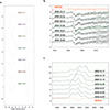 |
Fig. A.1. Time series Stokes-I spectra of RSP 348 (photometric P = 3.30 d, black lines) showing it to be a hitherto unknown SB2. a. LSD photospheric lines, b. TiO γ(0,0) band head at 7055 Å, c. Hα. Each spectrum is identified with the UT date. The red spectrum in panels b and c is the single star RSP 542 (Teff≈4000 K) for comparison. Spectra are shifted in intensity for better visibility. |
Figure A.1c reveals both components with strong Hα emission. The primary emission (peak intensity of 3.45 above continuum) is almost twice as strong as that of the secondary (peak intensity of 2.07) and shows a pronounced central self reversal indicative of a very active dMe chromosphere (e.g., Houdebine & Stempels Houdebine & Stempels (1997)). The self-reversal depth in component a is 0.41 Å (the secondary emission profile remains blended and is not measurable) while the equivalent widths are −2.35 Å and −1.00 Å for a and b, respectively. The line widths at continuum level are comparable (∼1.5 Å for both components) and are significantly larger than the absorption profile width of the comparison dM0 RSP 542 (∼1.0 Å). The respective Hα FWHM are 1.3 Å and 1.1 Å for a and b, respectively, and allow an estimate of the absolute magnitude based on the Wilson-Bappu like relation as defined in Houdebine & Stempels (Houdebine & Stempels 1997). It gives MV(a)≈10.1 mag and MV(b)≈12.2 mag, or M3 and M5 according to “standard” tables, in good agreement with the TiO-based effective temperatures.
Appendix B: Additional figures
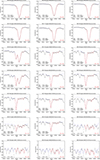 |
Fig. B.1. TurboMPfit of the lithium region (lines are the fit, dots are the observations). Fixed parameters were Teff, log g, ξt, and v sin i. Free parameters were A(Li), its isotope ratio, [Fe/H], a global Gaussian line broadening, and the continuum level. A total of 44 pixels were fitted (indicated by the red line). |
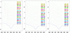 |
Fig. B.2. Ca II IRT line profiles. From left to right: IRT-1 (8498 Å), IRT-2 (8542 Å), and IRT-3 (8662 Å). Targets are arranged with increasing rotation period from bottom to top; each spectrum is consecutively shifted in intensity by 0.1 for better visibility. Targets are identified on the right side of each plot. The x-axis is wavelength in Ångstroem. |
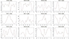 |
Fig. B.3. Longitudinal magnetic field measurements in Gauss vs. rotational phase. Shown are the data (dots with error bars) and a bicubic spline as a line to guide the eye. Each panel is for a particular target identified in the panel header (the sequence follows Table 1). Targets with data from more than one observing season are shown in separate panels with the year indicated in the header. |
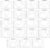 |
Fig. B.3. Continued. |
Appendix C: Additional tables
Target sample and observational phase coverage.
Observing log of individual spectra.
All Tables
All Figures
|
Fig. 1. Temperature distributions for the Hyades in our sample. a. Versus rotation period. The target in the lower right corner is the cool M dwarf binary RSP 348 (not included in the other panels). b. Versus radius as obtained from the Gaia DR3 parallax, and c. versus luminosity L. |
| In the text | |
|
Fig. 2. Comparison of the lithium 6707.8-Å region for our sample stars. We show the phase-combined spectra. The short vertical dashes indicate the wavelengths of blending lines. The bottom row of dashes shows the line list from Strassmeier & Steffen (2022), the middle row shows the strongest CaH and TiO lines from the solar umbral atlas, and the upper four dashes indicate the two 7Li and 6Li doublets, respectively. The x-axis is the wavelength in Ångstroem. |
| In the text | |
|
Fig. 3. Nineteen individual Li I 6707.8-Å line profiles of RSP 177 (Teff = 5770 K). It indicates the expected range of line-core changes over time. The black profiles are from 2020 (season S20), and the red profiles are from 2022 (season S22), according to Table C.1. The maximum line-core variability in this case is 0.8%. The x-axis is the wavelength in Ångstroem. |
| In the text | |
|
Fig. 4. Representative Stokes-V data and results for RSP 177. a. Top spectra: All available 19 LSD Stokes-V line profiles are overplotted in units of the continuum expanded by a factor 100 and shifted in intensity by 0.1 for better visibility. Bottom spectrum: Example LSD Stokes-I profile. b. Phase-resolved disk-integrated Stokes-V LSD line profiles in units of Gauss. c. Longitudinal magnetic field versus rotational phase. Indicated are the two observing seasons for this target (S22: filled dots, S20: rings). The appendix provides similar figures for the other targets (Fig. B.3). |
| In the text | |
|
Fig. 5. Lithium-activity-rotation relations. The figure compares various relations in a matrix form (columns vs. rows) of A(Li), R′IRT, and ⟨|B|⟩ (from left to right) vs. Teff, Prot, v sin i, and Ron (from top to bottom). Fits are shown for the panels for Rossby-number dependence. The line in panel l is a combined and interpolated fit from the two-piece linear fit in Eq. (6). |
| In the text | |
|
Fig. A.1. Time series Stokes-I spectra of RSP 348 (photometric P = 3.30 d, black lines) showing it to be a hitherto unknown SB2. a. LSD photospheric lines, b. TiO γ(0,0) band head at 7055 Å, c. Hα. Each spectrum is identified with the UT date. The red spectrum in panels b and c is the single star RSP 542 (Teff≈4000 K) for comparison. Spectra are shifted in intensity for better visibility. |
| In the text | |
|
Fig. B.1. TurboMPfit of the lithium region (lines are the fit, dots are the observations). Fixed parameters were Teff, log g, ξt, and v sin i. Free parameters were A(Li), its isotope ratio, [Fe/H], a global Gaussian line broadening, and the continuum level. A total of 44 pixels were fitted (indicated by the red line). |
| In the text | |
|
Fig. B.2. Ca II IRT line profiles. From left to right: IRT-1 (8498 Å), IRT-2 (8542 Å), and IRT-3 (8662 Å). Targets are arranged with increasing rotation period from bottom to top; each spectrum is consecutively shifted in intensity by 0.1 for better visibility. Targets are identified on the right side of each plot. The x-axis is wavelength in Ångstroem. |
| In the text | |
|
Fig. B.3. Longitudinal magnetic field measurements in Gauss vs. rotational phase. Shown are the data (dots with error bars) and a bicubic spline as a line to guide the eye. Each panel is for a particular target identified in the panel header (the sequence follows Table 1). Targets with data from more than one observing season are shown in separate panels with the year indicated in the header. |
| In the text | |
|
Fig. B.3. Continued. |
| In the text | |
Current usage metrics show cumulative count of Article Views (full-text article views including HTML views, PDF and ePub downloads, according to the available data) and Abstracts Views on Vision4Press platform.
Data correspond to usage on the plateform after 2015. The current usage metrics is available 48-96 hours after online publication and is updated daily on week days.
Initial download of the metrics may take a while.