| Issue |
A&A
Volume 704, December 2025
|
|
|---|---|---|
| Article Number | A78 | |
| Number of page(s) | 14 | |
| Section | Planets, planetary systems, and small bodies | |
| DOI | https://doi.org/10.1051/0004-6361/202557059 | |
| Published online | 03 December 2025 | |
Eccentric disks as a gateway to giant planet outward migration
1
Dipartimento di Fisica, Università degli Studi di Milano,
Via Celoria 16,
Milano
20133,
Italy
2
Institute of Astronomy, University of Cambridge,
Madingley Road,
Cambridge
CB3 0HA,
UK
3
School of Physics and Astronomy, University of Leeds,
Leeds
LS2 9JT,
UK
★ Corresponding author: This email address is being protected from spambots. You need JavaScript enabled to view it.
Received:
1
September
2025
Accepted:
19
September
2025
Abstract
Context. Recent studies on the planet-dominated regime of type II migration have demonstrated the presence of a correlation between the direction of massive planet migration and the parameter K that describes the depth of the gap opened by the planet. Indeed, it has been reported that high (low) values for the K parameter correspond to an outward (inward) migration.
Aims. In this paper, we aim to understand the mechanism driving inward and outward migration and why these mechanisms are correlated with the gap depth.
Methods. We performed a suite of 2D, live-planet, long-term simulations of massive planets migrating in disks with the hydro-code FARGO3D. We focused on a range of planet masses (1–13 mJ) and disk aspect ratios (from 0.03 to 0.1). We analyzed the evolution of orbital elements and gap structure. We also studied the torque contributions from outer Lindblad resonances to investigate their role in the migration outcome.
Results. We find that while all planets initially migrate inward, those with high enough K values eventually enter a phase in which the torque reverses sign and migration turns outward, until the point where it stalls. This behavior is associated with eccentricity growth in the outer disk and changes in the gap structure. We identified the surface density ratio at the 1:2 and 1:3 outer Lindblad resonances as a key output diagnostic that are correlated with the migration direction. In general, this ratio regulates the migration for all the cases where the massive planet remains in an almost circular orbit and the outer gap region exhibits moderate eccentricity. This characteristic sequence of inward-reversal-outward-stalling can occur for a variety of K values. Thus, further work is required to identify the simulation input parameters that determine the onset of this sequence.
Conclusions. Our results suggest that outward migration in the planet-dominated regime is primarily governed by the relative importance of the 1:2 and 1:3 resonances. Therefore, the gap profiles play a crucial role in determining the direction of migration.
Key words: planets and satellites: dynamical evolution and stability / planets and satellites: gaseous planets / protoplanetary disks / planet-disk interactions
© The Authors 2025
 Open Access article, published by EDP Sciences, under the terms of the Creative Commons Attribution License (https://creativecommons.org/licenses/by/4.0), which permits unrestricted use, distribution, and reproduction in any medium, provided the original work is properly cited.
This article is published in open access under the Subscribe to Open model. This email address is being protected from spambots. You need JavaScript enabled to view it. to support open access publication.
1 Introduction
Once they are formed in protoplanetary disks, planets enter into a gravitational interaction with the surrounding gas by exchanging angular momentum and orbital energy (e.g., Lin et al. 1993; Goldreich & Tremaine 1979, 1980; also see recent reviews by Papaloizou & Terquem 2006; Kley & Nelson 2012; Baruteau et al. 2014; Papaloizou 2021; Paardekooper et al. 2022). This planet-disk interaction alters the disk structures by forming, for example, spirals and gaps (e.g., Papaloizou & Lin 1984; Hourigan & Ward 1984; Kley & Nelson 2012). It also determines the evolution of the planet orbital parameters (e.g., Ward 1997). Since it modifies the planet semimajor axis and eccentricity, disk-planet interaction is therefore a key process shaping the architecture of planetary systems (e.g., Ida & Lin 2008; Mordasini 2018). Understanding the physical mechanisms that govern the direction and rate of this migration is thus essential to explain the observed distribution of exoplanets and to connect planet formation models with observations of young disks (e.g., Andrews et al. 2018; Nielsen et al. 2019; Long et al. 2018).
Depending on the planet’s mass and the disk properties, migration is typically divided into two regimes (Artymowicz 1993; Ward 1998; Kley & Nelson 2012): type I migration for low-mass, embedded planets and type II migration for massive planets that open deep gaps (e.g., Ward 1997, 1986; Lin et al. 1993; Syer & Clarke 1995; Ivanov et al. 1999). According to the classical picture, once the planet opens a gap and enters the type II migration regime, no disk material can cross the planetary gap (e.g., Papaloizou & Lin 1984; Lin et al. 1993; Ida & Lin 2008; Bitsch et al. 2013). As a consequence, if the local disk is more massive than the planet (i.e., the disk-dominated regime) the planet is locked to the viscous evolution of the disk and behaves as a gas particle; otherwise, when the planet becomes more massive than the local disk (i.e., the planet-dominated regime), its inertia is so high that it significantly slows down the migration (Syer & Clarke 1995 and Ivanov et al. 1999). These two regimes of type II migration are typically identified via the disk-to-planet mass ratio parameter, (where Σ(rp) is the disk density at the planet location and mp is the planet mass), expressed as
![Mathematical equation: $\[B=\frac{4 \pi \Sigma\left(r_{\mathrm{p}}\right) r_{\mathrm{p}}^2}{m_{\mathrm{p}}}.\]$](/articles/aa/full_html/2025/12/aa57059-25/aa57059-25-eq1.png) (1)
(1)
However, this classic view of type II migration has been challenged by recent numerical simulations showing that the disk material can cross the planetary gap (Lubow & D’Angelo 2006), thereby unlocking the planet from the disk’s viscous evolution (Duffell et al. 2014; Dürmann & Kley 2015). Several studies on the disk-dominated regime of type II migration have investigated this issue (e.g., Kanagawa et al. 2018; Robert et al. 2018; Scardoni et al. 2020, 2022; Lega et al. 2021). Some suggest that planet migration is independent of the disk viscous evolution (Dürmann & Kley 2015; Kanagawa et al. 2016, 2018), while others find that the migration rate remains proportional to the disk viscous evolution (Robert et al. 2018). It has also been demonstrated that the classical type II rate is restored if the system has enough time to adjust to the presence of a migrating planet (Scardoni et al. 2020).
A critical problem related to migration is the study of the planetary gap’s properties; as the strongest torque is exerted close to the planet, the details of the gap shape strongly influence the migration outcome (Goldreich & Tremaine 1979, 1980; Goldreich & Sari 2003). Although a detailed description of the gap is not straightforward, some works have highlighted this issue. For example, Crida et al. (2006) provided an analytical formula linking the gap properties to the planet and disk parameters. Fung et al. (2014) and Fung & Chiang (2016) studied the gap density and showed that planetary gaps produced in 3D simulations are consistent with those in 2D. Kanagawa et al. (2015) studied the gap shape and provided an empirical estimate of the gap width.
In this paper, we focus on the planet-dominated regime of type II migration (low B), which recently gained popularity with the discovery that outward migration in this regime can be easily achieved in simulations (Dempsey et al. 2020, 2021; Scardoni et al. 2022). In particular, these studies have shown that the depth and width of gap opened by the planet play a key role in determining the migration behavior, finding a correlation between the direction of migration and the gap-depth parameter (Kanagawa et al. 2015), expressed as
![Mathematical equation: $\[K=\frac{q^2}{\alpha h^5},\]$](/articles/aa/full_html/2025/12/aa57059-25/aa57059-25-eq2.png) (2)
(2)
with planets migrating outward (inward) for high (low) values of K. However, so far, such a correlation has only been found empirically (Dempsey et al. 2020, 2021) and the consequences for the distribution of exoplanets explored (Scardoni et al. 2022), while we are still lacking a physical explanation for this correlation.
Building on our previous work (Scardoni et al. 2022), our long-term integrations (ranging from 300k to 600k orbits) reveal that in some cases, a given planet exhibits a sequence of evolutionary phases: inward migration, torque reversal, outward migration, and stalling. In Section 4, we examine this behavior in detail in the case of a 1 mJ planet with aspect ratio h = H/r = 0.05, finding that torque reversal is associated with a change in gap structure and an episode of eccentricity growth in the disk exterior to the planet. We discuss the possible origin of this behavior in terms of the planet–disk interaction at the 1:3 resonance; indeed, when the 1:3 resonance becomes dominant over the 1:2 resonance, it can significantly alter the gap structure by increasing the disk eccentricity in the outer gap areas. As a result, this can impact the direction of migration. Indeed, the interaction between the disk and the planet at the outer Lindblad resonances can cause eccentricity growth in the gap area (e.g., Artymowicz 1993; Kley & Dirksen 2006; Lubow 1991; Papaloizou 2021; Tanaka et al. 2002, 2022). In particular, the 1:2 outer Lindblad resonance (located at r ~ 1.59 rp) tends to damp the eccentricity, while the 1:3 resonance (located at r ~ 2.08 rp) tends to increase the eccentricity.
We show that the change in gap shape at torque reversal can be simply parameterized in terms of the surface density ratio at the 1:2 and 1:3 resonances. We furthermore show across all simulations that the value of this ratio, derived as the simulation output, determines whether planets migrate inward, outward, or stall.
In Section 4.3, we instead attempt to map migration outcomes on to simulation input parameters, as in Scardoni et al. (2022). We, however, find that this sequence of inward migration, torque reversal and stalling occur over a wide range of values of H/r (0.04 to 0.055 for Jupiter-mass planets). This corresponds, for the flaring law considered, to around a factor of 5 in the orbital radius. We expect planets that are located within this range of H/r at the point of entering the planet-dominated regime (B < 1) to change their orbital radii by no more than a couple of 10s of percent in the B < 1 regime. Outside this range, we find that at large radius (H/r > 0.06) migration is inwards over the duration of the experiment, while at a smaller radius (H/r < 0.036), planets migrate outward throughout the simulation.
We also examine the migration behavior of more massive planets (3 mJ and 13 mJ; see Section 5) and define the limits of validity for the proposed migration mechanism. In particular, we find that migration is regulated by the 1:2 and 1:3 density ratio only when the planet eccentricity remains moderate and disk eccentricity growth is confined near the outer gap edge. In cases of high planet eccentricity or eccentricity excitation over a broad region of the disk, different mechanisms appear to dominate the migration behavior.
This paper is organized as follows: in Section 2, we introduce our set of live-planet, long-term simulations, with the orbital parameters described in Section 3. In Section 4 and Section 5, we present the migration results for Jupiter-mass and higher-mass planets, respectively. Finally, in Section 6, we discuss implications of our findings and explore alternative criteria to predict the direction of planet migration.
2 Simulations
2.1 Simulation parameters
In addition to the set of 12 simulations already presented in Scardoni et al. (2022), for this work we used 16 additional 2D hydrodynamical simulations performed with the FARGO 3D grid code (Benítez-Llambay & Masset 2016). As in the previous work, we adopted a cylindrical reference frame (r, φ) centered on the star and considered the dimensionless units G = M* = r0 = 1, where G is the gravitational constant, M* is the star mass, and r0 is the planet’s initial location. In the adopted units, ![Mathematical equation: $\[\Omega_{\mathrm{k}}^{-1}\left(r_{0}\right)=1\]$](/articles/aa/full_html/2025/12/aa57059-25/aa57059-25-eq3.png) , which means that one orbit at the initial planet location, r0, is completed in t = 2π. All the new simulations were run for at least 10tν,0 to ensure they reached the condition
, which means that one orbit at the initial planet location, r0, is completed in t = 2π. All the new simulations were run for at least 10tν,0 to ensure they reached the condition ![Mathematical equation: $\[\left|\dot{M}(r)-\dot{M}\left(r_{\text {in }}\right)\right| / \dot{M}\left(r_{\text {in }}\right) \leq 10 \%\]$](/articles/aa/full_html/2025/12/aa57059-25/aa57059-25-eq4.png) at least until r = 2.5 ap. Here, ap is the planet’s semimajor axis, tν,0 is the viscous timescale at the initial planet radius, and rin is the inner disk radius.
at least until r = 2.5 ap. Here, ap is the planet’s semimajor axis, tν,0 is the viscous timescale at the initial planet radius, and rin is the inner disk radius.
The new simulation setup is the same as the one used in Scardoni et al. (2022)1. Thus, we considered Nr = 430 logarithmically spaced cells in the radial direction ranging from rin = 0.2 to rout = 15; in the azimuthal direction (from 0 to 2π), we took Nφ = 580 linearly spaced cells. We assumed that the disk is locally isothermal, with a disk aspect ratio defined as
![Mathematical equation: $\[h=H / r=h_0 r^f,\]$](/articles/aa/full_html/2025/12/aa57059-25/aa57059-25-eq5.png) (3)
(3)
where f = 0.215 is the flaring index and h0 is the aspect ratio at the initial planet location. The viscosity was parameterized using the α prescription of Shakura & Sunyaev (1973), which is ν = αcsH, with α varying with the radius as follows
![Mathematical equation: $\[\alpha=\alpha_0 r^a,\]$](/articles/aa/full_html/2025/12/aa57059-25/aa57059-25-eq6.png) (4)
(4)
with α0 = 0.001 and a = −0.63 for all the simulations.
In the previous work, we considered three different planet masses (mp = 1 mJup, mp = 3 mJup, mp = 13 mJup). In the present work, we performed additional simulations with mp = 1 mJup and mp = 3 mJup (where mJup is the mass of Jupiter).
As in Scardoni et al. (2022), we chose the initial disk surface density at the planet location, Σ0, so that we would have B0 = 0.15 for the “massive” disk simulations and B0 = 0.046 for the “light” disk simulations (see the next section for the initial density profiles)2. We note that we only considered values of B0 < 1 because in this work, we are interested in the planet-dominated regime of type II migration. Apart from mp, h0, and Σ0, all the other parameters were kept fixed between all the simulations (which are summarized in Table 1).
2.2 Initial and boundary conditions
The initial density profile is defined as
![Mathematical equation: $\[\Sigma(r)=\Sigma_0 r^{-0.3} \cdot \mathrm{e}^{(-r / 5)^{1.7}},\]$](/articles/aa/full_html/2025/12/aa57059-25/aa57059-25-eq7.png) (5)
(5)
The disk is initially smooth and the planet mass is gradually inserted in the simulation at R0 = 1 by progressively increasing its mass during the first 50 orbits; the planet is then released and allowed to evolve under the planet–disk torques at 50 orbits, when it has reached its full mass.
To minimize any effect from the outer boundary, we set both the velocity and the gas density to zero at rout; thus, no material could enter the simulation (i.e., with a closed boundary condition). However, since the simulations were run for t ≪ tν(rout), the effect of the outer boundary condition is negligible. At the inner boundary, instead, the material velocity is chosen to match the viscous velocity as in Scardoni et al. (2020, 2022) and Dempsey et al. (2020, 2021) (i.e., the viscous boundary condition) to ensure that the torque supplied at the inner boundary is equal to the rate of angular momentum advected by accretion (i.e., the total disk angular momentum is not modified). To prevent propagation to the inner disk of spurious waves generated by boundary effects, we employed the wave damping method from de Val-Borro et al. (2006) for the radial velocity3.
3 Orbital parameters
Figure 1 shows the orbital parameters as a function of the evolutionary time (defined as the ratio between the physical time and the viscous timescale, t/tν,0) for our entire set of simulations up to 10 tν,04. The left panels show the light disk simulations (B = 0.046), while the right panels show the massive disk simulations (B = 0.15). We stress that these simulations were evolved for unusually long timescales (from 300k to 600k orbits), enabling us to capture the long-term dynamical behavior of the system, as described below; indeed, the value of the viscous timescale at the initial planet location, tν,0, ranges from ~1.16 · 105 orbits (for h = 0.03) to ~250 · 103 (for h = 0.065).
By analyzing the evolution of the semimajor axis, shown in the upper panels of Figure 1, the simulations reveal a variety of behaviors for planet migration, with planets migrating inward, outward, stalling, or changing the direction of migration during their evolution. The semimajor axis evolution appears slower in the light disk case (left panel) with respect to the massive disk case (right panel), with the evolution time scaling inversely with the disk mass; this behavior is consistent with what expected for planet-dominated type II migration, where the migration rate is slower for lower values of the disk-to-planet mass ratio B, since the torques per unit disk mass become independent of disk mass. Overall, outward migration is favored by higher mass planets and lower aspect ratio values.
The lower panels of Figure 1 show the evolution of the planet eccentricity for all the simulations. From these plots, we can notice that 1 mJup planets never develop an eccentricity higher than 0.05. In addition, 3 mJup planets have eccentricities in the range ~0.05–0.13, while 13 mJup planets instead develop to eccentricities larger than 0.2 both in the light and in the massive disk case.
Simulation parameters.
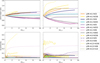 |
Fig. 1 Semimajor axis (upper panels) and eccentricity (lower panels) as a function of the evolutionary time. The left panels show the light disk simulations, the right panels show the massive disk simulations. As indicated in the legend, the solid/dashed/dotted lines show the orbital parameters for simulations with 1 mJup/3 mJup/13 mJup planets. The different colors correspond to different disk aspect ratios. |
4 Migration properties of Jupiter-mass-like planets
Initially, we focused on Jupiter-mass planets because they offer a clean benchmark to study planet migration, thanks to the low eccentricity developed by the planets during the evolution of the system. In this section, we focus on the following aspects: (1) the cause of outward migration; (2) how we can interpret the migration tracks obtained from the simulations; and (3) whether we can predict the direction of migration based on the disk and planet properties.
4.1 The role of the disk structure and eccentricity in outward planet migration
In this section, we analyze the disk structure during the evolution of the system, with the goal of understanding how the disk properties influence the direction of migration of the planet. For this purpose, we selected the simulation M-m1-h05 for our case study. We can see that the planet initially migrates inward, then reverses its direction of migration just before 2 tν,0, and, finally, end up stalling (from ~4 tν,0).
The disk evolution is illustrated in Figure 2. Here, the azimuthally averaged disk density, normalized by Σ0 = Σ(r = 1, t = 0), and eccentricity are shown in the left and right panels, respectively, as a function of radius (x-axis) and time (y-axis). The white line shows in both plots the planet migration track. From t = 0 to t ≲ 1.7 tν,0 the planet migrates inward. In this period of time, the disk density initially adjusts to the presence of the planet by creating the gap (in the very first part of the evolution) and redistributes the gas through viscosity, while the eccentricity is below 0.1 throughout the disk. Between 1.7 tν,0 ≲ t ≲ 3.8 tν,0 the planet migrates outward; meanwhile the outer gap region becomes eccentric and the amount of material passing through the gap increases, causing the inner disk region to become denser.
The increase in the outer disk eccentricity suggests the presence of a resonant interaction between the disk and the perturber (i.e., the planet). Therefore, we examined the disk density profiles close to t ~ 1.7 tν,0 in detail, where the planet changes its direction of migration. Our goal here is to understand whether a resonant interaction is occurring and whether the eccentricity increase is a cause or a consequence of the planet outward migration.
The left panel of Figure 3 illustrates the migration track for the selected simulation M-m1-h05, with an inset zooming in on the time interval around the moment when the planet changes its direction of migration, which is marked by the green dot. We also highlight some timesteps during inward migration (yellow and blue dots) and outward migration (pink and gray dots), selected just before and after the change in migration direction. The middle-left panel displays the disk density profiles corresponding to each of these timesteps, with the line colors matching those of the time markers in the left panel. From the density profiles, we can notice that as the planet switches from inward to outward migration, the density of the inner disk increases (as already observed in Figure 2), the depth of the gap decreases (coherent with the fact that there is more gas flow through the gap), and the outer gap density decreases (consistent with the outer gap area becoming eccentric). The middle-right panel shows the planet and disk eccentricity, computed through the angular momentum deficit (AMD); namely, this is the difference between the disk element angular momentum and that of an equivalent disk element on circular orbits (for a detailed computation see, e.g., Ragusa et al. 2018). We notice that both the planet and the disk eccentricity increase just before the change in sign of the direction of migration (the colored lines show the selected snapshots). From this plot, we can notice that the eccentricity starts increasing before the planet changes its direction of migration, suggesting that the change in the migration direction might be a consequence (and not a cause) of the eccentricity increase. The rapid increase in eccentricity, as previously noted, suggests the presence of a resonant interaction. Eccentricity growth at the outer gap edge can occur when the outer 1:3 Lindblad resonance becomes dominant over the outer 1:2 Lindblad resonance (see, e.g., Papaloizou et al. 2001; Goldreich & Sari 2003; Tanaka et al. 2002). Furthermore, the simultaneous increase of the AMD of both the disk and the planet cannot be the result of a secular interaction; therefore, this points to the importance of resonances at this evolutionary stage. We plot in the right panel of Figure 3 the ratio between the disk density at the 1:2 resonance Σ1:2 and that at the 1:3 resonance Σ1:3 (similar to Tanaka et al. 2022). As we can see in this plot, while the planet migrates inward, the density ratio at the two resonances is high, Σ1:2/Σ1:3 ~ 0.75, and it starts to decrease just before the change in the migration direction. Finally, Σ1:2/Σ1:3 remains low for all the outward migration phases, and it increases again when the planet stalls. We verified that the other simulations also show a similar behavior (see Appendix A)
In Figure 4, we show Σ1:2/Σ1:3 on the x-axis, while on the y-axis, we show the portion of the normalized torque responsible for the change in the semimajor axis,
![Mathematical equation: $\[\Delta T^*=\frac{J_{\mathrm{p}}}{2} \cdot \frac{\dot{a}_{\mathrm{p}}}{a_{\mathrm{p}}},\]$](/articles/aa/full_html/2025/12/aa57059-25/aa57059-25-eq8.png) (6)
(6)
where ![Mathematical equation: $\[J_{\mathrm{p}}=m_{\mathrm{p}} \sqrt{G M_{*} a_{p}(1-e_{\mathrm{p}}^{2})}\]$](/articles/aa/full_html/2025/12/aa57059-25/aa57059-25-eq9.png) is the planet angular momentum5. The colored lines correspond to the various simulations, as indicated in the legend (their colors matching those given in Figure 1). The initial and final states of each run (averaged over 30 000 orbits) are marked by a colored circle and square, respectively. Each line traces the evolution of the torque as a function of the density at the 1:2 and 1:3 resonances. The inset illustrates the typical trajectory in this plane (shown for our reference simulation M-m1-h05): the runs usually begin with negative torque and high Σ1:2/Σ1:3 > 0.8, then move toward the upper-left region of the plot (corresponding to low Σ1:2/Σ1:3 < 0.5 and positive torque) and eventually approach the zero-torque condition at intermediate values Σ1:2/Σ1:3 ~ 0.6. Not all simulations complete this loop: some remain at negative torque and high Σ1:2/Σ1:3, while others halt their evolution at positive torque and low Σ1:2/Σ1:3. The level of the evolution depends on the specific disk parameters; in this case, this is the aspect ratio. This plot therefore confirms that the 1:3 resonance (and thus the Σ1:2/Σ1:3 ratio) is key in the outward migration process.
is the planet angular momentum5. The colored lines correspond to the various simulations, as indicated in the legend (their colors matching those given in Figure 1). The initial and final states of each run (averaged over 30 000 orbits) are marked by a colored circle and square, respectively. Each line traces the evolution of the torque as a function of the density at the 1:2 and 1:3 resonances. The inset illustrates the typical trajectory in this plane (shown for our reference simulation M-m1-h05): the runs usually begin with negative torque and high Σ1:2/Σ1:3 > 0.8, then move toward the upper-left region of the plot (corresponding to low Σ1:2/Σ1:3 < 0.5 and positive torque) and eventually approach the zero-torque condition at intermediate values Σ1:2/Σ1:3 ~ 0.6. Not all simulations complete this loop: some remain at negative torque and high Σ1:2/Σ1:3, while others halt their evolution at positive torque and low Σ1:2/Σ1:3. The level of the evolution depends on the specific disk parameters; in this case, this is the aspect ratio. This plot therefore confirms that the 1:3 resonance (and thus the Σ1:2/Σ1:3 ratio) is key in the outward migration process.
As explained by Papaloizou et al. (2001), the 1:3 resonance is associated with a rapid increase in eccentricity for the planet and the edge of the outer gap by excitation of an m = 2 spiral mode. Interestingly, these authors already suggested that in cases where the outer gap eccentricity becomes high enough to alter the gap structure, a planet’s outward migration might be triggered. Indeed, in these cases, due to the different gap shape, the 1:2 resonance (favoring circular disk orbits and inward migration) becomes less important than the 1:3 resonance (favoring eccentric disk orbits and outward migration). This effect can cause the reversal of the direction of migration. The physical mechanism and intuition of the relation between the resonances and the direction of migration will be explored further in Section 4.2. In particular, they noted this effect only in cases of very massive planets, close to the brown dwarf regime; however, lower viscosity and higher integration time in our case might make the effect possible for lower mass planets. Another difference in our work compared to Papaloizou et al. (2001) is that we are dealing with an inner disk and so, the shift to outward migration is likely to be driven not only by the change in density profile exterior to the planet, but also by the factor two increase in surface density interior to the planet during the period of torque reversal. Nevertheless, we find that the simple surface density ratio proposed is a good predictor of the sign of the torque (see Figure 4). Figure 4 therefore demonstrates that the planet torque is a well-defined function of an output of the simulation (describing gap shape), but it is not useful for predicting what range of input parameters map onto each outcome. This will be explored in Section 4.3.
Finally, we investigated the impact of varying the initial and boundary conditions. We found that the initial conditions do not influence the results, whereas the boundary conditions can affect them. In particular, imposing a viscous inflow delivers material more efficiently from the outer disk to the gap region, modifying the disk structure and, consequently, the details of migration (see Appendix B for more details).
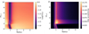 |
Fig. 2 Simulation M-m1-h05. The color maps show the azimuthal average of the disk normalized density Σ/Σ0 (left panel) and of the disk eccentricity (right panel) as a function of the disk radius (x-axis) and of evolutionary time t/tν,0 (y-axis). The white line in both plots shows the planet migration track. |
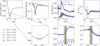 |
Fig. 3 Analysis of the migration behavior in simulation M-m1-h05. The left panel shows the semimajor axis as a function of the evolutionary time, with a zoom in the region where the planet changes its direction of migration, marked via the green dot. The other colored dots mark selected snapshots just before and after the change in migration direction. The middle-left panel shows the density profiles at the selected snapshots. The middle-right panel shows the disk (dark purple) and planet eccentricity (medium purple) evolution. The colored regions highlight the selected snapshots. The plot in the right panel illustrates the density ratio at the 1:2 and 1:3 resonances. |
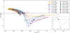 |
Fig. 4 Portion of the normalized torque responsible for the change in the semimajor axis as a function of the density ratio at the 1:2 and 1:3 resonances Σ1:2/Σ1:3. Different colors indicate different disk aspect ratios at 5 au, as indicated in the legend. Markers indicate the state of each simulation at t = 10 tν. The lines show the evolution of each simulation, whose start is shown by the circles. The inset shows the evolution track for the simulation M-m1-h05. The high (low) line opacity corresponds to the lower (higher) disk mass regimes. |
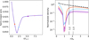 |
Fig. 5 Migration track (left panel) and density profiles (right panel). The colored dots in the left panel show some selected snapshots for inward (orange), outward (light blue), and stalling (purple and pink) phase of migration. The density profiles in the right panel are shown in colors corresponding to the dots in the left panels. |
4.2 Interpretation of inward and outward migration phases
The fact that the direction of migration is related to the Σ1:2/Σ1:3 ratio implies that the gap structure plays a primary role in determining the direction of migration. Indeed, outward migration takes place when Σ1:2/Σ1:3 drops to values ≲0.5, meaning that, in principle, there should be a limiting gap width and/or steepness which triggers outward migration. Specifically, when both the resonances are located outside the limiting gap width, the density at their location is comparable and the planet migrates inward; when the 1:2 resonance enters the limiting gap width, the density at the 1:2 resonance drops and the 1:3 resonance dominates, causing planet outward migration6. All simulations initially undergo an inward migration; then, some continue inward, while others transition to outward migration or outward migration followed by stalling. Given this understanding of migration, we can divide the migration into three phases (not all necessarily occurring for all the planets) and interpret them as follows:
Inward migration phase: the gap is relatively narrow (low K) and, thus, both the resonances are outside the gap and the Σ1:2/Σ1:3 ratio is high, meaning that the planet and disk orbits remain effectively circular. Consequently, the planet migrates inward according to regular planet-dominated type II migration. The gap profile in this migration phase for our test simulation M-m1-h05 is illustrated by the orange line in the right panel of Figure 5.
Outward migration phase: the gap is deep (high K) and wide enough to reduce the amount of disk material at the 1:2 resonance, as can be seen from the gap profile in the right panel of Figure 5 (light blue line). This means that the Σ1:2/Σ1:3 ratio becomes low and the outer gap edge becomes eccentric, altering the gap structure. As a consequence, the inner disk torque dominates over the outer disk torque (as now the outer gap is larger due to eccentricity) and the planet migrates outward.
Stalling phase. This phase usually follows an outward migration phase (however small). One possible explanation is that while the planet migrates outward, it moves closer to the outer gap edge; it is therefore possible that outward migration leads to a refilling of the 1:2 resonance. Meanwhile, the inner gap edge does not lag behind as the planet migrates outward thanks to the material passing through the gap, which is increased during outward planet migration and replenishes the inner disk. This restores the equilibrium between the inner and outer contributions to the torque and causes the stalling of the planet. This situation is illustrated by the purple and pink lines in the right panel of Figure 5, showing the gap profiles at two different times of the stalling phase. Once a system attains a situation of zero torque, then the planet is stationary thereafter. This means that the disk is not experiencing a time-dependent torque from the planet or (to put it another way) the gap shape is not having to continuously readjust to the changing location of the planet and the change in local h. This is considered to be a “stable point” of the system and subsequent evolution drains down the disk surface density (as can be seen by comparing the purple and pink gap profiles), but it does not affect the normalized torque.
Although this interpretation can explain these three different migration phases, it remains to be understood why the torques always tend to arrange a situation of zero effective torque on the planet.
4.3 Identifying an ordering parameter for the sign of planet migration
In Scardoni et al. (2022), we suggested that the turning point for the torque sign, previously found in fixed-planet simulations by Dempsey et al. (2020) and Dempsey et al. (2021), is also present in live-planet simulations and is correlated with the gap depth parameter K (Equation (2)). The limited number of simulations used in that work, however, inevitably required further investigation to confirm the presence of a “universal” limiting gap-shape parameter, Klim, corresponding to zero torque (and thus the existence of a stalling radius). We now understand that the direction of migration is set by the relative importance of the 1:3 resonance with respect to the 1:2 resonance: the 1:3 governs eccentricity excitation at the outer gap edge, leading to depletion of material in the outer gap region and outward migration. Meanwhile, the 1:2 resonance promotes circular orbits for the disk material and, therefore, these resonances do not lead to any change in the outer gap structure. Consequently, the ratio Σ1:2/Σ1:3 is correlated with the direction of migration, with high (low) values favoring inward (outward) migration. Our interpretation of the different migration phases (Section 4.2) suggests that the gap shape plays an important role in determining Σ1:2/Σ1:3 and, thus, the migration direction. We therefore explore whether, given the larger parameter space explored in this paper, the gap-depth parameter, K, is still a good ordering parameter.
Figure 6 shows the evolution of the portion of the torque associated to the change in the semimajor axis, for the subset of simulations with 1 mJ planets. The starting point for each simulation is shown by the dot, the final point at 10 tν,0 is shown by the marker (styles as in the previous plots); the initial and final locations of each simulation are connected via lines that are a slightly lighter (darker) in color for the light (massive) disk case.
Focusing first on the properties of the simulations at 10 tν,0, shown by the square markers, we can confirm that K roughly sorts the simulations into those with steady inward migration and steady outward migration. However, contrary to what was expected from Scardoni et al. (2022), there is no unique location of zero torque (i.e., there is not a single limiting value Klim). Instead, there is a range of K (~103.3−103.9) values over which the system settles to zero torque, making relatively small adjustments to its orbital radius in the process. Outside this range of K, the evolution is monotonically directed inward or outward over the duration of the simulation. The fact that parameter K cannot capture the zero torque location properly is likely because K is controls the gap depth, not the width (which is what causes the reduction of material at the 1:2 resonance). However, since deeper gaps are usually also wider, K is still a relatively good sorting parameter when we consider simulations far from the transition to zero torque. We refer to Section 6.3 for more details on the sorting criterion.
We can further notice that, in general, the light and massive versions of each system follow the same torque-K evolution. The light disk cases are less evolved (likely because the lower B value makes planet migration slower); therefore, they “lag behind” the massive cases. This suggests that the direction of migration is not influenced by the disk-to-planet mass ratio and that this phenomenon is not dependent on a specific history of disk–planet eccentricity exchange. Furthermore, the fact that this happens at different evolutionary times means that the phenomenon is independent of the disk evolution. All of these findings point to the likelihood of a local effect and, thus, a local criterion that determines the direction of migration. On the other hand, however, the disk-to-planet mass ratio is still important in determining the distribution of planets after disk dispersal; this is still influenced by the B parameter, since it is determined by the combination of the migration speed and the disk evolution timescale (as discussed in Scardoni et al. 2022). In Section 5, we explore how well the ordering parameter works as a function of q (i.e., whether the regimes described for K for 1 mJ planets work also for higher mass planets).
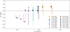 |
Fig. 6 Portion of the normalized torque responsible for the change in the semimajor axis as a function of the gap-shape parameter, K. Different colors indicate different disk aspect ratios at 5 au, as indicated in the legend. Markers indicate the state of each simulation at t = 10 tν,0. The lines show the evolution of each simulation. The high (low) line opacity corresponds to the lower (higher) disk mass regimes. |
5 Migration of higher mass planets
After studying the details of migration for Jupiter-mass-like planets, we extended our analysis to higher-mass planets to explore how the planet mass influences migration. Higher mass planets carve deeper and larger gaps in the disk and, as a result, we expect them to be more prone to outward migration.
In Figure 7, we plot the normalized torque as a function of the gap depth parameter K (left panel) and the Σ1:2/Σ1:3 ratio (right panel) for the simulations with higher mass ratio planets. The plot in the left panel confirms that also in the case of higher mass planets, the light and massive version of each simulation have the same evolution (but different evolutionary timescales) in this plane. The right panel, instead, shows some differences with the corresponding plot for Jupiter-mass planets (Figure 4), In particular, three simulations (M-m3-h05, L-m13-h10, and M-m13-h10 get to the zero torque conditions for values of Σ1:2/Σ1:3 relatively low, which usually corresponds to outward migration.
We noticed that the disks hosting 13 mJ planets become highly eccentric, with high eccentricity (up to ~0.5) extending up to r = 5 and also involving some part of the inner disk7. Furthermore, Figure 1 shows that also the planet eccentricity is higher for higher mass planets. Given the different disk structure and planet eccentricity, we believe that these high-mass planets are likely entering a different migration regime, as the migration picture emerging from the previous section only applies to systems where the planet remains on a relatively circular orbit and only the outer gap region becomes eccentric. In particular, since the migration regime described in Section 4 is only valid for quasi-circular planets migrating in disks that only grow in eccentricity close to the outer gap, we need to exclude the following simulations from our analysis of the inward and outward migration and stalling behavior: L-m3-h036, M-m3-h05, L-m13-h036, M-m13-h036, L-m13-h06, M-m13-h06, L-m13-h10, M-m13-h108.
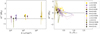
In Figure 8, we show the normalized torque associated with the change in the semimajor axis (at 3 tν,0 and 10 tν,0 in the left and right panel, respectively) as a function of the gap shape parameter for the entire set of simulations. The systems entering a different migration regime are shown with translucent markers. This plot confirms that planets in systems characterized by high (low) K values migrate outward (inward), even when we consider higher mass planets, provided that we only consider the systems migrating according to the migration regime described in Section 4 (i.e., circular planet orbits and moderate disk eccentricity). From Figure 6 and the left panel of Figure 7 we understand that each system is undergoing its own little loop in ![Mathematical equation: $\[\Delta T^{*} /\left|\dot{M} l_{\mathrm{p}}\right|\]$](/articles/aa/full_html/2025/12/aa57059-25/aa57059-25-eq10.png) versus K space on its own timescale; therefore the big scatter in torques at a given K value in the range ~2000–10 000 in Figure 8 (only considering simulations in the circular planet, eccentric outer gap migration regime) reflects different timescales in performing the same loop.
versus K space on its own timescale; therefore the big scatter in torques at a given K value in the range ~2000–10 000 in Figure 8 (only considering simulations in the circular planet, eccentric outer gap migration regime) reflects different timescales in performing the same loop.
6 Discussion
6.1 Disk and planet parameters for outward migration
Although it is not the ideal parameter for sorting the inward and outward migration around the point where the torques switch their sign, K is still a good sorting parameter for inward and outward migration far from ![Mathematical equation: $\[\Delta T /\left|\dot{M} l_{\mathrm{p}}\right|=0\]$](/articles/aa/full_html/2025/12/aa57059-25/aa57059-25-eq11.png) . In Figure 9, we therefore explore the K map as a function of the local disk aspect ratio, h (y axis), and planet mass, mp (x axis) for α = 10−3 (as that considered in our set of simulations). The brown-yellow area indicates the combination of h, α, mp that can produce inward migration; the teal area shows the combination of parameters that is expected to correspond to outward migration. The area between log(K) = 3.3 and log(K) = 4 (indicated by gray lines) is the region where there is a significant scatter in the values of the normalized torque. As expected, higher mass planets are more prone to outward migration with respect to the lower mass planets9. Nonetheless, these plots show that reasonable disk parameters can produce outward migration for 1 mJup. This means that outward migration is not hard to obtain in this mass regime.
. In Figure 9, we therefore explore the K map as a function of the local disk aspect ratio, h (y axis), and planet mass, mp (x axis) for α = 10−3 (as that considered in our set of simulations). The brown-yellow area indicates the combination of h, α, mp that can produce inward migration; the teal area shows the combination of parameters that is expected to correspond to outward migration. The area between log(K) = 3.3 and log(K) = 4 (indicated by gray lines) is the region where there is a significant scatter in the values of the normalized torque. As expected, higher mass planets are more prone to outward migration with respect to the lower mass planets9. Nonetheless, these plots show that reasonable disk parameters can produce outward migration for 1 mJup. This means that outward migration is not hard to obtain in this mass regime.
6.2 Stalling radius and comparison with the toy model
In our approximate model, based on the idea that the normalised torque is correlated with K, the stalling radius is defined as (see also Scardoni et al. 2022):
![Mathematical equation: $\[r_{\lim }=\left(\frac{q^2}{K_{\lim } \alpha_0 h_0^5}\right)^{1 /(a+5 f)}.\]$](/articles/aa/full_html/2025/12/aa57059-25/aa57059-25-eq12.png) (7)
(7)
However, given the uncertainties in Klim, predicting the exact stalling radius remains challenging. In Figure 10, we show the evolution of a subset of simulations with Jupiter-mass planets in physical units. To convert from code units to physical units, we assumed a disk with h = 0.05 at 5 au (corresponding to simulation M-m1-h05), which translates to h ~ 0.035 at 1 au. The simulation tracks are shown as solid lines for the light and massive disk cases in the left and right panels, respectively. From this plot, we note that in the selected disk model, the typical stalling radius stalls between 3–5 au (see the cyan and magenta lines). If we consider our range of h = 0.03–0.065 at 5 au (corresponding to ~0.02–0.05 at 1 au), the stalling radius ranges from 0.5 au to 50 au; this underlines that the stalling radius is quite sensitive to the aspect ratio (indeed, the gap properties are sensitive to h).
Furthermore, we indicate with dashed lines the predicted evolution according to the toy model of Scardoni et al. (2022) (with W = 1 and Klim = 3500), which provides an analytical estimate of the migration track based solely on the gap-shape parameter. While the toy model does not capture the full complexity of gap eccentricity and long-term disk evolution, it nonetheless reproduces the qualitative behavior observed in our simulations, including the occurrence of outward migration and stalling at radii of a few au. This highlights the need for a precise gap profile model in order to be able to predict the migration precisely. We notice that the toy model captures the migration tracks of outward-migrating planets quite well; whereas it tends to predict slower migration than observed in the simulations for inward-migrating planets. This discrepancy is likely due to a transient phase in which inward-migrating planets move faster than the velocity prescribed by type II migration (see Scardoni et al. 2020). At later times, the migration rate tends to slow to values more consistent with the prediction (this can be seen clearly from the gray lines, which evolved for longer than the pink and magenta cases). Nonetheless, the initial fast transient is significant enough to make the prescription for inwardly migrating planets inaccurate.
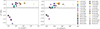 |
Fig. 8 Portion of the normalized torque responsible for the change in the semimajor axis as a function of the gap-shape parameter, K. In the left panel, the plot shows the distribution of the simulations at t = 3 tν,0, while the right panel shows the distribution at t = 10 tν,0. The marker shape indicates the planet mass: 1 mJup (squares), 3 mJup (circles), and 13 mJup (diamonds). The colors indicate the disk aspect ratio at 5 au. Dashed markers indicate the massive disk simulations. The translucent markers indicate the systems entering a different migration regime with respect to that studied in this paper. |
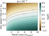 |
Fig. 9 Gap-shape parameter, K, map as a function of the local disk aspect ratio (y-axis) and planet mass (x-axis). Some reference values for K are highlighted via the gray contours (the “stalling region” is within the interval log(K) = [3.3, 4.1]). The brown-yellow area indicates the combination of h, α, mp that is expected to generate inward migration; the teal area shows the combination of parameters that is expected to correspond to outward migration. |
6.3 Alternative criteria for sorting the simulations according to their direction of migration
So far, we have discussed the ![Mathematical equation: $\[\Delta T /\left|\dot{M} l_{\mathrm{p}}\right|-K\]$](/articles/aa/full_html/2025/12/aa57059-25/aa57059-25-eq13.png) relation, noticing that the gap-depth parameter is a relatively good parameter for describing and predicting the direction of migration. As noticed in Section 4.2, however, the direction of migration is actually driven by the relative importance of the 1:2 and 1:3 outer resonances; therefore, the ideal parameter to predict the direction of migration would be a gap width parameter that would allow us to determine whether the 1:2 resonance is located inside or outside the gap. However, obtaining such a parameter would require precise knowledge of the gap shape. The closest parameter available at the moment is the gap-width parameter, K′ = q2/(αh3), derived by Kanagawa et al. (2015). We tested the ability of K′ to predict the direction of migration, as detailed in Figure 11. We find that although the migration behavior can be efficiently predicted for high and low values of K′, it cannot precisely predict the zero torque (or the direction of migration turning point). This means that the K′ parameter is probably not precise enough to describe the gap-width for this particular problem.
relation, noticing that the gap-depth parameter is a relatively good parameter for describing and predicting the direction of migration. As noticed in Section 4.2, however, the direction of migration is actually driven by the relative importance of the 1:2 and 1:3 outer resonances; therefore, the ideal parameter to predict the direction of migration would be a gap width parameter that would allow us to determine whether the 1:2 resonance is located inside or outside the gap. However, obtaining such a parameter would require precise knowledge of the gap shape. The closest parameter available at the moment is the gap-width parameter, K′ = q2/(αh3), derived by Kanagawa et al. (2015). We tested the ability of K′ to predict the direction of migration, as detailed in Figure 11. We find that although the migration behavior can be efficiently predicted for high and low values of K′, it cannot precisely predict the zero torque (or the direction of migration turning point). This means that the K′ parameter is probably not precise enough to describe the gap-width for this particular problem.
For the moment, we believe that the best available parameter to predict the direction of migration remains K, given the lower relative uncertainty at the turning point for the direction of migration. However, we caution that this parameter is not able to capture the details of migration close to the turning point. We believe that a precise prediction of the direction of migration necessarily requires a deep investigation of the gap shape.
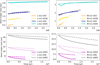 |
Fig. 10 Evolution of Jupiter-mass planets in physical units for light (left) and massive (right) disks. Solid lines show simulation tracks, while dashed lines indicate predictions from the toy model of Scardoni et al. (2022) (W = 1, Klim = 3500). |
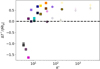 |
Fig. 11 Normalized torque as a function of the gap-width parameter K′ = q2/αh3. |
7 Conclusions
In this work, we investigated the migration of massive planets in the planet-dominated regime of type II migration, focusing on the transition between inward and outward migration. Building upon the torque framework introduced in Scardoni et al. (2022), we have run a suite of simulations that explore a wide range of planet masses and aspect ratios, while keeping the α viscosity parameter fixed. Our main findings can be summarized as follows:
A critical insight emerging from our analysis is the key role of the 1:2 and 1:3 outer Lindblad resonances in determining the migration direction (Sections 4.1 and 4.2). The relative positioning of these resonances with respect to the outer gap edge strongly influences their contribution to the torque acting on the planet and, therefore, the overall torque balance; as well as the migration outcome as a result. Specifically, at the beginning of the simulations both resonances lie outside the gap; thus, the 1:2 resonance dominates, the disk remains circular, and the planet migrates inward. While the system evolves, in some cases, the 1:2 resonance shifts inside the gap region. Consequently, its contribution weakens, allowing the 1:3 resonance that remains in the high-density region outside the gap to dominate. When the 1:3 resonance dominates, it causes an increase in the eccentricity of the disk outer gap region and favors the gas passage through the gap. These effects significantly alter the gap structure, causing the density to increase in the inner disk and to decrease in the outer gap region, leading to outward migration. Finally, during the outward migration phase, the outer gap eccentricity tends to decrease and the gap shape tends to assess an equilibrium, causing the planet to stall;
In Section 4.3, we confirmed that the gap-depth parameter K = q2/(αh5) is a reasonably effective predictor of the migration direction, with outward migration favored for higher K (i.e., higher planet masses, lower viscosity, thinner disks), as already suggested by Scardoni et al. (2022). However, we found that while K performs well far from the torque transition region 2500 < K < 10 000, it becomes less reliable near the turning point, where the migration direction switches sign. The stalling radius (i.e., the orbital location corresponding to the zero torque condition), which depends on a critical value of K, also remains uncertain because the torque reversal and stalling can occur over a broad range of K values. We tested the gap-width parameter K′ as an alternative, but found it less effective in predicting the turning point of migration (Section 6.3). This implies that the precise location of the migration turning point remains uncertain, as simple gap parameters cannot capture the migration behavior close to the zero torque condition. Therefore, we suggest that the best parameter to predict the direction of migration would be a precise gap-width parameter, but this is not available at the moment;
Our findings suggest that outward migration is not only obtained for extreme disk conditions, but it can occur for Jupiter-mass planets in reasonable disk environments (Sections 6.1 and 6.2);
In Section 5 we extended our analysis to higher mass planets, finding that this new migration regime regulated by the 1:2 and 1:3 outer resonances is only valid for systems with near circular orbit planets and disks with relatively high eccentricity in outer gap region; in cases where the planet becomes significantly eccentric or the disk eccentricity involves large areas of the disk (including the inner disk or outer disk far away from the gap), the system enters a different regime and cannot be described by our analysis.
While the results presented in this paper provide valuable insights into the migration behavior of massive planets, several limitations and unresolved issues remain. In the following, we outline the key caveats in our current approach, as well as open questions that remain. The Σ1:2/Σ1:3 ratio remains descriptive (rather than predictive) of the direction of planet migration, while the gap-depth parameter, K, does not reliably capture migration behavior near the zero-torque condition. A precise prediction of the migration turning point requires a more accurate characterization of the gap structure. The uncertainties in torque prescriptions near the transition regime must be carefully considered when applying these results to population synthesis models or interpreting observations. Finally, we note that it remains unclear why planets in this migration regime systematically evolve toward the equilibrium condition (i.e., zero net torque).
Acknowledgements
We thank the referee for a careful reading of the manuscript and helpful comments. We thank Alessandro Morbidelli and Elena Lega for valuable discussions that significantly contributed to this study. C.E.S and G.P.R. acknowledge support from the European Union (ERC Starting Grant DiscEvol, project No. 101039651) and from Fondazione Cariplo, grant No. 2022-2017. Views and opinion expressed are, however, those of the author(s) only and do not necessarily reflect those of the European Union or European Research Council. Neither the European Union nor the granting authority can be held responsible for them. CJC has been supported by the UK Science and Technology research Council (STFC) via the consolidated grant ST/W000997/1. ER acknowledges financial support from the European Union’s Horizon Europe research and innovation programme under the Marie Skłodowska-Curie grant agreement No. 101102964 (ORBIT-D). RAB thanks the Royal Society for their support through a University Research Fellowship. This work was in part performed using the Cambridge Service for Data Driven Discovery (CSD3), part of which is operated by the University of Cambridge Research Computing on behalf of the STFC DiRAC HPC Facility (www.dirac.ac.uk). The DiRAC component of CSD3 was funded by BEIS capital funding via STFC capital grants ST/P002307/1 and ST/R002452/1, and STFC operations grant ST/R00689X/1. This work was in part performed at CINECA, with computational resources on the LEONARDO super-computer, owned by the EuroHPC Joint Undertaking and hosted by CINECA (Italy).
References
- Andrews, S. M., Huang, J., Pérez, L. M., et al. 2018, ApJ, 869, L41 [NASA ADS] [CrossRef] [Google Scholar]
- Artymowicz, P. 1993, ApJ, 419, 166 [NASA ADS] [CrossRef] [Google Scholar]
- Baruteau, C., Crida, A., Paardekooper, S. J., et al. 2014, in Protostars and Planets VI, eds. H. Beuther, R. S. Klessen, C. P. Dullemond, & T. Henning, 667 [Google Scholar]
- Benítez-Llambay, P., & Masset, F. S. 2016, ApJS, 223, 11 [Google Scholar]
- Bitsch, B., Crida, A., Morbidelli, A., Kley, W., & Dobbs-Dixon, I. 2013, A&A, 549, A124 [NASA ADS] [CrossRef] [EDP Sciences] [Google Scholar]
- Crida, A., Morbidelli, A., & Masset, F. 2006, Icarus, 181, 587 [Google Scholar]
- de Val-Borro, M., Edgar, R. G., Artymowicz, P., et al. 2006, MNRAS, 370, 529 [Google Scholar]
- Dempsey, A. M., Lee, W.-K., & Lithwick, Y. 2020, ApJ, 891, 108 [Google Scholar]
- Dempsey, A. M., Muñoz, D. J., & Lithwick, Y. 2021, arXiv e-prints [arXiv:2105.05277] [Google Scholar]
- Duffell, P. C., Haiman, Z., MacFadyen, A. I., D’Orazio, D. J., & Farris, B. D. 2014, ApJ, 792, L10 [Google Scholar]
- Dürmann, C., & Kley, W. 2015, A&A, 574, A52 [NASA ADS] [CrossRef] [EDP Sciences] [Google Scholar]
- Fung, J., & Chiang, E. 2016, ApJ, 832, 105 [NASA ADS] [CrossRef] [Google Scholar]
- Fung, J., Shi, J.-M., & Chiang, E. 2014, ApJ, 782, 88 [NASA ADS] [CrossRef] [Google Scholar]
- Goldreich, P., & Sari, R. 2003, ApJ, 585, 1024 [Google Scholar]
- Goldreich, P., & Tremaine, S. 1979, ApJ, 233, 857 [Google Scholar]
- Goldreich, P., & Tremaine, S. 1980, ApJ, 241, 425 [Google Scholar]
- Hourigan, K., & Ward, W. R. 1984, Icarus, 60, 29 [Google Scholar]
- Ida, S., & Lin, D. N. C. 2008, ApJ, 673, 487 [NASA ADS] [CrossRef] [Google Scholar]
- Ivanov, P. B., Papaloizou, J. C. B., & Polnarev, A. G. 1999, MNRAS, 307, 79 [Google Scholar]
- Kanagawa, K. D., Tanaka, H., Muto, T., Tanigawa, T., & Takeuchi, T. 2015, MNRAS, 448, 994 [NASA ADS] [CrossRef] [Google Scholar]
- Kanagawa, K. D., Muto, T., Tanaka, H., et al. 2016, PASJ, 68, 43 [NASA ADS] [Google Scholar]
- Kanagawa, K. D., Tanaka, H., & Szuszkiewicz, E. 2018, ApJ, 861, 140 [Google Scholar]
- Kley, W., & Dirksen, G. 2006, A&A, 447, 369 [NASA ADS] [CrossRef] [EDP Sciences] [Google Scholar]
- Kley, W., & Nelson, R. P. 2012, ARA&A, 50, 211 [Google Scholar]
- Lega, E., Nelson, R. P., Morbidelli, A., et al. 2021, A&A, 646, A166 [NASA ADS] [CrossRef] [EDP Sciences] [Google Scholar]
- Lin, D. N. C., Papaloizou, J. C. B., & Kley, W. 1993, ApJ, 416, 689 [Google Scholar]
- Long, F., Pinilla, P., Herczeg, G. J., et al. 2018, ApJ, 869, 17 [Google Scholar]
- Lubow, S. H. 1991, ApJ, 381, 259 [Google Scholar]
- Lubow, S. H., & D’Angelo, G. 2006, ApJ, 641, 526 [Google Scholar]
- Mordasini, C. 2018, in Handbook of Exoplanets, eds. H. J. Deeg, & J. A. Belmonte, 143 [Google Scholar]
- Nielsen, E. L., De Rosa, R. J., Macintosh, B., et al. 2019, AJ, 158, 13 [Google Scholar]
- Paardekooper, S.-J., Dong, R., Duffell, P., et al. 2022, arXiv e-prints [arXiv:2203.09595] [Google Scholar]
- Papaloizou, J. C. B. 2021, arXiv e-prints [arXiv:2107.07269] [Google Scholar]
- Papaloizou, J., & Lin, D. N. C. 1984, ApJ, 285, 818 [NASA ADS] [CrossRef] [Google Scholar]
- Papaloizou, J. C. B. & Terquem, C. 2006, Rep. Progr. Phys., 69, 119 [Google Scholar]
- Papaloizou, J. C. B., Nelson, R. P., & Masset, F. 2001, A&A, 366, 263 [NASA ADS] [CrossRef] [EDP Sciences] [Google Scholar]
- Ragusa, E., Rosotti, G., Teyssandier, J., et al. 2018, MNRAS, 474, 4460 [CrossRef] [Google Scholar]
- Robert, C. M. T., Crida, A., Lega, E., Méheut, H., & Morbidelli, A. 2018, A&A, 617, A98 [NASA ADS] [CrossRef] [EDP Sciences] [Google Scholar]
- Rosotti, G. P., Booth, R. A., Clarke, C. J., et al. 2017, MNRAS, 464, L114 [Google Scholar]
- Scardoni, C. E., Rosotti, G. P., Lodato, G., & Clarke, C. J. 2020, MNRAS, 492, 1318 [NASA ADS] [CrossRef] [Google Scholar]
- Scardoni, C. E., Clarke, C. J., Rosotti, G. P., et al. 2022, MNRAS, 514, 5478 [NASA ADS] [CrossRef] [Google Scholar]
- Shakura, N. I., & Sunyaev, R. A. 1973, in IAU Symposium, 55, X- and Gamma-Ray Astronomy, eds. H. Bradt, & R. Giacconi, 155 [Google Scholar]
- Syer, D., & Clarke, C. J. 1995, MNRAS, 277, 758 [NASA ADS] [Google Scholar]
- Tanaka, H., Takeuchi, T., & Ward, W. R. 2002, ApJ, 565, 1257 [Google Scholar]
- Tanaka, Y. A., Kanagawa, K. D., Tanaka, H., & Tanigawa, T. 2022, ApJ, 925, 95 [NASA ADS] [CrossRef] [Google Scholar]
- Ward, W. R. 1986, Icarus, 67, 164 [Google Scholar]
- Ward, W. R. 1997, Icarus, 126, 261 [Google Scholar]
- Ward, W. R. 1998, in Astronomical Society of the Pacific Conference Series, 148, Origins, eds. C. E. Woodward, J. M. Shull, & J. Thronson, Harley A., 338 [Google Scholar]
Analogously to Ragusa et al. (2018) and Rosotti et al. (2017).
For reference, if we consider a Jupiter-mass planet at the radius of Jupiter, B0 = 0.046 and B0 = 0.15 correspond (in physical units) to a local disk surface density of 1.3 g/cm2 and 4.2 g/cm2, respectively.
Over the damping timescale (![Mathematical equation: $\[\tau=\Omega_{\mathrm{k}}^{-1} / 30\]$](/articles/aa/full_html/2025/12/aa57059-25/aa57059-25-eq17.png) ), we damped vr to the azimuthal average of the initial (viscous) velocity ⟨νr,0⟩ in the region from rin to r = 0.3.
), we damped vr to the azimuthal average of the initial (viscous) velocity ⟨νr,0⟩ in the region from rin to r = 0.3.
We limited our analysis to 10 tν,0 to avoid spurious effects from the outer boundary, where the viscous timescale is ~19tν,0.
Note: the total torque acting on the planet is ![Mathematical equation: $\[\Delta T=\Delta T^{*}- J_{\mathrm{p}} e /\left(1-e^{2}\right) \cdot \dot{e}\]$](/articles/aa/full_html/2025/12/aa57059-25/aa57059-25-eq18.png)
We note, however, that at the moment there is no gap-width parameter precise enough to capture whether or not the two resonances are both outside the gap or the 1:2 resonance has shifted inside it.
Note that these behaviors have been verified but the corresponding plots are omitted for conciseness.
We verified that the high eccentricity in these simulations do no cause problematic interaction with the inner boundary by checking that the orbital area of the planet (ap (1 ± ermp)) does not get close to the inner boundary over the entire simulation run.
In principle, lower values of the α viscosity parameter tend to favor outward migration, while higher values favor inward migration. However, because we did not test different α values and the migration direction depend strongly on the gap shape, this expectation requires confirmation through further simulations.
Note: Σ1:2/Σ1:3 is initially very high for all the simulations because of the initial conditions, where the planet is not present, but it is gradually inserted over the first 50 orbits of the simulation.
For closed boundary conditions, outward radial flow occurs because the system’s material can freely adjust according to viscosity. By contrast, with a forced viscous outer boundary, the inward viscous flow is imposed, so no radial outflow is expected.
Appendix A Evolution of the 1:3 versus 1:3 resonances
In Figure A.1, the colored lines show the Σ1:2/Σ1:3 ratio as a function of the evolutionary time, t/tν,0, for all simulations with 1 Jupiter mass planets. The light gray line in each plot shows the rate of change of the planet semimajor axis, ![Mathematical equation: $\[\dot{a}_{\mathrm{p}} /\left|\max \left(\dot{a}_{\mathrm{p}}\right)\right|\]$](/articles/aa/full_html/2025/12/aa57059-25/aa57059-25-eq14.png) .
.
We notice a strong correlation between the value of Σ1:2/Σ1:3 ratio and ![Mathematical equation: $\[\dot{a}_{\mathrm{p}} /\left|\max \left(\dot{a}_{\mathrm{p}}\right)\right|\]$](/articles/aa/full_html/2025/12/aa57059-25/aa57059-25-eq15.png) : inward (outward) migration phases are associated with high (low) values for Σ1:2/Σ1:310. This suggests that the 1:3 resonance, and therefore Σ1:2/Σ1:3, is key in the outward migration process. Similar results are found for all the other simulations in this migration regime (L-m3-h036, M-m3-h036, L-m3-h05, M-m3-h05, and M-m3-h06).
: inward (outward) migration phases are associated with high (low) values for Σ1:2/Σ1:310. This suggests that the 1:3 resonance, and therefore Σ1:2/Σ1:3, is key in the outward migration process. Similar results are found for all the other simulations in this migration regime (L-m3-h036, M-m3-h036, L-m3-h05, M-m3-h05, and M-m3-h06).
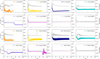 |
Fig. A.1 Ratio between the disk density at the 1:2 resonance and at the 1:3 resonance for all simulations with 1 mJup planets (colored lines), as indicated in each panel legend. The gray lines in each plot show the rate of change of the planet semimajor axis, |
![Mathematical equation: $\[\dot{a}_{\mathrm{p}} /\left|\max \left(\dot{a}_{\mathrm{p}}\right)\right|\]$](/articles/aa/full_html/2025/12/aa57059-25/aa57059-25-eq16.png)
Appendix B Varying the initial and boundary conditions
In this appendix, we check whether the initial or boundary conditions influence the outcome of migration and the stalling radius. For this purpose, we take as reference simulation M-m1-h05, and perform simulations M-m1-h05_VSS and M-m1-h05_testIC with different boundary conditions and initial conditions, respectively.
In simulation M-m1-h05_VSS, we test the boundary conditions by changing the outer boundary. In our standard configuration, the disk extends up to r = 15, with an exponential taper starting at r ~ 5; for the boundary condition test, we take a viscous steady state disk with a steady state outer boundary condition. The results from this test are shown in by the red line both in Figure B.1 and in Figure B.2.
To test the effect of initial conditions we change the planet initial orbital radius from at r = 1 (in the standard configuration) to r = 0.84 (in the initial condition test). The results are shown by the gray line in both Figure B.1 and Figure B.2. For reference, the equivalent standard simulation is shown in both the figures by the purple line.
Figure B.1 shows the semimajor axis as a function of radius. From this figure we notice that the stalling radius is somewhat sensitive to the outer boundary condition, and it is smaller than in the standard case – this is expected because the viscous outer boundary condition suppresses outward radial flow (which is instead present in the closed outer boundary condition) and therefore increases the dominance of the outer disk to the net torque11. Instead, the stalling radius does not depend on the initial condition, confirming that rlim is an intrinsic location that only depends on the disk (h, α, B) and planet (q) parameters and it is not influenced by the specific history of migration.
Figure B.2 shows the density ratio at the 1:2 and 1:3 outer resonances, showing that the migration behavior illustrated in the paper is valid also for different initial and boundary conditions.
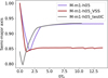 |
Fig. B.1 Migration tracks for the system M-m1-h05 in the standard configuration (purple line); with different boundary conditions (red line); with different initial conditions (gray line). |
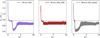 |
Fig. B.2 Density at resonances for the system M-m1-h05 in the standard configuration (purple line); with different boundary conditions (red line); with different initial conditions (gray line). |
All Tables
All Figures
|
Fig. 1 Semimajor axis (upper panels) and eccentricity (lower panels) as a function of the evolutionary time. The left panels show the light disk simulations, the right panels show the massive disk simulations. As indicated in the legend, the solid/dashed/dotted lines show the orbital parameters for simulations with 1 mJup/3 mJup/13 mJup planets. The different colors correspond to different disk aspect ratios. |
| In the text | |
|
Fig. 2 Simulation M-m1-h05. The color maps show the azimuthal average of the disk normalized density Σ/Σ0 (left panel) and of the disk eccentricity (right panel) as a function of the disk radius (x-axis) and of evolutionary time t/tν,0 (y-axis). The white line in both plots shows the planet migration track. |
| In the text | |
|
Fig. 3 Analysis of the migration behavior in simulation M-m1-h05. The left panel shows the semimajor axis as a function of the evolutionary time, with a zoom in the region where the planet changes its direction of migration, marked via the green dot. The other colored dots mark selected snapshots just before and after the change in migration direction. The middle-left panel shows the density profiles at the selected snapshots. The middle-right panel shows the disk (dark purple) and planet eccentricity (medium purple) evolution. The colored regions highlight the selected snapshots. The plot in the right panel illustrates the density ratio at the 1:2 and 1:3 resonances. |
| In the text | |
|
Fig. 4 Portion of the normalized torque responsible for the change in the semimajor axis as a function of the density ratio at the 1:2 and 1:3 resonances Σ1:2/Σ1:3. Different colors indicate different disk aspect ratios at 5 au, as indicated in the legend. Markers indicate the state of each simulation at t = 10 tν. The lines show the evolution of each simulation, whose start is shown by the circles. The inset shows the evolution track for the simulation M-m1-h05. The high (low) line opacity corresponds to the lower (higher) disk mass regimes. |
| In the text | |
|
Fig. 5 Migration track (left panel) and density profiles (right panel). The colored dots in the left panel show some selected snapshots for inward (orange), outward (light blue), and stalling (purple and pink) phase of migration. The density profiles in the right panel are shown in colors corresponding to the dots in the left panels. |
| In the text | |
|
Fig. 6 Portion of the normalized torque responsible for the change in the semimajor axis as a function of the gap-shape parameter, K. Different colors indicate different disk aspect ratios at 5 au, as indicated in the legend. Markers indicate the state of each simulation at t = 10 tν,0. The lines show the evolution of each simulation. The high (low) line opacity corresponds to the lower (higher) disk mass regimes. |
| In the text | |
|
Fig. 8 Portion of the normalized torque responsible for the change in the semimajor axis as a function of the gap-shape parameter, K. In the left panel, the plot shows the distribution of the simulations at t = 3 tν,0, while the right panel shows the distribution at t = 10 tν,0. The marker shape indicates the planet mass: 1 mJup (squares), 3 mJup (circles), and 13 mJup (diamonds). The colors indicate the disk aspect ratio at 5 au. Dashed markers indicate the massive disk simulations. The translucent markers indicate the systems entering a different migration regime with respect to that studied in this paper. |
| In the text | |
|
Fig. 9 Gap-shape parameter, K, map as a function of the local disk aspect ratio (y-axis) and planet mass (x-axis). Some reference values for K are highlighted via the gray contours (the “stalling region” is within the interval log(K) = [3.3, 4.1]). The brown-yellow area indicates the combination of h, α, mp that is expected to generate inward migration; the teal area shows the combination of parameters that is expected to correspond to outward migration. |
| In the text | |
|
Fig. 10 Evolution of Jupiter-mass planets in physical units for light (left) and massive (right) disks. Solid lines show simulation tracks, while dashed lines indicate predictions from the toy model of Scardoni et al. (2022) (W = 1, Klim = 3500). |
| In the text | |
|
Fig. 11 Normalized torque as a function of the gap-width parameter K′ = q2/αh3. |
| In the text | |
|
Fig. A.1 Ratio between the disk density at the 1:2 resonance and at the 1:3 resonance for all simulations with 1 mJup planets (colored lines), as indicated in each panel legend. The gray lines in each plot show the rate of change of the planet semimajor axis, |
| In the text | |
|
Fig. B.1 Migration tracks for the system M-m1-h05 in the standard configuration (purple line); with different boundary conditions (red line); with different initial conditions (gray line). |
| In the text | |
|
Fig. B.2 Density at resonances for the system M-m1-h05 in the standard configuration (purple line); with different boundary conditions (red line); with different initial conditions (gray line). |
| In the text | |
Current usage metrics show cumulative count of Article Views (full-text article views including HTML views, PDF and ePub downloads, according to the available data) and Abstracts Views on Vision4Press platform.
Data correspond to usage on the plateform after 2015. The current usage metrics is available 48-96 hours after online publication and is updated daily on week days.
Initial download of the metrics may take a while.