| Issue |
A&A
Volume 704, December 2025
|
|
|---|---|---|
| Article Number | A38 | |
| Number of page(s) | 17 | |
| Section | Interstellar and circumstellar matter | |
| DOI | https://doi.org/10.1051/0004-6361/202557095 | |
| Published online | 02 December 2025 | |
A multi-scale evolutionary study of molecular gas in STARFORGE
I. Synthetic observations of SEDIGISM-like molecular clouds
1
Max-Planck-Institut für Radioastronomie,
Auf dem Hügel 69,
53121
Bonn,
Germany
2
Argelander-Institut für Astronomie,
Auf dem Hügel 71,
53121
Bonn,
Germany
3
Department of Astronomy, The University of Texas at Austin,
Austin,
TX
78712,
USA
4
Centre for Modern Interdisciplinary Technologies, Nicolaus Copernicus University in Torun,
Wileńska 4,
87-100
Toruń,
Poland
5
National Centre for Nuclear Research,
Pasteura 7,
02-093
Warszawa,
Poland
6
Centre for Astrophysics and Planetary Science, University of Kent,
Canterbury
CT2 7NH,
UK
7
School of Physics & Astronomy, Cardiff University, Queen’s building, The parade,
Cardiff
CF24 3AA,
UK
★ Corresponding author: This email address is being protected from spambots. You need JavaScript enabled to view it.
Received:
4
September
2025
Accepted:
8
October
2025
Abstract
Molecular clouds (MCs) are active sites of star formation in galaxies, and their formation and evolution are largely affected by stellar feedback. This includes outflows and winds from newly formed stars, radiation from young clusters, and supernova explosions. High-resolution molecular line observations allow for the identification of individual star-forming regions and the study of their integrated properties. Moreover, state-of-the-art simulations are now capable of accurately replicating the evolution of MCs, including all key stellar feedback processes. We present 13CO(2–1) synthetic observations of the STARFORGE simulations produced using the radiative transfer code RADMC-3D, matching the observational setup of the SEDIGISM survey. From these synthetic observations, we identified the population of MCs using hierarchical clustering and analysed them to provide insights into the interpretation of observed MCs as they evolve. The flux distributions of the post-processed synthetic observations and the properties of the MCs, namely, radius, mass, velocity dispersion, virial parameter, and surface density, are consistent with those of SEDIGISM. Both samples of MCs occupy the same regions in the scaling relation plots; however, the average distributions of MCs at different evolutionary stages do not overlap on the plots. This highlights the reliability of our approach in modelling SEDIGISM and suggests that MCs at different evolutionary stages contribute to the scatter in observed scaling relations. We study the trends in MC properties, morphologies, and fragmentation over time to analyse their physical structure as they form, evolve, and are destroyed. MCs appear as small diffuse cloudlets in early stages, and this is followed by their evolution to filamentary structures before being shaped by stellar feedback into 3D bubbles and getting dispersed. These trends in the observable properties of MCs are consistent with other realisations of simulations and provide strong evidence that clouds exhibit distinct morphologies over the course of their evolution.
Key words: stars: winds, outflows / ISM: bubbles / ISM: clouds / ISM: supernova remnants
Member of the International Max Planck Research School (IMPRS) for Astronomy and Astrophysics at the Universities of Bonn and Cologne.
© The Authors 2025
 Open Access article, published by EDP Sciences, under the terms of the Creative Commons Attribution License (https://creativecommons.org/licenses/by/4.0), which permits unrestricted use, distribution, and reproduction in any medium, provided the original work is properly cited.
This article is published in open access under the Subscribe to Open model.
Open Access funding provided by Max Planck Society.
1 Introduction
The molecular gas in the interstellar medium (ISM) is hierarchically clustered in the form of molecular clouds (MCs; (Dobbs et al. 2014; Chevance et al. 2023)). Molecular clouds are turbulent magnetically supercritical (Crutcher 2012) structures with sizes of ~1–200 pc (Ballesteros-Paredes et al. 2020; Duarte-Cabral et al. 2021), mass M ~102−107 M⊙ (Rebolledo et al. 2012), surface densities Σ ~ 1–1000 M⊙ pc−2 (Barnes et al. 2018), and virial parameter (αvir) around unity (Fukui et al. 2008; Roman-Duval et al. 2010). They show various morphologies (Neralwar et al. 2022a), with filaments being the most ubiquitous (André et al. 2010; Li et al. 2016; Duarte-Cabral & Dobbs 2017; Arzoumanian et al. 2019; Colombo et al. 2021; Priestley & Whitworth 2022).
The evolution of MCs is often presented as being regulated by either SN-driven turbulence (Padoan et al. 2016; Lu et al. 2020) or hierarchical gravitational collapse (Ballesteros-Paredes et al. 2011; Vázquez-Semadeni et al. 2019). These mechanisms lead to the fragmentation and formation of dense cores, which further lead to the formation of protostars. Protostars accrete gas from the surrounding ISM, leading to feedback in the form of bipolar outflows (Bally 2016). These outflows (jets) are relatively collimated structures that heat and compress the gas as they inter-act with the surrounding ISM up to parsec scales (e.g. Duarte-Cabral et al. 2012; Skretas et al. 2023; Karska et al. 2025). Outflows can vary significantly in energetics, with momentum rates between 10−5 and 10−2 M⊙ kms−1 yr−1 for low-mass and O-type stars (e.g. Duarte-Cabral et al. 2013; Maud et al. 2015).
As the forming protostars move onto the main-sequence stage, they begin to drive isotropic stellar winds (Vink 2024), which help clear out the remaining gas in their envelope. Stellar winds form bubble-shaped cavities around stars (Weaver et al. 1977; Fierlinger et al. 2016; Ali et al. 2022) by releasing a significant amount of kinetic energy into the ISM (~1048 erg over the lifetime of the bubble, Luisi et al. 2021). In addition to stellar winds, high-energy radiation from massive stars (M ≥ 8 M⊙) ionises the surrounding gas, releasing thermal xsenergy (~1046 erg) and forming ionised (H II) regions (Simpson et al. 2012; Figueira et al. 2017; Santoro et al. 2022). Stellar winds and photoionising radiations are active during the main-sequence phase of stars (a few megayears) and play a major role in dispersing MCs (Rosen et al. 2020; Chevance et al. 2020). The last form of feedback, and perhaps one of the most important in setting the global conditions of the ISM in galaxies, are supernova explosions from massive stars (Geen et al. 2015; Lucas et al. 2020). Supernovae inject a large amount of energy (~1051 ergs) and drive the supersonic turbulence in the ISM on tens to hundreds of parsec scales. (Lu et al. 2020; Dubner & Giacani 2015).
Although various stellar feedback mechanisms have a significant impact on cloud formation, evolution, and dissolution (Chevance et al. 2023), observational studies of MCs rarely attempt to distinguish between clouds affected by different forms of feedback. Clouds are often generalised into a single population of quasi-static entities in near equilibrium (Colombo et al. 2019; Duarte-Cabral et al. 2021) and are collectively analysed using a scaling relation, such as those of Larson (1981) and Heyer et al. (2009). However, they are not necessarily hydrostatic structures, as the turbulence support (static clouds) and global hierarchical collapse (dynamical clouds) cloud formation models produce the same observational signatures (Vázquez-Semadeni et al. 2024). Studying the effects of local feedback events on cloud properties might provide some evidence in support of or in opposition to these models.
In the past decade, several high-resolution surveys of the Milky Way have revealed the intricate structure of MCs and allowed their properties to be resolved in detail (e.g. COHRS Dempsey et al. 2013, CHIMPS Rigby et al. 2016, SEDIGISM Schuller et al. 2021, and OGHReS Urquhart et al. 2024, 2025). Complementing such observations, state-of-the-art giant MC (GMC) simulations are now able to model the ISM at high resolution (e.g. SICLL Walch et al. 2015; Seifried et al. 2017, STARFORGE Grudić et al. 2021, and FIRE Hopkins et al. 2023) while including most of the physical phenomena related to star formation. Comparison of these observations and simulations requires mapping the simulations onto observational space using radiative transfer (e.g. RADMC-3D Dullemond et al. 2012) in order to model the emission that the simulated gas and stars would produce.
One goal of this paper is to use state-of-the-art simulations that incorporate all the relevant physics of star formation to produce synthetic observations that closely resemble observational data. We generated synthetic observations from the Star Formation in Gaseous Environments (STARFORGE) simulations following the observational setup of the SEDIGISM survey (Duarte-Cabral et al. 2021). Using RADMC-3D, we produced the 13CO(2–1) line-emission cubes from the simulations and used a dendrogram-based cloud identification technique to extract MCs. We thus evaluated the extent to which current simulations can reproduce the observed MCs. Through this work, we also aim to analyse the observable properties of MCs as they evolve and determine whether their distributions vary across different evolutionary stages in order to provide some insight into the interpretation of observational MC surveys. As the cloud properties are comparable with SEDIGISM, we were able to provide a direct comparison of the cloud properties as they evolve and are affected by stellar feedback.
The structure of the paper is as follows. In Section 2 we describe the STARFORGE simulations used for our analysis and the SEDIGISM survey, which we used as a observational comparative benchmark. In Section 3, we describe the methodology to create the synthetic observations from STARFORGE (Sect. 3.1) along with the post-processing of the data (Sect. 3.2). We then describe the dendrogram algorithm used to extract structures from these synthetic observation cubes in Sect. 3.3, and this is followed by the definition of MC properties. We present our results of a comparison of the clouds from the simulations and those from SEDIGISM in Sect. 4.1. We investigate the evolution of the properties and morphologies of clouds over time and connect them to the formation of stars in Sect. 4.2. We analyse the scaling relations to compare the correlation between STARFORGE and SEDIGISM cloud properties and understand the time evolution of clouds on these plots in Sect. 5. In Sect. 6, we explain the trends in the properties, morphology, and substructures of MCs over time and connect them to their observed counterparts. We conclude by summarising our work in Sect. 7.
2 Data
2.1 STARFORGE
The STARFORGE1 simulations are three-dimensional radiation magnetohydrodynamic (MHD) simulations that follow the evolution of GMCs, and they achieve spatial resolutions of a few tens of AU. These simulations model the formation, evolution, and dynamics of individual stars within a GMC, incorporating all forms of stellar feedback: jets, radiation, stellar winds, and supernovae. The simulation framework is built on the GIZMO code (Hopkins 2015), which uses a Lagrangian meshless finite mass method to solve MHD equations (Hopkins & Raives 2016). A comprehensive explanation of the numerical methods and validation tests is provided in Grudić et al. (2021).
We used the M2e4a2 suite of STARFORGE simulations (Table 1 of Guszejnov et al. 2022). It follows the evolution of a 20 000 M⊙ GMC2 to ~11 Myr and saves all the properties every 24.7 kyr, thus producing a total of 445 snapshots. Of the total number of snapshots, we analysed 410 that have significant 13CO(2–1) emission in order to identify dendrogram structures. The GMC was initiated as a uniform surface density sphere with R = 10 pc, αvir = 2, and T = 10 K surrounded by a diffuse medium (density contrast of 1000) in a (100 pc)3 box3. The gas was initiated as fully atomic, but the ionisation state rapidly converged to local equilibrium such that the interior of the cloud rapidly became fully molecular. The calculation we analysed includes the heating and cooling contributions from all key molecular, atomic, nebular, and continuum processes (see Hopkins et al. 2018, for more detail). Although the simulation does not explicitly follow the formation and destruction of H2, it computes the molecular gas fraction in each cell using a fitting function that depends on the gas metalicity and surface density (Krumholz & Gnedin 2011). We then derived the number density of molecular hydrogen by assuming that the molecular gas mass in each cell is composed of molecular hydrogen.
We restricted our analysis to the gas within the inner 60 pc of the simulation box, as that is sufficient to capture the 13CO(2–1) emission throughout the time evolution we studied. As the simulation progresses, the GMC collapses under self-gravity to form protostars (at 0.8 Myr) with outflows. Stars with photoionising radiation (at 2.7 Myr) and stellar winds (at 3.6 Myr) are then formed, and they disperse most of the GMC before the first supernova (at 9.8 Myr) occurs. This evolution follows a global hierarchical collapse scenario with various stellar feedback mechanisms that can contribute to the injection of local turbulence and provide support against local collapse (Grudić et al. 2022; Guszejnov et al. 2022).
2.2 SEDIGISM
The Structure, Excitation, and Dynamics of the Inner Galactic InterStellar Medium (SEDIGISM; see Schuller et al. 2017, 2021 for an overview) survey spans an area of 84 deg2 within the Galactic longitude range of −60° ≤ l ≤ + 18° and latitude |b| ≤ 0.5° (with some regional variations). It includes multiple molecular tracers specifically targeting the J = 2–1 transitions of 13CO and C18O. Observations were conducted from 2013 to 2017 using the 12 meter Atacama Pathfinder Experiment (APEX) telescope (Güsten et al. 2006). The survey provides a contiguous dataset divided into 77 data cubes, each covering approximately 2° × 1° and with a velocity coverage of −200 to 200 km s−1 and a pixel size of 9.5". The first data release (DR1) features 13CO observations with a full width at half maximum beam size of 28″ and a typical 1-σ sensitivity of 0.8–1.0 K per 0.25 km s−1.
Using this dataset, Duarte-Cabral et al. (2021) constructed a catalogue of 10663 MCs with their physical properties, further updated by Urquhart et al. (2021), Colombo et al. (2022), and Neralwar et al. (2022a). The MCs were identified using the Spectral Clustering for Interstellar Molecular Emission Segmentation (scimes) algorithm (v.0.3.2, Colombo et al. 2015, 2019). Duarte-Cabral et al. (2021) also defined a science sample that consists of well-resolved clouds with reliable distance estimates. We selected MCs from the science sample that are at distances between 2.5 and 3.5 kpc away for our comparative analysis. This distance range provides a sufficiently large sample size (of 835 clouds) with a consistent physical resolution (~0.3–0.5 pc) and minimises the effects of different sensitivities at different distances. In the following, we refer to these clouds as SEDIGISM clouds. We use the deconvolved equivalent radius (radius_dec_pc4), cloud mass (Mass), velocity dispersion (sigv_kms), virial parameter (alpha_vir), and surface density (Surf_density_dec_Mpc2) to compare SEDIGISM clouds to synthetic MCs identified in this paper (Sect. 4.1).
3 Methods
3.1 Radiative transfer
We used the RADMC-3D (version 2.0, Dullemond et al. 2012) radiative transfer code on STARFORGE simulation to obtain the position-position-velocity (PPV) 13CO(2–1) emission cubes that mimic the SEDIGISM survey. RADMC-3D uses the simulation data as input, including the distribution of the density, temperature, composition of the gas, and sources of radiation, and it generates a three-dimensional grid of points that are used to sample the environment and calculate the radiative transfer. We briefly outline the procedure in the following subsections.
3.1.1 Data preprocessing
We interpolated the STARFORGE data to a uniform grid with resolution 480 × 480 as input for RADMC-3D5, matching the resolution in SEDIGISM at a distance of ~3 kpc. The RADMC-3D inputs are gas temperature, velocity, and the number densities of 13CO and H2, which acts as a collision partner. The collisional rate coefficients for 13CO are provided by the Leiden Atomic and Molecular Database (LAMDA6). We obtained the number density of 13CO from the H2 number density estimated from the molecular gas fraction using an abundance ratio of H2/CO = 104 (typical of the inner Milky Way, Dame et al. 2001; Bolatto et al. 2013) and a constant isotopic ratio of 12CO/13CO = 42.6 (Jacob et al. 2020, at the Galactocentric radius of 5 kpc). We also applied a freeze-out criterion by setting the 13CO abundance ratio to 50% in regions with a gas temperature below 17 K and a gas density above 105cm−3 (Caselli et al. 1999; Lippok et al. 2013; Roueff et al. 2021). However, various temperature and density thresholds tested for the freeze-out criterion did not strongly affect the distribution of the 13CO(2–1) emission studied in this work. RADMC-3D calculates line profiles based on thermal broadening by default, but it allows for the inclusion of turbulent widths (microturbulence7). We calculated the microturbulence as the product of the velocity gradient in a cell and the size of the cell, where the velocity gradient for the cells is obtained using the numerical differentiation functionality of the MESHOID8 script.
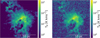 |
Fig. 1 Left: synthetic integrated 13CO(2–1) emission map created with RADMC-3D. Right: same map but after convolution and with the noise of sigma = 0.2 ± 0.02 K. |
3.1.2 RADMC-3D
The radiative transfer code RADMC-3D calculates line emission by obtaining the level population in each grid cell based on a line transfer model. We used the non-local thermodynamic equilibrium approximation together with the large velocity gradient mode and the escape probability method9. The 13CO(2–1) transition emits at 220.398 GHz, or 1360.227 μm. We used this as the central wavelength to obtain PPV cubes with 65 channels separated by 0.25 kms−1, leading to a velocity coverage of ±8 kms−1. We used the RADMC-3D image option with loadlambda to create PPV cubes of size 65 × 448 × 448 pixels at a distance of 3 kpc and a pixel size of 9.5″ (corresponding to 60 pc) in order to compare the SEDIGISM clouds directly (see Sect. 2.2) We also made use of second-order integrations while creating the image to avoid pixelation. For each snapshot, the 13CO(2–1) cubes were constructed for three different lines of sight along the x, y, and z directions (Appendix A) using the phi={90, 0, 0} and incl={90, 90, 0} parameters.
3.2 PPV cube post-processing
We post-processed the output PPV cube from RADMC-3D (Fig. 1, left) in order to replicate the characteristics of the SEDIGISM observations using the following procedure. First, the cube was convolved with a 2D Gaussian kernel with a full width at half maximum of 28″, corresponding to the APEX telescope beam at 220.398 GHz. The data from the noisy (first and last 50) channels of the SEDIGISM G305 cube were added to the cube as noise. To improve the signal-to-noise ratio, the data were spectrally smoothed at 0.5 kms−1 resolution and resampled to 0.25 kms−1 (Sect. 3.1.1 in Duarte-Cabral et al. 2021). An example of an original and post-processed cube is shown in Fig. 1.
To suppress the noise and prepare the data for the analysis of dendrograms, we applied the dilated masking method described in Grishunin et al. (2024), resulting in clean masked cubes (Appendix B). We performed two masking iterations as Grishunin et al. (2024) for robust data cleaning, with s2n_low = 2, s2n_high = 4, and s2n_vel = 3 for the first iteration and s2n_low = 2, s2n_high = 5, and s2n_vel = 3 for the second. The s2n_low follows the min_val parameter in Duarte-Cabral et al. (2021), setting the value of pixels whose emission is lower than 2σ of the local noise to zero. The higher value of s2n_high in the second iteration provides a stricter constraint to remove any spurious sources. These data processing steps allowed us to closely replicate the observed dataset of SEDIGISM (Sect. 4.1). Of the 445 snapshots, the first 35 (up to ~1 Myr) have no detectable 13CO(2–1) above the s2n_low limit. Our analysis is therefore limited to 410 snapshots, resulting in a total of 1230 synthetic data cubes for the three projections. Excluding the early snapshots minimises potential biases in the reproduction of the synthetic line emission that could arise from the initial settling of the cloud. By ~1 Myr, the gas density distribution reaches a quasi-equilibrium state, satisfying a log-normal distribution, which is expected for supersonically turbulent gas (Padoan et al. 1997; Lane et al. 2022).
3.3 Dendrograms and cloud properties
Dendrograms describe the distribution and nesting of isosurfaces in data cubes and have long been used to discretise molecular gas emission at different scales in observations (Colombo et al. 2019; Duarte-Cabral et al. 2021) and simulations (Offner et al. 2022). We used dendrograms (Rosolowsky et al. 2008) to segment the molecular gas in each snapshot into leaves, branches, and trunks. Leaves are structures formed by single local maxima in the gas distribution and are nested in branches, which in turn are nested in trunks. The trunks can be isolated structures without substructures or hierarchical structures with multiple substructures (Appendix D). Dilated masking sets the value of all noisy voxels to zero, setting the lower threshold of the dendrograms. We built the dendrograms using min_val = 0 and n_delta = 2 σrms, where σrms = 0.87 represents the mean rms noise in our data (Sect. 3.2). We set the min_pix using n_area = 3 and n_vchan =2 such that all structures are both spatially (i.e. at least three beams) and spectrally (span at least two velocity channels) resolved. We found a total of 3710 hierarchical trunks and refer to them as MCs throughout this work. The entirety of detectable 13CO(2–1) emission in a snapshot is referred to as the ‘molecular gas complex’ or the ‘entire 13CO(2–1) emission’. Additionally, the dendrograms store information about the nested structures (descendants) for every structure. We perform a quantitative analysis of these substructures (descendants) in each MC in Sect. 4.2.3.
The dendrogram analysis returned a catalogue of structures10 with their properties (Rosolowsky & Leroy 2006), which we used to derive other MC properties while assuming a heliocentric distance of 3 kpc. The most useful directly measured properties are the projected footprint area (A), the velocity dispersion (σr), and the total brightness temperature (TB). The effective radius is defined as ![Mathematical equation: $\[R_{eff}=\sqrt{A / \pi}\]$](/articles/aa/full_html/2025/12/aa57095-25/aa57095-25-eq1.png) and the deconvolved radius as
and the deconvolved radius as ![Mathematical equation: $\[R=\sqrt{R_{eff}^{2}-R_{beam}^{2}}\]$](/articles/aa/full_html/2025/12/aa57095-25/aa57095-25-eq2.png) , where Rbeam = 0.2 pc is the physical size of the beam11. The luminosity mass was estimated from the luminosity (L) as Mlum [M⊙] = αCO L [L⊙], where αCO = 22.43 M⊙ (K km s−1)−1 pc−2, estimated using X13CO(2–1) =
, where Rbeam = 0.2 pc is the physical size of the beam11. The luminosity mass was estimated from the luminosity (L) as Mlum [M⊙] = αCO L [L⊙], where αCO = 22.43 M⊙ (K km s−1)−1 pc−2, estimated using X13CO(2–1) = ![Mathematical equation: $\[1_{-0.5}^{+1}\]$](/articles/aa/full_html/2025/12/aa57095-25/aa57095-25-eq3.png) × 1021 cm−2 (K km s−1)−1 to be consistent with SEDIGISM. From this we derived the surface mass density Σ = Mlum/A and the virial parameter
× 1021 cm−2 (K km s−1)−1 to be consistent with SEDIGISM. From this we derived the surface mass density Σ = Mlum/A and the virial parameter ![Mathematical equation: $\[\alpha_{vir}=5 \sigma_{v}^{2} R / G M_{lum}\]$](/articles/aa/full_html/2025/12/aa57095-25/aa57095-25-eq4.png) , assuming a spherical and uniform cloud. The analysis presented in this paper uses deconvolved properties, although global trends are virtually unchanged by this choice.
, assuming a spherical and uniform cloud. The analysis presented in this paper uses deconvolved properties, although global trends are virtually unchanged by this choice.
We obtained the true molecular gas mass (M) directly from the simulation by projecting the H2 masses of gas cells onto the RADMC-3D code and summing over the pixels associated with a given dendrogram structure. The true molecular gas mass is not subject to observational biases or limitations (e.g. αCO factor) and includes the CO-dark and freeze-out regions. We used this mass to study the time evolution of clouds in Sect. 4.2.1, but their derived properties were calculated using Mlum to be consistent with the observations. STARFORGE also tracks the positions, mass, ages, and evolutionary stages of individual stars and protostars (Grudić et al. 2021). We recorded the number of newborn stars (protostars and stars younger than 250 kyr) and the mainsequence stars (with M > 2 M⊙) in each snapshot and used them to investigate the MC fragmentation in Sect. 4.2.3.
We analysed the cloud morphologies using the RJ plots (Clarke et al. 2022) algorithm, which is an extension of J plots (Jaffa et al. 2018). These algorithms classify pixelated structures into different morphologies based on the relationship between their mass distribution and moment of inertia. The J moments J1 and J2 are obtained by compairing the principal moments (I1 & I2) with those of a uniform surface density disc ![Mathematical equation: $\[\left(I_{0}=\frac{\mathrm{AM}}{4 \pi}\right)\]$](/articles/aa/full_html/2025/12/aa57095-25/aa57095-25-eq5.png) of the same area and mass:
of the same area and mass: ![Mathematical equation: $\[J_{i}=\frac{I_{0}-I_{i}}{I_{0}+I_{i}}\{i=1,2\}\]$](/articles/aa/full_html/2025/12/aa57095-25/aa57095-25-eq6.png) . The RJ moments R1 and R2 are obtained by rotating the J plot 45 degrees in the anticlockwise direction, and R2 was further normalised to remove the parameter space constraints given by |Ji| ≤ 1, resulting in
. The RJ moments R1 and R2 are obtained by rotating the J plot 45 degrees in the anticlockwise direction, and R2 was further normalised to remove the parameter space constraints given by |Ji| ≤ 1, resulting in ![Mathematical equation: $\[R_{1}=\frac{J_{1}-J_{2}}{2}\]$](/articles/aa/full_html/2025/12/aa57095-25/aa57095-25-eq7.png) and
and ![Mathematical equation: $\[R_{2}=\frac{J_{1}+J_{2}}{\sqrt{2}\left(\sqrt{2}-R_{1}\right)}\]$](/articles/aa/full_html/2025/12/aa57095-25/aa57095-25-eq8.png) . We note that R1 = 0 corresponds to a perfectly circular structure, with increasing values indicating progressively higher degrees of elongation. The term R2 measures the weight distribution of a structure compared to its centre of weight. The positive and negative values of R2 represent centrally overdense and underdense structures, respectively.
. We note that R1 = 0 corresponds to a perfectly circular structure, with increasing values indicating progressively higher degrees of elongation. The term R2 measures the weight distribution of a structure compared to its centre of weight. The positive and negative values of R2 represent centrally overdense and underdense structures, respectively.
4 Results
4.1 Validation of the synthetic dataset: Comparison with SEDIGISM
Before we could study the evolution of MCs using our sample of synthetic clouds, we first needed to ensure that our simulated sample was representative of the observed clouds in terms of properties and the probed parameter space. Therefore, we compared our synthetic MCs with those observed as part of the SEDIGISM survey (Duarte-Cabral et al. 2021). Figure 2 shows the flux distribution in each pixel for the SEDIGISM 13CO cubes and the emission of all STARFORGE snapshots along the three projections. The strong agreement between the two flux distributions serves as a validation that our synthetic emission maps replicate the SEDIGISM data to the first order.
Figure 3 shows the distribution of the integrated properties for our synthetic MCs and the SEDIGISM clouds. The good agreement between the two datasets for all properties indicates similar structural characteristics of the clouds in the two samples. This further highlights the relability of our approach in not only creating emission cubes similar to SEDIGISM but also identifying SEDIGISM-like clouds. However, this should not be confused as a single STARFORGE simulation replicating the entire diverse sample of clouds in SEDIGISM. Rather, due to robust data processing, our synthetic MCs occupy the same parameter space as SEDIGISM clouds.
The slight shift in the STARFORGE distributions towards higher values compared to SEDIGISM can be explained as follows. STARFORGE simulates an isolated GMC, and therefore the lowest level of dendrogram structures, i.e. hierarchical trunks, are called MCs. SEDIGISM, on the other hand, traces the larger gas structures in the Galaxy, and every dendrogram structure (e.g. non-overlapping trunks, branches, or leaves) is considered a cloud if it complies with the clustering criteria set by the segmentation algorithm. Using the same cloud identification criteria as SEDIGISM, i.e. the SCIMES algorithm (Colombo et al. 2019) is not suitable for this study. This is mainly due to the relatively small spatial coverage of each snapshot, which causes SCIMES to identify branches within the trunks as MCs, making the extracted clouds significantly smaller than those of SEDIGISM. The exclusion of leaves constrains the lower limit to the properties of our synthetic MCs. Despite these differences, our MCs are consistent with those in SEDIGISM (Figs. 8 and 9).
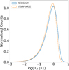 |
Fig. 2 Comparison between the flux values for the noisy pixels from all the STARFORGE snapshots along all three projections and the complete SEDIGISM survey (13CO(2–1) emission). |
4.2 Time evolution of MCs
The aim of this section is to understand the changes in the structure and properties of MCs as they evolve and are affected by different stellar feedback mechanisms (Fig. 4). To highlight the broader evolutionary trend, we binned the MCs based on the evolutionary time. Each bin corresponds to ~250 kyr and contains a total of 30 data cubes (three projections per snapshot). The evolution of properties of individual MCs is illustrated in the Appendix A. The following subsections focus on the general trends in integrated properties of the clouds (Sect. 4.2.1), their morphologies (Sect. 4.2.2), and substructures (Sect. 4.2.3). The corresponding figures (Figs. 5, 6 and 7) also show the onset of different stellar feedback mechanisms indicated on the time axis.
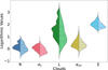 |
Fig. 3 Comparison of MC properties from STARFORGE (left side violins) and SEDIGISM (right side violins). The properties are radius (R), velocity dispersion (σv), luminosity (L), virial parameter (αvir), and surface density (Σ). The horizontal dashed lines represent the quartiles of the distributions. |
4.2.1 Integrated properties
In this section, we analyse the integrated properties of MCs as a function of time, over the ~11 Myr covered by the simulations. Figure 5 shows that the radius, mass, luminosity, and surface density properties follow each other closely, which is expected because larger MCs are more massive on average (Larson 1981; Kauffmann et al. 2010). The similar trends of molecular gas mass and 13CO luminosity distributions over time confirm that our results are not significantly affected by the choice of canonical 13CO abundances (see Sect. 3.1.1). The four properties show a steady increase until ~5, as progressively more 13CO(2–1) is above the detection limit. The increase represents the active growth of the MCs as they transition from newly formed small diffuse cloudlets to large, massive, and dense MCs (illustrated in Fig. 4). The increase in mass is also influenced by the transition of the gas from the atomic to the molecular phase and is a key characteristic of the global hierarchical collapse model (Shimajiri et al. 2019; Vázquez-Semadeni et al. 2019). The 6 Myr transition marks the beginning of gas expulsion and cloud dispersal by stellar feedback, as noted by the decrease in the average properties. This is supported by the significant increase in the number of clouds at ~7 Myr, which suggests that the gas is being removed and eroded from within and around clouds, resulting in a higher number of small cloud fragments (Sect. 7). These trends in MC properties are also seen in other simulation sets; however, their onset and duration vary depending on the initial conditions (Appendix E).
The velocity dispersion distribution remains relatively flat until ~6 Myr and then decreases. The initial high values for some MCs are largely a result of the initial supersonic turbulence, with a possible contribution from the momentum injected by the protostellar outflows. The average virial parameter decreases from ~10 to ~2 during the first 5 Myr and remains relatively constant throughout most of the evolution (Fig. 5). These distributions are not significantly affected by the growth and dispersal of MCs. However, they show peaks at ~2 Myr and ~10 Myr, which are also seen in the surface density distribution. The peaks correspond to the formation of turbulent gas structures and the onset of the first supernova, respectively. Supernovae inject turbulence into the ISM and produce relatively dense MCs in an environment that has mostly been dispersed by stellar winds and radiation. However, they do not significantly alter the general trends in the MC properties (Grudić et al. 2022).
 |
Fig. 4 Moment 0 maps of 13CO(2–1) at different evolutionary times. The background grey scale represents the H2 gas density with 13CO(2–1) emission overlaid as viridis maps (molecular gas complex), and the coloured contours represent different MCs (dendrogram trunks), with red contours representing the largest MCs (R) in the cube. The 13CO(2–1) maps for multiple snapshots along different projections are presented in Appendix B. |
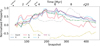 |
Fig. 5 Normalised medians of MC properties (log scales) as a function of time. The properties shown are radius (R), velocity dispersion (σv), molecular gas mass (M), virial parameter (αvir), surface mass density (Σ), and luminosity (L). The count refers to the total number of clouds in a time bin. The normalisation process included subtracting the initial value (first bin) of the property from it, and this was followed by a min-max standardisation. The symbols on the top represent the times at which outflows, photoionisation radiation, stellar winds, and supernovae begin in the simulation. |
4.2.2 Morphology
In this section, we study how the morphology of the MCs varies over time under the effect of various stellar feedback mechanisms. We used the RJ plots algorithm (Sect. 3.3) to analyse the morphology of the entire 13CO(2–1) emission in the simulation box as well as the individual MCs as they evolve over time (Fig. 6). The MCs show a large scatter in R1 and R2 at all times, as cloud structures present a continuous spectrum rather than discrete classes. We therefore binned the MCs following the same criteria as used in Sect. 4.2.1 in order to analyse the overall morphological changes and present the scatter plots in Appendix A. We also analysed the R1 and R2 moments for molecular gas complexes showing the structure of the entire emission in a snapshot.
Figure 6 shows that, on average, the clouds (both the individual MCs and the molecular gas complexes) have different elongations (R1) along the different projections. This is expected, as they evolve in a unisotropic environment, which causes them to evolve asymmetrically. However, this difference is not very significant for individual MCs, as shown by the large scatter in Fig. A.1 (bottom left). The trends in R2 are similar along the three projections, which highlights that the internal structure of the clouds appears the same regardless of the viewing angle.
The large average values of R1 for the MCs throughout most of the simulation highlight the ubiquitousness of filamentary structures (solid lines in Fig. 6, top). A notable trend in the distribution of R1 is a peak occurring in the 3–6 Myr range, suggesting an elongated shape for CO emission in snapshots (Fig. 4, centre). The increase in elongation is more dominant in one projection direction, suggesting that the molecular gas complex is collapsing faster along one axis. Although the average value of R1 for MCs increases after 6 Myr, this is not the case for molecular gas complexes. It points towards the emergence of filamentary MCs within feedback-affected spherical bubble-like regions and potentially indicates the formation of intra-cloud filaments. However, this increase should be interpreted with caution due to the large scatter in R1 among individual MCs. The distribution of R2 for the molecular gas complexes shows a constant increase until ~6 Myr, which is then followed by a constant decrease. The rise in central concentration (R2) is in agreement with the gravitational collapse of the simulated GMC. The decrease signifies the dispersion of the molecular gas due to stellar feedback, leading to centrally underdense bubble-like structures (Fig. 4, right). The increase in R2 along all three projections suggests that these MCs represent 3D bubbles rather than 2D rings (illustrated in Appendix B).
The different morphologies of the clouds for different projections reveal the anisotropy of the MCs. The anisotropy is driven by a combination of the initial turbulence, magnetic fields, and various stellar feedback events. A caveat of STARFORGE is that it assumes an isolated cloud and does not account for galacticscale processes, such as gas accretion and the galactic potential. However, we expect the galactic potential to have a minor effect on the cloud scale over a timescale of 10 Myr. Although we see the trends in the morphology for the entire 13CO emission in snapshots, the individual MCs on average remain elongated centrally concentrated structures throughout the simulation. Visual analysis further confirmed their filamentary and clumpy nature (Appendix B) during most of their lifetime (~3–7) Myr.
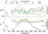 |
Fig. 6 Morphological analysis of the MCs (solid line) and molecular gas complexes (points) in different snapshots. R1 represents the degree of elongation, and R2 represents the degree of central concentration. The lines represent the R1 and R2 values for the MCs, and the scatter points represent the same for the molecular gas complexes, i.e. entire 13CO(2–1) emission in a snapshot, obtained using the projections along the three axes. The colour scheme is the same as in Fig. 3. |
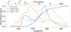 |
Fig. 7 Quantitative representation of MCs (counts), their substructures (dendrogram descendants), the newborn stars (age < 250 kyr), and the main-sequence stars more massive than 2M⊙ as a function of time. The values are normalised using a min–max standardisation. |
4.2.3 MC substructures
The fragmentation of MCs is often attributed to various stellar feedback mechanisms (Mazumdar et al. 2021; Grishunin et al. 2024); however, fundamental questions about the physics responsible for fragmenting MCs are still open. Analysing the number of MCs, their substructures, and stars provides information about how the MCs fragment to form dense substructures that lead to star formation, which in turn produces stellar feedback and disperses these gas structures. Here, we present a quantitative analysis of the substructures within our MCs. The substructures are stored by the dendrogram algorithm as descendants and represent subparsec-scale compact structures, which are typically referred to as clumps. Figure 7 shows an increase in the number of MCs and their substructures around (~3 Myr), representing progressively more emission that is above the noise level. The second peaks (~7–8 Myr) in both distributions are the result of gas dispersion by stellar feedback.
We also analysed the number of stars and protostars with ages less than 250 kyr and collectively refer to these as newborn stars. These reflect the instantaneous star formation rate of the clouds, with the 3–7 Myr period representing the peak of star formation activity. The newborn stars evolve to the main sequence, producing stellar winds and photoionising radiation. The stellar evolution is a strong function of their mass (Hosokawa et al. 2011), and a large number of low-mass stars remain in the main-sequence phase throughout the lifetime of the simulated GMC, seen as a constant increase in the number of stars over time (Fig. 7).
The significant increase in the number of stars at ~5 Myr is followed by peaks in the number of substructures (7 Myr) and MCs (8 Myr). Stellar winds and radiation from individual stars disperse and expel gas in their neighbourhood, fragmenting dense gas structures (6–7 Myr; Fig. 4). Over time, the feedback becomes stronger and erodes these fragmented clumps, causing them to decrease in number (>7 Myr). This strong gas dispersal affects the entire MC and leads to the removal of gas between dense MCs, i.e. the entire 13CO emission is identified as multiple small MCs instead of a single continuous structure, or trunk (7–8 Myr). These smaller MCs are dispersed over time as a result of continuous feedback events (>8 Myr). The lack of a dense molecular gas further decreases the number of embedded stars.
5 Scaling relations
The scaling relations (Larson’s and Heyer’s) show the correlations between the physical properties of clouds. Larson’s first relation, originally derived from the analysis of numerous MCs by Larson (1981), was later refined by Solomon et al. (1987), resulting in the relation σv = 0.74 L0.5 (discussed in Colombo et al. 2019). The spatial and velocity structures of MCs following power laws are often considered a proof of universal cloud turbulence (Padoan et al. 2016). It is a simplification of Kolmogorov’s law for turbulence, indicating that larger clouds exhibit broader linewidths. Larson’s laws individually do not provide information about the virial state of a cloud. To take this into account, Heyer et al. (2009) combined Larson’s second and third laws, creating Heyer’s relation, which compares the surface density of a cloud with its scaling parameter ![Mathematical equation: $\[\left(\sigma_{v}^{2} / R \propto \Sigma\right)\]$](/articles/aa/full_html/2025/12/aa57095-25/aa57095-25-eq9.png) .
.
We present the two scaling relations for our MCs and compare them with the SEDIGISM clouds in Figs. 8 and 9. The synthetic MC distribution shows an almost complete overlap with the 3-σ kernel density estimator for SEDIGISM clouds. This provides strong evidence that the MCs from our synthetic observations have global properties similar to those of real clouds. Moreover, this shows that the correlation of properties is consistent across both samples. That is, similar-sized MCs have similar velocity dispersions, leading to their overlap on the scaling relation plots.
Figure 8 shows an increase in the average size and linewidth of the clouds up to ~6 Myr. This is largely a result of the formation of dense gas structures that merge and result in progressively more 13CO(2–1) emission being detectable. In addition, stellar feedback mechanisms drive the velocities in the MCs and expand them, resulting in larger sizes and linewidths over time. At evolutionary times beyond ~6 Myr, stellar feedback mechanisms begin to disperse the gas significantly, resulting in the identification of smaller MCs. This appears as a sharp drop in the average velocity dispersion followed by a gradual decrease in their size. The higher values in the average velocity dispersion at early times (<6 Myr) for similar-sized structures are most likely due to the initial supersonic turbulence injected in the simulation.
Figure 9 highlights an initial trend of MCs as they transform from underdense and highly supervirial structures to denser virialised structures. The decrease in the average scaling ratio (σ2/R) is due to the significant increase in the MC radius compared to the velocity dispersion. The erosion of MCs due to feedback after 6 Myr causes a horizontal shift in Fig. 9 towards lower surface densities and higher virial parameters.
Molecular clouds are often analysed collectively in scaling relation plots, which typically show a large scatter (Colombo et al. 2019; Duarte-Cabral et al. 2021). Neralwar et al. (2022b) have shown that the cloud morphology and internal substructures influence their distribution in these relations and hypothesised that the different morphologies might correspond to different evolutionary stages. Figures 8 and 9 show that MC populations at different evolutionary times occupy different positions in the scaling relation plots. This suggests that the large scatter in the scaling relations could be due to the ensemble of observed MCs being at different stages of their evolution. SEDIGISM clouds could have gone through a diversity of physical conditions, as they are influenced by the larger Galactic environment and feedback events and follow various evolutionary paths. The gas flows and the effects of external factors are not simulated in STARFORGE. However, our MCs lie in the same parameter space as SEDIGISM, and the simulation traces all relevant physics of star formation at parsec scales. Therefore, at least some of the SEDIGISM clouds follow an evolutionary path similar to that of our MCs. When combined with the fact that MC morpholgies evolve over time (Sect. 4.2.2), our results support the hypothesis proposed by Neralwar et al. (2022b).
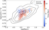 |
Fig. 8 Size-linewidth relation (σv versus R) for our MCs (scatter points), colour-coded with respect to the time elapsed (in Myr) since the start of the simulation. The squares represent medians of distributions in ~1 Myr bins. The black contours represent the 1σ, 2σ, 3σ levels for the SEDIGISM clouds. The dashed line represents Larson’s first relation (Larson 1981; Solomon et al. 1987). |
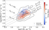 |
Fig. 9 Scaling relation between |
![Mathematical equation: $\[\sigma_v^2 / R\]$](/articles/aa/full_html/2025/12/aa57095-25/aa57095-25-eq10.png)
6 Discussion
6.1 The life cycle of synthetic MCs and their observed counterparts
The distribution of integrated properties, morphology, and fragmentation show that the MCs evolve from small, diffuse structures to dense filamentary structures before being dispersed by stellar feedback. They appear as filamentary and clumpy structures throughout most of their lifetimes, which is consistent with other simulations (e.g. Clarke et al. 2017). The smaller structures they host collapse and form stars even though the parent MC appears unbound (αvir ≫ 1). The stars produce stellar feedback that disperses the molecular gas, resulting in smaller, less massive diffuse structures. The presence of MCs as small clumps, filamentary structures, and bubble-like structures is also supported by observations (Neralwar et al. 2022a).
The initial turbulence in the simulations produces overdensities that become denser over time because of gravitational collapse. These MCs (<3 Myr) appear as small, diffuse, low mass, gravitationally unbound (αvir ~ 10) and approximately spherical structures. We refer to them as MCs following their definition as hierarchical trunks to be consistent throughout the paper; however, they are closer to starless molecular gas clumps in observations (e.g. starless clumps in Traficante et al. 2018 and quiescent clumps in Urquhart et al. 2022).
Molecular clouds at 3–7 Myr appear as large filamentary structures with dense clumps. The entire 13CO(2–1) emission in the simulation box appears as a single (or a few) large MC(s) since most of the gas in the simulation domain is molecular12. These represent a majority of the MCs detected in observational surveys (Molinari et al. 2010; Arzoumanian et al. 2011; Colombo et al. 2021; Neralwar et al. 2022a; Ge et al. 2023). The long lives of filamentary MCs are often attributed to continuous gas flows from the larger environment onto small-scale clumps through the filaments (Gómez & Vázquez-Semadeni 2014). Peretto et al. (2023) have shown that the substructures within the MCs produce a deep gravitational potential and accrete the gas from the filament and thus dynamically decouple from the MCs in order to grow faster. The formation of these dense clumps13 leads to a central infall of gas along the filament, which feeds the clumps, forms new small clumps, and causes turbulent movements (previously discussed in Gong et al. 2018; Lu et al. 2018; Williams et al. 2018; Krumholz & McKee 2020). The higher number of dense clumps results in an accelerated formation of protostars and stars (Fig. 7; 4–6 Myr).
Stellar winds and radiation become more effective throughout the simulation domain after ~6 Myr, resulting in gas expulsion and dispersion. These phenomena result in the 13CO(2–1) emission appearing as centrally underdense structures with a shell-like morphology. These 3D bubble-like clouds are widely studied as wind- and radiation-driven bubbles (Churchwell et al. 2004; Palmeirim et al. 2017; Tiwari et al. 2021) associated with H II regions (Neupane et al. 2024) and classified as the last evolutionary stage of clouds (Kawamura et al. 2009). Feedback disperses most of the 13CO emission by ~8 Myr, causing the broken shells to be identified as individual MCs. The formation of massive stars at ~3 Myr and most of the 13CO(2–1) emission being dispersed by ~8 Myr agrees with the fast dispersal of MCs by feedback (up to ~5 Myr, Kruijssen et al. 2019; Chevance et al. 2020; Figueira et al. 2020; Knutas et al. 2025).
6.2 Caveats and outlooks
STARFORGE simulates an isolated GMC within a closed box with a fixed total gas mass (2 × 10⁴M⊙) that restricts the upper mass limit of the MCs. Moreover, the simulation does not track the real-time abundance of CO, so the use of canonical abundance values and ad hoc freeze-out prescriptions is a simplification. This results in under- or overestimation of the real abundances, thus introducing an uncertainty on the measured Mlum from the synthetic observations and potentially skewing these distributions. To minimise this error, we set the CO abundance to zero in regimes where it can freeze out. We also set strict constraints while performing dilated masking (Sect. 3.2) and chose only the hierarchical trunks (Sect. 3.3) as MCs to avoid spurious sources. Inclusion of a chemical network in the simulations or radiative transfer could improve the accuracy of property estimates, but this goes beyond our current scope and does not significantly affect our overall analysis (Appendix C).
Predicting the evolutionary stages of SEDIGISM MCs based on their properties and morphology might be possible since our MCs share the same parameter space as SEDIGISM (Sect. 5). However, the degeneracy in these distributions on either side of the 6 Myr peak, visible as the large scatter in the scaling relation plots, makes this task extremely challenging when using only 13CO(2–1) observations. The early MCs show an H2 envelope (Fig. B.2) that could be traced with diffuse gas tracers such as 12CO, thus separating them from the feedback-affected MCs (Fig. B.3). Moreover, an analysis of the dense gas structures within MCs using tracers such as N2H+ and NH3 could reveal the fragmentation trends and aid in the evolutionary classification of the MCs. However, such a multi-wavelength study is beyond the scope of this work.
Observational works often perform multi-wavelength studies using tracers of dense gas, young stellar objects, and HII regions in order to classify MCs and clumps into various evolutionary stages (Kawamura et al. 2009; Traficante et al. 2018; Urquhart et al. 2022; Watkins et al. 2025). In a follow-up paper, we will study how clumps (dendrogram branches) and cores (dendrogram leaves) within our MCs are affected by various stellar feedback mechanisms (similar to Neralwar et al. 2024). This will improve our understanding of the evolution of the molecular gas structures from clouds to core scales. We will also compare these gas structures with their observed counterparts in observations at various evolutionary stages (Urquhart et al. 2022) to understand the degree to which such multi-wavelength analysis are able to predict the evolutionary stages of gas structures.
7 Summary and conclusions
In this paper, we have created synthetic observations from a 20 000 M⊙ STARFORGE simulation modelled after the SEDIGISM survey. We used the RADMC-3D radiative transfer code to convert the gas density cubes into 13CO(2–1) emission maps and performed a dendrogram analysis to identify MCs. We analysed this sample of synthetic MCs and investigated the trends in properties, morphology, and substructures to understand how MCs evolve under the effects of different stellar feedback mechanisms.
The flux distributions of the SEDIGISM ppv cubes and our synthetic data cubes are in strong agreement, validating the replication of the SEDIGISM data to the first order. The properties of the synthetic MCs show good agreement with the SEDIGISM clouds, and the two samples fill the same parameter space in the scaling relation plots, which further confirms the robustness of our approach. Although the two cloud samples show an overall good agreement, the sythetic MCs reproduce only a subset of the diversity seen in the observations. Moreover, synthetic MCs at different evolutionary stages occupy distinct regions of the scaling relation plots, suggesting that evolutionary time plays a significant role in driving the observed scatter.
We studied the formation, evolution, and destruction of MCs through variations in their observable properties. The initial turbulence in the simulations creates gas overdensities that collapse under self-gravity and are detected as 13CO(2–1) emission. These reflect the early cloudlets in observations that accrete gas from the larger environment and appear as moderately dense gas structures. Gas flows from large to small scales shape MCs into elongated filamentary structures with multiple substructures. The fractal substructures in MCs form stars, which eject matter and radiation into the surrounding environment, driving the formation of gas bubbles. These 3D bubble-like MCs are often associated with stellar winds, radiation, and H ir regions. Our analysis presents MCs as evolving from small, diffuse structures to dense filamentary MCs followed by 3D gas bubbles, and these evolutionary trends are consistent with simulations initialised differently. This confirms the key hypothesis from our previous observational work that MCs evolve from concentrated to elongated to ring-like structures.
In conclusion, we have produced 13CO(2–1) synthetic observations modelling the SEDIGISM survey using the STARFORGE simulations that include all the relevant physics for star formation. By analysing the properties, morphologies, and fragmentation trends of MCs, we have shown that they evolve from small, diffuse structures to dense filamentary structures to bubble-like structures. The distributions of MCs occupy different parameter spaces in the scaling relation plots, suggesting that they drive the scatter in the observed scaling relations. In an upcoming paper, we will study the effect of individual feedback mechanisms – outflows, stellar winds, radiation, supernovae – on these MCs and their substructures. We will also explore the possibility of compairing the structures at different evolutionary stages in simulations and observations.
Data availability
Movies associated to Appendix B are available at http://www.aanda.org
Movies
Movie 1 associated with Appendix B Access Supplementary Material
Movie 2 associated with Appendix B Access Supplementary Material
Movie 3 associated with Appendix B Access Supplementary Material
Acknowledgements
The authors thank the anonymous referee for a constructive report, which has significantly improved the quality of the manuscript. KN thanks Prof. Stefanie Walch-Gassner, Dr. Daniel Seifried, and Dr. Piyush Sharda for helpful discussions. AK acknowledges support from the Polish National Science Center SONATA BIS grant No. 2024/54/E/ST9/00314. MF acknowledges support from the Polish National Agency for Academic Exchange grant No. BPN/BEK/2023/1/00036/DEC/01 and from the Polish National Science Centre SONATA grant No. 2022/47/D/ST9/00419. S.N. gratefully acknowledges the Collaborative Research Center 1601 (SFB 1601 sub-project B1) funded by the Deutsche Forschungsgemeinschaft (DFG, German Research Foundation) – 500700252.
References
- Ali, A. A., Bending, T. J. R., & Dobbs, C. L. 2022, MNRAS, 510, 5592 [NASA ADS] [CrossRef] [Google Scholar]
- André, P., Men’shchikov, A., Bontemps, S., et al. 2010, A&A, 518, L102 [NASA ADS] [CrossRef] [EDP Sciences] [Google Scholar]
- Arzoumanian, D., André, P., Didelon, P., et al. 2011, A&A, 529, L6 [NASA ADS] [CrossRef] [EDP Sciences] [Google Scholar]
- Arzoumanian, D., André, P., Könyves, V., et al. 2019, A&A, 621, A42 [NASA ADS] [CrossRef] [EDP Sciences] [Google Scholar]
- Ballesteros-Paredes, J., Hartmann, L. W., Vázquez-Semadeni, E., Heitsch, F., & Zamora-Avilés, M. A. 2011, MNRAS, 411, 65 [NASA ADS] [CrossRef] [Google Scholar]
- Ballesteros-Paredes, J., André, P., Hennebelle, P., et al. 2020, Space Sci. Rev., 216, 76 [Google Scholar]
- Bally, J. 2016, ARA&A, 54, 491 [Google Scholar]
- Barnes, P. J., Hernandez, A. K., Muller, E., & Pitts, R. L. 2018, ApJ, 866, 19 [NASA ADS] [CrossRef] [Google Scholar]
- Bolatto, A. D., Wolfire, M., & Leroy, A. K. 2013, ARA&A, 51, 207 [CrossRef] [Google Scholar]
- Caselli, P., Walmsley, C. M., Tafalla, M., Dore, L., & Myers, P. C. 1999, ApJ, 523, L165 [Google Scholar]
- Chevance, M., Kruijssen, J. M. D., Hygate, A. P. S., et al. 2020, MNRAS, 493, 2872 [NASA ADS] [CrossRef] [Google Scholar]
- Chevance, M., Krumholz, M. R., McLeod, A. F., et al. 2023, in Astronomical Society of the Pacific Conference Series, 534, Protostars and Planets VII, eds. S. Inutsuka, Y. Aikawa, T. Muto, K. Tomida, & M. Tamura, 1 [Google Scholar]
- Churchwell, E., Whitney, B. A., Babler, B. L., et al. 2004, ApJS, 154, 322 [NASA ADS] [CrossRef] [Google Scholar]
- Clarke, S. D., Whitworth, A. P., Duarte-Cabral, A., & Hubber, D. A. 2017, MNRAS, 468, 2489 [Google Scholar]
- Clarke, S. D., Jaffa, S. E., & Whitworth, A. P. 2022, MNRAS, 516, 2782 [NASA ADS] [CrossRef] [Google Scholar]
- Colombo, D., Rosolowsky, E., Ginsburg, A., Duarte-Cabral, A., & Hughes, A. 2015, MNRAS, 454, 2067 [NASA ADS] [CrossRef] [Google Scholar]
- Colombo, D., Rosolowsky, E., Duarte-Cabral, A., et al. 2019, MNRAS, 483, 4291 [NASA ADS] [CrossRef] [Google Scholar]
- Colombo, D., König, C., Urquhart, J. S., et al. 2021, A&A, 655, L2 [NASA ADS] [CrossRef] [EDP Sciences] [Google Scholar]
- Colombo, D., Duarte-Cabral, A., Pettitt, A. R., et al. 2022, A&A, 658, A54 [NASA ADS] [CrossRef] [EDP Sciences] [Google Scholar]
- Crutcher, R. M. 2012, ARA&A, 50, 29 [Google Scholar]
- Dame, T. M., Hartmann, D., & Thaddeus, P. 2001, ApJ, 547, 792 [Google Scholar]
- Dempsey, J. T., Thomas, H. S., & Currie, M. J. 2013, ApJS, 209, 8 [NASA ADS] [CrossRef] [Google Scholar]
- Dobbs, C. L., Krumholz, M. R., Ballesteros-Paredes, J., et al. 2014, in Protostars and Planets VI, eds. H. Beuther, R. S. Klessen, C. P. Dullemond, & T. Henning, 3 [Google Scholar]
- Duarte-Cabral, A., & Dobbs, C. L. 2017, MNRAS, 470, 4261 [NASA ADS] [CrossRef] [Google Scholar]
- Duarte-Cabral, A., Chrysostomou, A., Peretto, N., et al. 2012, A&A, 543, A140 [NASA ADS] [CrossRef] [EDP Sciences] [Google Scholar]
- Duarte-Cabral, A., Bontemps, S., Motte, F., et al. 2013, A&A, 558, A125 [NASA ADS] [CrossRef] [EDP Sciences] [Google Scholar]
- Duarte-Cabral, A., Colombo, D., Urquhart, J. S., et al. 2021, MNRAS, 500, 3027 [Google Scholar]
- Dubner, G., & Giacani, E. 2015, A&A Rev., 23, 3 [NASA ADS] [CrossRef] [Google Scholar]
- Dullemond, C. P., Juhasz, A., Pohl, A., et al. 2012, RADMC-3D: a multi-purpose radiative transfer tool, Astrophysics Source Code Library [record ascl:1202.015] [Google Scholar]
- Fierlinger, K. M., Burkert, A., Ntormousi, E., et al. 2016, MNRAS, 456, 710 [NASA ADS] [CrossRef] [Google Scholar]
- Figueira, M., Zavagno, A., Deharveng, L., et al. 2017, A&A, 600, A93 [NASA ADS] [CrossRef] [EDP Sciences] [Google Scholar]
- Figueira, M., Zavagno, A., Bronfman, L., et al. 2020, A&A, 639, A93 [NASA ADS] [CrossRef] [EDP Sciences] [Google Scholar]
- Fukui, Y., Kawamura, A., Minamidani, T., et al. 2008, ApJS, 178, 56 [Google Scholar]
- Ge, Y., Wang, K., Duarte-Cabral, A., et al. 2023, A&A, 675, A119 [NASA ADS] [CrossRef] [EDP Sciences] [Google Scholar]
- Geen, S., Rosdahl, J., Blaizot, J., Devriendt, J., & Slyz, A. 2015, MNRAS, 448, 3248 [Google Scholar]
- Gómez, G. C., & Vázquez-Semadeni, E. 2014, ApJ, 791, 124 [Google Scholar]
- Gong, Y., Li, G. X., Mao, R. Q., et al. 2018, A&A, 620, A62 [NASA ADS] [CrossRef] [EDP Sciences] [Google Scholar]
- Grishunin, K., Weiss, A., Colombo, D., et al. 2024, A&A, 682, A137 [NASA ADS] [CrossRef] [EDP Sciences] [Google Scholar]
- Grudić, M. Y., Guszejnov, D., Hopkins, P. F., Offner, S. S. R., & Faucher-Giguère, C.-A. 2021, MNRAS, 506, 2199 [NASA ADS] [CrossRef] [Google Scholar]
- Grudić, M. Y., Guszejnov, D., Offner, S. S. R., et al. 2022, MNRAS, 512, 216 [CrossRef] [Google Scholar]
- Güsten, R., Nyman, L. Å., Schilke, P., et al. 2006, A&A, 454, L13 [NASA ADS] [CrossRef] [EDP Sciences] [Google Scholar]
- Guszejnov, D., Grudić, M. Y., Hopkins, P. F., Offner, S. S. R., & Faucher-Giguère, C.-A. 2021, MNRAS, 502, 3646 [NASA ADS] [CrossRef] [Google Scholar]
- Guszejnov, D., Grudić, M. Y., Offner, S. S. R., et al. 2022, MNRAS, 515, 4929 [Google Scholar]
- Heyer, M., Krawczyk, C., Duval, J., & Jackson, J. M. 2009, ApJ, 699, 1092 [Google Scholar]
- Holdship, J., Viti, S., Jiménez-Serra, I., Makrymallis, A., & Priestley, F. 2017, AJ, 154, 38 [NASA ADS] [CrossRef] [Google Scholar]
- Hopkins, P. F. 2015, MNRAS, 450, 53 [Google Scholar]
- Hopkins, P. F., & Raives, M. J. 2016, MNRAS, 455, 51 [NASA ADS] [CrossRef] [Google Scholar]
- Hopkins, P. F., Wetzel, A., Kereš, D., et al. 2018, MNRAS, 480, 800 [NASA ADS] [CrossRef] [Google Scholar]
- Hopkins, P. F., Wetzel, A., Wheeler, C., et al. 2023, MNRAS, 519, 3154 [Google Scholar]
- Hosokawa, T., Offner, S. S. R., & Krumholz, M. R. 2011, ApJ, 738, 140 [NASA ADS] [CrossRef] [Google Scholar]
- Jacob, A. M., Menten, K. M., Wiesemeyer, H., et al. 2020, A&A, 640, A125 [EDP Sciences] [Google Scholar]
- Jaffa, S. E., Whitworth, A. P., Clarke, S. D., & Howard, A. D. P. 2018, MNRAS, 477, 1940 [NASA ADS] [CrossRef] [Google Scholar]
- Karska, A., Figueira, M., Mirocha, A., et al. 2025, A&A, 697, A186 [NASA ADS] [CrossRef] [EDP Sciences] [Google Scholar]
- Kauffmann, J., Pillai, T., Shetty, R., Myers, P. C., & Goodman, A. A. 2010, ApJ, 712, 1137 [NASA ADS] [CrossRef] [Google Scholar]
- Kawamura, A., Mizuno, Y., Minamidani, T., et al. 2009, ApJS, 184, 1 [NASA ADS] [CrossRef] [Google Scholar]
- Knutas, A., Adamo, A., Pedrini, A., et al. 2025, ApJ, 993, 13 [Google Scholar]
- Kruijssen, J. M. D., Schruba, A., Chevance, M., et al. 2019, Nature, 569, 519 [NASA ADS] [CrossRef] [Google Scholar]
- Krumholz, M. R., & Gnedin, N. Y. 2011, ApJ, 729, 36 [Google Scholar]
- Krumholz, M. R., & McKee, C. F. 2020, MNRAS, 494, 624 [NASA ADS] [CrossRef] [Google Scholar]
- Lane, H. B., Grudić, M. Y., Guszejnov, D., et al. 2022, MNRAS, 510, 4767 [NASA ADS] [CrossRef] [Google Scholar]
- Larson, R. B. 1981, MNRAS, 194, 809 [Google Scholar]
- Li, G.-X., Urquhart, J. S., Leurini, S., et al. 2016, A&A, 591, A5 [NASA ADS] [CrossRef] [EDP Sciences] [Google Scholar]
- Lippok, N., Launhardt, R., Semenov, D., et al. 2013, A&A, 560, A41 [NASA ADS] [CrossRef] [EDP Sciences] [Google Scholar]
- Lu, X., Zhang, Q., Liu, H. B., et al. 2018, ApJ, 855, 9 [Google Scholar]
- Lu, Z.-J., Pelkonen, V.-M., Padoan, P., et al. 2020, ApJ, 904, 58 [NASA ADS] [CrossRef] [Google Scholar]
- Lucas, W. E., Bonnell, I. A., & Dale, J. E. 2020, MNRAS, 493, 4700 [NASA ADS] [CrossRef] [Google Scholar]
- Luisi, M., Anderson, L. D., Schneider, N., et al. 2021, Sci. Adv., 7, eabe9511 [NASA ADS] [CrossRef] [Google Scholar]
- Maud, L. T., Moore, T. J. T., Lumsden, S. L., et al. 2015, MNRAS, 453, 645 [Google Scholar]
- Mazumdar, P., Wyrowski, F., Urquhart, J. S., et al. 2021, A&A, 656, A101 [NASA ADS] [CrossRef] [EDP Sciences] [Google Scholar]
- Molinari, S., Swinyard, B., Bally, J., et al. 2010, A&A, 518, L100 [NASA ADS] [CrossRef] [EDP Sciences] [Google Scholar]
- Neralwar, K. R., Colombo, D., Duarte-Cabral, A., et al. 2022a, A&A, 663, A56 [NASA ADS] [CrossRef] [EDP Sciences] [Google Scholar]
- Neralwar, K. R., Colombo, D., Duarte-Cabral, A., et al. 2022b, A&A, 664, A84 [NASA ADS] [CrossRef] [EDP Sciences] [Google Scholar]
- Neralwar, K. R., Colombo, D., Offner, S., et al. 2024, A&A, 690, A345 [NASA ADS] [CrossRef] [EDP Sciences] [Google Scholar]
- Neupane, S., Wyrowski, F., Menten, K. M., et al. 2024, A&A, 692, A114 [NASA ADS] [CrossRef] [EDP Sciences] [Google Scholar]
- Offner, S. S. R., Taylor, J., Markey, C., et al. 2022, MNRAS, 517, 885 [NASA ADS] [CrossRef] [Google Scholar]
- Padoan, P., Jones, B. J. T., & Nordlund, Å. P. 1997, ApJ, 474, 730 [NASA ADS] [CrossRef] [Google Scholar]
- Padoan, P., Pan, L., Haugbølle, T., & Nordlund, A. 2016, ApJ, 822, 11 [NASA ADS] [CrossRef] [Google Scholar]
- Palmeirim, P., Zavagno, A., Elia, D., et al. 2017, A&A, 605, A35 [NASA ADS] [CrossRef] [EDP Sciences] [Google Scholar]
- Peretto, N., Rigby, A. J., Louvet, F., et al. 2023, MNRAS, 525, 2935 [NASA ADS] [CrossRef] [Google Scholar]
- Priestley, F. D., & Whitworth, A. P. 2022, MNRAS, 509, 1494 [Google Scholar]
- Priestley, F. D., Clark, P. C., & Whitworth, A. P. 2023, MNRAS, 519, 6392 [NASA ADS] [CrossRef] [Google Scholar]
- Rebolledo, D., Wong, T., Leroy, A., Koda, J., & Donovan Meyer, J. 2012, ApJ, 757, 155 [CrossRef] [Google Scholar]
- Rigby, A. J., Moore, T. J. T., Plume, R., et al. 2016, MNRAS, 456, 2885 [NASA ADS] [CrossRef] [Google Scholar]
- Roman-Duval, J., Jackson, J. M., Heyer, M., Rathborne, J., & Simon, R. 2010, ApJ, 723, 492 [NASA ADS] [CrossRef] [Google Scholar]
- Rosen, A. L., Offner, S. S. R., Sadavoy, S. I., et al. 2020, Space Sci. Rev., 216, 62 [Google Scholar]
- Rosolowsky, E., & Leroy, A. 2006, PASP, 118, 590 [NASA ADS] [CrossRef] [Google Scholar]
- Rosolowsky, E. W., Pineda, J. E., Kauffmann, J., & Goodman, A. A. 2008, ApJ, 679, 1338 [Google Scholar]
- Roueff, A., Gerin, M., Gratier, P., et al. 2021, A&A, 645, A26 [NASA ADS] [CrossRef] [EDP Sciences] [Google Scholar]
- Santoro, F., Kreckel, K., Belfiore, F., et al. 2022, A&A, 658, A188 [NASA ADS] [CrossRef] [EDP Sciences] [Google Scholar]
- Schuller, F., Csengeri, T., Urquhart, J. S., et al. 2017, A&A, 601, A124 [NASA ADS] [CrossRef] [EDP Sciences] [Google Scholar]
- Schuller, F., Urquhart, J. S., Csengeri, T., et al. 2021, MNRAS, 500, 3064 [Google Scholar]
- Seifried, D., Walch, S., Girichidis, P., et al. 2017, MNRAS, 472, 4797 [NASA ADS] [CrossRef] [Google Scholar]
- Shimajiri, Y., André, P., Palmeirim, P., et al. 2019, A&A, 623, A16 [NASA ADS] [CrossRef] [EDP Sciences] [Google Scholar]
- Simpson, R. J., Povich, M. S., Kendrew, S., et al. 2012, MNRAS, 424, 2442 [NASA ADS] [CrossRef] [Google Scholar]
- Skretas, I. M., Karska, A., Wyrowski, F., et al. 2023, A&A, 679, A66 [NASA ADS] [CrossRef] [EDP Sciences] [Google Scholar]
- Solomon, P. M., Rivolo, A. R., Barrett, J., & Yahil, A. 1987, ApJ, 319, 730 [Google Scholar]
- Tiwari, M., Karim, R., Pound, M. W., et al. 2021, ApJ, 914, 117 [NASA ADS] [CrossRef] [Google Scholar]
- Traficante, A., Duarte-Cabral, A., Elia, D., et al. 2018, MNRAS, 477, 2220 [NASA ADS] [CrossRef] [Google Scholar]
- Urquhart, J. S., Figura, C., Cross, J. R., et al. 2021, MNRAS, 500, 3050 [Google Scholar]
- Urquhart, J. S., Wells, M. R. A., Pillai, T., et al. 2022, MNRAS, 510, 3389 [NASA ADS] [CrossRef] [Google Scholar]
- Urquhart, J. S., König, C., Colombo, D., et al. 2024, MNRAS, 528, 4746 [Google Scholar]
- Urquhart, J. S., König, C., Colombo, D., et al. 2025, MNRAS, 539, 3105 [Google Scholar]
- Vázquez-Semadeni, E., Palau, A., Ballesteros-Paredes, J., Gómez, G. C., & Zamora-Avilés, M. 2019, MNRAS, 490, 3061 [Google Scholar]
- Vázquez-Semadeni, E., Palau, A., Gómez, G. C., et al. 2024, arXiv e-prints [arXiv:2408.10406] [Google Scholar]
- Vink, J. S. 2024, arXiv e-prints [arXiv:2406.16517] [Google Scholar]
- Walch, S., Girichidis, P., Naab, T., et al. 2015, MNRAS, 454, 238 [Google Scholar]
- Watkins, E. J., Peretto, N., Rigby, A. J., et al. 2025, MNRAS, 536, 2805 [Google Scholar]
- Weaver, R., McCray, R., Castor, J., Shapiro, P., & Moore, R. 1977, ApJ, 218, 377 [Google Scholar]
- Williams, G. M., Peretto, N., Avison, A., Duarte-Cabral, A., & Fuller, G. A. 2018, A&A, 613, A11 [NASA ADS] [CrossRef] [EDP Sciences] [Google Scholar]
Hereafter, ‘GMC’ refers to the simulated GMC defined by the STARFORGE collaboration.
The equations to calculate these properties are described in Guszejnov et al. (2021).
Column name in the catalogue in Duarte-Cabral et al. (2021).
RADMC-3D lines_mode = 3.
The SEDIGISM beam (28″) full width at half maximum at 3 kpc is 0.4 pc.
This is shown by the molecular gas fraction https://starforge-tools.readthedocs.io/en/latest/data.html#gas-data-fields values stored in STARFORGE for each snapshot.
These central overdensities in MCs are visible in Fig. B.2 and evident from the large values of R1 (Sect. 4.2.2).
The pipeline is provided here: https://github.com/psharda/gizmo_carver/tree/pschanges
Appendix A Effects of projection angles
The ppv cubes for this study were produced using RADMC-3D by projecting along three orthagonal axes. This is achieved using three combinations of incl-phi: 0-0, 90-0 and 90-90 in the RADMC-3D script for spectral line imaging (radmc3d image)14. The simulation box is thus projected along the z, y, and x axes, respectively. MCs identified in different projections have similar properties, which is consistent with previous similar works (e.g. Priestley et al. 2023). This is largely due to the fact that 13CO(2-1) emission is optically thin and thus the entire MC is traced along all projections. We conclude that using a specific projection does not alter the MC properties and provides a sanity check that the simulations and RADMC-3D produce model clouds reasonably well.
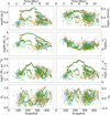 |
Fig. A.1 The three colours represent the axes along which the cube is projected. The colour scheme follows fig. 6. |
Appendix B 13CO(2-1) emission maps
In this section, we show a sequence of the 13CO(2-1) moment 0 maps for the GMC (i.e. the molecular gas complexes) as it evolves along with the dendrogram trunks (MCs). The MC obtained by projecting along three orthagonal axes (Sect. 3.1.2) are shown in Figures B.1–B.3. We also provide videos that represent all snapshots along the three projections as ancillary materials. This helps us to visualise the clouds and understand it’s structure at different evolutionary stages. Fig. B.1 shows the formation of MCs as small diffuse structures. Fig. B.2 shows a single (or a few) contour(s) that cover the entire emission in the viridis, representing most of the observed MCs. The filamentary, fractal, and complex nature of these structures is also visible in the emission maps. Fig. B.3 shows the MCs that are significantly impacted by stellar feedback processes. These lead to gas expulsion and dispersion, thus presenting the 13CO(2-1) as a 3D bubble. As more and more gas are dispersed, the number of MCs decreases. Some of these late MCs represent the early structures (Fig. B.1), with the difference that the early MCs have accompanying H2 gas. The absence of a molecular gas prevents the formation of MCs and ends the simulation.
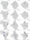 |
Fig. B.1 Moment 0 maps of 13CO(2-1) for different snapshots. The three columns represent the clouds projected along the x, y and z axes, respectively. The background grey scale represents H2 gas density with 13CO(2-1) emission overlaid as viridis maps, and coloured contours represent different MCs (dendrogram trunks), with red contours representing the largest MCs (R) in the cube. |
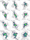 |
Fig. B.2 Moment 0 maps of 13CO(2-1) for different snapshots. The colours and symbols follow Fig. B.1. |
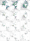 |
Fig. B.3 Moment 0 maps of 13CO(2-1) for different snapshots. The colours and symbols follow fig. B.1. |
Appendix C Inclusion of CO chemistry
We post-processed the STARFORGE simulations with UCLCHEM (Holdship et al. 2017) chemical code15 to estimate the abundance of CO (Sharda et al. in prep). However, due to computational cost, this has only been possible for three snapshots. Figures C.1 – C.3 show that although our fiducial approach slightly overestimates the 13CO emission, the data processing steps produce MCs of comparable size and morphology in both cases. This is further highlighted in Fig. C.4 & C.5, which show that both sets of MCs have similar properties in the same snapshots. The inclusion of chemistry might cause a small difference in the properties of our MCs and result in smaller MCs not being detectable. However, since we study the trends in the distribution of properties over time, we expect that these are not significantly influenced by the absence of CO chemistry.
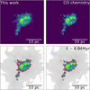 |
Fig. C.1 Comparison between the 13CO(2-1) ppv cube used in this work and created by including CO chemistry for snapshot 200 (4.94 Myr). The top rows show the RADMC-3D output and the bottom show the masked cubes with MCs (contours) overlayed on the 13CO(2-1) emission (viridis) and projected H2 density (grey scale) maps. |
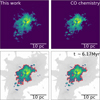 |
Fig. C.2 Comparison between the 13CO(2-1) ppv cube used in this work and created by including CO chemistry for snapshot 250 (6.17 Myr). The symbols and notations follow Fig. C.1. |
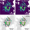 |
Fig. C.3 Comparison between the 13CO(2-1) ppv cube used in this work and created by including CO chemistry for snapshot 300 (7.41 Myr). The symbols and notations follow Fig. C.1. |
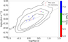 |
Fig. C.4 Size-linewidth relation (σv versus R) for our MCs (circles) and those created by including CO chemistry (plus). The MCs have been extracted from three ppv cubes in Figs. C.1–C.3. The symbols and notations are consistent with Fig. 8. |
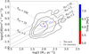 |
Fig. C.5 Scaling relation between |
![Mathematical equation: $\[\sigma_v^2 / R\]$](/articles/aa/full_html/2025/12/aa57095-25/aa57095-25-eq11.png)
Appendix D Hierarchical and isolated trunks
This section explains the reason for selecting only trunks that are branches as MCs, rather than including all trunks. In figure D.1, we show the distribution of properties for all dendrogram trunks. The results clearly demonstrate that only hierarchical trunks (branches) exhibit consistent trends in their properties as they evolve. In contrast, isolated trunks (leaves) have scattered distributions with no clear trends. This is likely because most of these isolated structures represent transient gas features that do not correspond to the fractal MCs seen in observations (Fig. B.1). Furthermore, the large sample of isolated trunks results in the average properties of the trunks (Fig. D.1, central line) that show no significant trends over time.
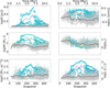 |
Fig. D.1 The cyan points represents the hierarchical trunks (branches) and grey points represents the isolated trunks (leaves). The coloured lines represents the average distribution of hierarchical trunks, with the colours following Fig. 5. The black line represents the average distribuion for isolated trunks. |
Appendix E Simulations with different initial turbulence
We perform our analysis on two other simulation sets. These have the same initial conditions as our fiducial runs, with the exception of initial turbulence. These are M2e4a1 and M2e4a4 with αvir = 1 and αvir = 4, respectively. Figs. E.1 & E.2 show the evolution of the MC properties for these two simulations, respectively. Although the GMC lifetime and the onset of different feedback mechanisms are different in the two simulations, they show a trend of increase in the MC properties representing actively growing MCs followed by a decrease in the properties due to MC dispersal by feedback. The morphology and fragementation trends of these MCs are consistent with the fiducial simulations.
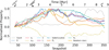 |
Fig. E.1 Simulation with αvir = 1. Properties of the clouds at various evolutionary stages. The R1 and R2 values represent the morphologies of the molecular gas complexes. The symbols and colours follow fig. 5 & 7. |
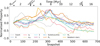 |
Fig. E.2 Simulation with αvir = 4. Properties of the clouds at various evolutionary stages. The symbols and colours follow fig. E.1. |
All Figures
|
Fig. 1 Left: synthetic integrated 13CO(2–1) emission map created with RADMC-3D. Right: same map but after convolution and with the noise of sigma = 0.2 ± 0.02 K. |
| In the text | |
|
Fig. 2 Comparison between the flux values for the noisy pixels from all the STARFORGE snapshots along all three projections and the complete SEDIGISM survey (13CO(2–1) emission). |
| In the text | |
|
Fig. 3 Comparison of MC properties from STARFORGE (left side violins) and SEDIGISM (right side violins). The properties are radius (R), velocity dispersion (σv), luminosity (L), virial parameter (αvir), and surface density (Σ). The horizontal dashed lines represent the quartiles of the distributions. |
| In the text | |
|
Fig. 4 Moment 0 maps of 13CO(2–1) at different evolutionary times. The background grey scale represents the H2 gas density with 13CO(2–1) emission overlaid as viridis maps (molecular gas complex), and the coloured contours represent different MCs (dendrogram trunks), with red contours representing the largest MCs (R) in the cube. The 13CO(2–1) maps for multiple snapshots along different projections are presented in Appendix B. |
| In the text | |
|
Fig. 5 Normalised medians of MC properties (log scales) as a function of time. The properties shown are radius (R), velocity dispersion (σv), molecular gas mass (M), virial parameter (αvir), surface mass density (Σ), and luminosity (L). The count refers to the total number of clouds in a time bin. The normalisation process included subtracting the initial value (first bin) of the property from it, and this was followed by a min-max standardisation. The symbols on the top represent the times at which outflows, photoionisation radiation, stellar winds, and supernovae begin in the simulation. |
| In the text | |
|
Fig. 6 Morphological analysis of the MCs (solid line) and molecular gas complexes (points) in different snapshots. R1 represents the degree of elongation, and R2 represents the degree of central concentration. The lines represent the R1 and R2 values for the MCs, and the scatter points represent the same for the molecular gas complexes, i.e. entire 13CO(2–1) emission in a snapshot, obtained using the projections along the three axes. The colour scheme is the same as in Fig. 3. |
| In the text | |
|
Fig. 7 Quantitative representation of MCs (counts), their substructures (dendrogram descendants), the newborn stars (age < 250 kyr), and the main-sequence stars more massive than 2M⊙ as a function of time. The values are normalised using a min–max standardisation. |
| In the text | |
|
Fig. 8 Size-linewidth relation (σv versus R) for our MCs (scatter points), colour-coded with respect to the time elapsed (in Myr) since the start of the simulation. The squares represent medians of distributions in ~1 Myr bins. The black contours represent the 1σ, 2σ, 3σ levels for the SEDIGISM clouds. The dashed line represents Larson’s first relation (Larson 1981; Solomon et al. 1987). |
| In the text | |
|
Fig. 9 Scaling relation between |
| In the text | |
|
Fig. A.1 The three colours represent the axes along which the cube is projected. The colour scheme follows fig. 6. |
| In the text | |
|
Fig. B.1 Moment 0 maps of 13CO(2-1) for different snapshots. The three columns represent the clouds projected along the x, y and z axes, respectively. The background grey scale represents H2 gas density with 13CO(2-1) emission overlaid as viridis maps, and coloured contours represent different MCs (dendrogram trunks), with red contours representing the largest MCs (R) in the cube. |
| In the text | |
|
Fig. B.2 Moment 0 maps of 13CO(2-1) for different snapshots. The colours and symbols follow Fig. B.1. |
| In the text | |
|
Fig. B.3 Moment 0 maps of 13CO(2-1) for different snapshots. The colours and symbols follow fig. B.1. |
| In the text | |
|
Fig. C.1 Comparison between the 13CO(2-1) ppv cube used in this work and created by including CO chemistry for snapshot 200 (4.94 Myr). The top rows show the RADMC-3D output and the bottom show the masked cubes with MCs (contours) overlayed on the 13CO(2-1) emission (viridis) and projected H2 density (grey scale) maps. |
| In the text | |
|
Fig. C.2 Comparison between the 13CO(2-1) ppv cube used in this work and created by including CO chemistry for snapshot 250 (6.17 Myr). The symbols and notations follow Fig. C.1. |
| In the text | |
|
Fig. C.3 Comparison between the 13CO(2-1) ppv cube used in this work and created by including CO chemistry for snapshot 300 (7.41 Myr). The symbols and notations follow Fig. C.1. |
| In the text | |
|
Fig. C.4 Size-linewidth relation (σv versus R) for our MCs (circles) and those created by including CO chemistry (plus). The MCs have been extracted from three ppv cubes in Figs. C.1–C.3. The symbols and notations are consistent with Fig. 8. |
| In the text | |
|
Fig. C.5 Scaling relation between |
| In the text | |
|
Fig. D.1 The cyan points represents the hierarchical trunks (branches) and grey points represents the isolated trunks (leaves). The coloured lines represents the average distribution of hierarchical trunks, with the colours following Fig. 5. The black line represents the average distribuion for isolated trunks. |
| In the text | |
|
Fig. E.1 Simulation with αvir = 1. Properties of the clouds at various evolutionary stages. The R1 and R2 values represent the morphologies of the molecular gas complexes. The symbols and colours follow fig. 5 & 7. |
| In the text | |
|
Fig. E.2 Simulation with αvir = 4. Properties of the clouds at various evolutionary stages. The symbols and colours follow fig. E.1. |
| In the text | |
Current usage metrics show cumulative count of Article Views (full-text article views including HTML views, PDF and ePub downloads, according to the available data) and Abstracts Views on Vision4Press platform.
Data correspond to usage on the plateform after 2015. The current usage metrics is available 48-96 hours after online publication and is updated daily on week days.
Initial download of the metrics may take a while.