| Issue |
A&A
Volume 704, December 2025
|
|
|---|---|---|
| Article Number | A252 | |
| Number of page(s) | 15 | |
| Section | Catalogs and data | |
| DOI | https://doi.org/10.1051/0004-6361/202557203 | |
| Published online | 18 December 2025 | |
Supplementing the 2MRS survey: The 2MZoA catalogue
Max-Planck-Institut für extraterrestrische Physik,
Gießenbachstraße 1,
85748
Garching,
Germany
★ Corresponding author: This email address is being protected from spambots. You need JavaScript enabled to view it.
Received:
11
September
2025
Accepted:
23
October
2025
Abstract
We present a homogeneous catalogue of verified 2MASX galaxies in high extinction areas that is complete to a Galactic extinction-corrected magnitude of Kso ≤ 11⋅m75. It covers the low Galactic latitudes (|b| ≤ 10⋅∘0), called Zone of Avoidance (ZoA), and areas of high foreground extinctions (E(B − V) > 0⋅m95) at higher latitudes. This catalogue supersedes the previously presented bright 2MZoA catalogue, which was only complete to Kso ≤ 11⋅m25. It fully complements the 2MASS Redshift Survey (2MRS) galaxy catalogue, which has the same magnitude limit but excludes high extinction regions. The combination of the two catalogues, the extended 2MRS or e2MRS, is a uniquely whole sky redshift survey of galaxies and forms a sound basis for studies of large-scale structures, cosmic flow fields, and extinction across the ZoA. The catalogue presented here comprises 6899 galaxies, with 6757 galaxies at low latitudes and 142 galaxies in highly obscured high-latitude areas. The completion rate in redshifts is almost 75%. The catalogue is complete up to star density levels of at least log N*/deg2 < 4.3, but the completion rate of the fainter part is affected by foreground extinction at all levels. This can be rectified by using a diameter-dependent extinction correction, which adds 605 highly obscured but apparently faint galaxies (with Kso > 11⋅m75 and Kso,d ≤ 11⋅m75) to the sample. This extended sample shows good completion rates with extinction up to at least AK < 1⋅m3. Omission of such a diameter-dependent extinction correction may lead to a biased flow field even at intermediate extinction values as found in the 2MRS survey. As in our previous investigations, we recommend a correction factor of f = 0.86 be applied to the extinction maps, and we find it to be independent of Galactic longitudes or latitudes.
Key words: catalogs / galaxies: general / galaxies: photometry / infrared: galaxies
© The Authors 2025
 Open Access article, published by EDP Sciences, under the terms of the Creative Commons Attribution License (https://creativecommons.org/licenses/by/4.0), which permits unrestricted use, distribution, and reproduction in any medium, provided the original work is properly cited.
This article is published in open access under the Subscribe to Open model.
Open Access funding provided by Max Planck Society.
1 Introduction
Our knowledge of the local Universe, that is, the local large-scale structures and related dynamics, is still incomplete due to the difficulties in finding and studying galaxies near the Galactic plane, the so-called Zone of Avoidance (ZoA). Dust extinction as well as star crowding severely hinder both the identification of galaxies (where different wavelengths are affected by different biases, e.g. Kraan-Korteweg & Lahav 2000 and references therein) as well as follow-up observations to obtain, for example, redshifts (e.g., Macri et al. 2019).
The ZoA is known to obscure and bisect major parts of dynamically important structures such as the Perseus-Pisces supercluster (Focardi et al. 1984; Chamaraux et al. 1990), the Great Attractor (Dressler et al. 1987; Kraan-Korteweg et al. 1996; Woudt et al. 2004), and the Local Void (Tully et al. 2008, 2019). Even nowadays, newly identified low-latitude structures are still being discovered, for example, the extended Vela supercluster (Kraan-Korteweg et al. 2017) at cz ~ 18 500 km s−1, contributing to the local bulk flow motion (e.g., Hudson et al. 2004; Springob et al. 2016).
While H I surveys are best at penetrating the foreground dust, they are mainly used to trace filaments through gas-rich spiral galaxies. In contrast, NIR surveys are better for obtaining a more comprehensive view of the local large-scale structures. Foreground extinction at these wavelengths is a lesser problem, and instead the detection of galaxies is more likely constrained by star crowding (e.g., Schröder et al. 2019, hereafter Paper I). The only truly all-sky NIR survey is the Two Micron All Sky Survey (2MASS; Skrutskie et al. 2006), which has a catalogue of extended sources, 2MASX (Jarrett 2004). A subset of this catalogue, restricted by Galactic latitude and foreground extinction, led to the 2MASS Redshift Survey (2MRS; Huchra et al. 2012).
2MASS is a comprehensive though shallow survey, and deeper NIR surveys covering only the ZoA exist, for example, the UKIDSS GPS (Galactic Plane Survey; Lucas et al. 2008), the Vista VVV (VISTA Variables in the Vía Lactea; Minniti et al. 2010) as well as VVVX (the extended VVV; Saito et al. 2024), and the DECam Plane Survey (Schlafly et al. 2018). With their higher resolution, they are ideal for detecting galaxies, but by-eye searches or even verification of automatically detected extended sources of such a data volume is not feasible anymore, and one needs to rely on other methods, such as machine learning (e.g., Daza-Perilla et al. 2023; Alonso et al. 2025).
To produce the extended 2MRS (e2MRS), which is the first nearly whole-sky redshift survey, our group has started to complement 2MRS by identifying 2MASX galaxies deep in the ZoA and measuring redshifts for them. As a pilot study, Paper I presents the 2MZoA catalogue of verified 2MASX galaxies down to an extinction-corrected magnitude limit of ![Mathematical equation: $\[K_{\mathrm{s}}^{\mathrm{o}}=11 ^{\mathrm{m}}_\cdot 25\]$](/articles/aa/full_html/2025/12/aa57203-25/aa57203-25-eq8.png) , which is complete up to star density levels of log N*/deg2 < 4.5, thus reducing the ZoA to 2.5–4% of the whole sky. Kraan-Korteweg et al. (2018) observed useful candidates with the Nançay Radio Telescope (NRT), resulting in 232 detections. An optical spectrographic survey is still ongoing. Schröder et al. (2021, hereafter Paper II) have used this sample to investigate the Galactic foreground extinction and recommend the extinction map presented by Planck Collaboration Int. XLVIII (2016) with a correction factor of f = 0.86 ± 0.01. In this paper, we present the extension of the 2MZoA catalogue down to an extinction-corrected magnitude limit of
, which is complete up to star density levels of log N*/deg2 < 4.5, thus reducing the ZoA to 2.5–4% of the whole sky. Kraan-Korteweg et al. (2018) observed useful candidates with the Nançay Radio Telescope (NRT), resulting in 232 detections. An optical spectrographic survey is still ongoing. Schröder et al. (2021, hereafter Paper II) have used this sample to investigate the Galactic foreground extinction and recommend the extinction map presented by Planck Collaboration Int. XLVIII (2016) with a correction factor of f = 0.86 ± 0.01. In this paper, we present the extension of the 2MZoA catalogue down to an extinction-corrected magnitude limit of ![Mathematical equation: $\[K_{\mathrm{s}}^{\mathrm{o}}=11^{\mathrm{m}}_\cdot 75\]$](/articles/aa/full_html/2025/12/aa57203-25/aa57203-25-eq9.png) so as to be fully complementary to 2MRS. Obtaining the missing redshifts will be more difficult, especially since many of the faintest galaxies are too obscured for optical spectroscopy and will require (N)IR spectroscopy or H I observations.
so as to be fully complementary to 2MRS. Obtaining the missing redshifts will be more difficult, especially since many of the faintest galaxies are too obscured for optical spectroscopy and will require (N)IR spectroscopy or H I observations.
This paper is organised as follows. In Sect. 2, we describe the sample, in Sect. 3 we present the catalogue, and in Sect. 4 we investigate its properties. Section 5 gives a discussion on differences and commonalities with Paper I and of various sub-samples. In Sect. 6 we revisit the investigation on Galactic foreground extinction from Paper II using the new sample. We finish with a summary in Sect. 7. Online tables and some plots are presented in the appendix.
2 The sample
Details of the sample selection and extraction can be found in Paper I. For convenience, we give a short summary and point out the differences due to the new selection criteria.
Our new magnitude limit is ![Mathematical equation: $\[K_{\mathrm{s}}^{\mathrm{o}} \leq 11^{\mathrm{m}}_\cdot 75\]$](/articles/aa/full_html/2025/12/aa57203-25/aa57203-25-eq10.png) . Contrary to the 2MRS sample and our bright 2MZoA sample, we decided to use a more suitable extinction map to correct for Galactic extinction, as investigated in Paper II. Instead of using the more common Schlegel et al. (1998) maps (hereafter SFD), we recommended the less biased Planck Collaboration Int. XLVIII (2016) maps, which were reduced using the generalised needlet internal linear combination (GNILC) component-separation method, hereafter called GN extinction. Furthermore, we applied a correction factor of f = 0.86 to the E(B − V) values, as also recommended in Paper II. For the 2MRS sample, the difference between the SFD and GN extinction corrections is considered negligible since they restrict their sample to areas where E(B − V) <
. Contrary to the 2MRS sample and our bright 2MZoA sample, we decided to use a more suitable extinction map to correct for Galactic extinction, as investigated in Paper II. Instead of using the more common Schlegel et al. (1998) maps (hereafter SFD), we recommended the less biased Planck Collaboration Int. XLVIII (2016) maps, which were reduced using the generalised needlet internal linear combination (GNILC) component-separation method, hereafter called GN extinction. Furthermore, we applied a correction factor of f = 0.86 to the E(B − V) values, as also recommended in Paper II. For the 2MRS sample, the difference between the SFD and GN extinction corrections is considered negligible since they restrict their sample to areas where E(B − V) < ![Mathematical equation: $\[1^{\mathrm{m}}_\cdot 0\]$](/articles/aa/full_html/2025/12/aa57203-25/aa57203-25-eq11.png) . The difference to the bright 2MZoA sample will be more noticeable, with new galaxies being included in the sample and others being excluded.
. The difference to the bright 2MZoA sample will be more noticeable, with new galaxies being included in the sample and others being excluded.
In addition, with the new redshift information and deep NIR images that have become available since Paper I, some of the object classifications have changed. We thus give a fully updated catalogue of all galaxies with ![Mathematical equation: $\[K_{\mathrm{s}}^{\mathrm{o}} \leq 11^{\mathrm{m}}_\cdot 75\]$](/articles/aa/full_html/2025/12/aa57203-25/aa57203-25-eq12.png) and include flags to indicate whether a galaxy is in the old and/or the new catalogue.
and include flags to indicate whether a galaxy is in the old and/or the new catalogue.
As in Paper I, we compiled two sub-samples:
ZOA sample: galaxies at |b| ≤ ![Mathematical equation: $\[10^{\circ}_\cdot 0\]$](/articles/aa/full_html/2025/12/aa57203-25/aa57203-25-eq13.png) at all Galactic longitudes;
at all Galactic longitudes;
EBV sample: all objects at |b| > ![Mathematical equation: $\[10^{\circ}_\cdot 0\]$](/articles/aa/full_html/2025/12/aa57203-25/aa57203-25-eq14.png) with E(B − V) >
with E(B − V) > ![Mathematical equation: $\[0^{\mathrm{m}}_\cdot 95\]$](/articles/aa/full_html/2025/12/aa57203-25/aa57203-25-eq15.png) .
.
The limit refers to SFD extinctions as to be as close to the 2MRS selection as possible; the overlap range has been chosen to cover any small variations in the actual calculation of E(B − V).
2.1 Sample extraction
From the online 2MASX catalogue1, we extracted all sources with the sub-sample selection criteria as well as the default SQL constraints given in the webform. The resulting sample is the same as in Paper I. Next, we applied the GN extinction correction to extract the magnitude-limited sample of objects, using the following extinction conversion factors (Fitzpatrick 1999): Aλ/AB = 0.208, 0.128, 0.087 for J-, H-, and Ks-band, repetitively. Table 1 lists the numbers of objects in the respective samples, ZOA and EBV, for the original catalogue (Paper I) and for the present catalogue. For better comparison, we also give numbers for the bright sample (![Mathematical equation: $\[K_{\mathrm{s}}^{\mathrm{o}} \leq 11^{\mathrm{m}}_\cdot 25\]$](/articles/aa/full_html/2025/12/aa57203-25/aa57203-25-eq16.png) ) and the faint sample (
) and the faint sample (![Mathematical equation: $\[11^{\mathrm{m}}_\cdot25<K_{\mathrm{s}}^{\mathrm{o}} \leq 11^{\mathrm{m}}_\cdot75\]$](/articles/aa/full_html/2025/12/aa57203-25/aa57203-25-eq17.png) ) separately.
) separately.
All 2MASX catalogue entries obeying the selection criteria have been inspected visually on optical and NIR images and given a flag according to the confidence we have that they are galaxies. Compared with Paper I, the availability of deep NIR survey images has increased2, with 89% of the ZOA objects and 76% of the EBV objects now covered.
As in Paper I, we extracted redshift information from online data bases and literature, which also helped with the classification (see Appendix A for details). Finally, we visually estimated galaxy types regarding the presence or absence of a disc (mainly in preparation for H I follow-up observation); the B- and R-band images proved most useful for low-extinction galaxies, while the deep K-band images were most helpful in high-extinction areas. In addition to Paper I, we flag known and suspected active galaxies (AGNs) since these often have a redder colour. We also revisited the extinction flag and re-evaluated those for the bright sample.
As a result, we have a total of 6899 galaxies, with 6757 in the ZOA sample and 142 in the EBV sample. In addition, there are nine galaxy candidates, all in the ZOA sample. The differences to Paper I in the bright sample source numbers are mainly due to the newly applied extinction correction factor (which reduces the extinction correction, resulting in fainter corrected magnitudes) and, to a smaller degree, due to differences between the SFD and GN extinction values.
Object samples at different stages during extraction.
2.2 Sub-samples and supplementary samples
In the catalogue, we give flags for various sample definitions for convenience. As already indicated in Table 1, we can define a bright and a full sample (with ![Mathematical equation: $\[K_{\mathrm{s}}^{\mathrm{o}} \leq 11^{\mathrm{m}}_\cdot 25\]$](/articles/aa/full_html/2025/12/aa57203-25/aa57203-25-eq18.png) and
and ![Mathematical equation: $\[K_{\mathrm{s}}^{\mathrm{o}} \leq 11^{\mathrm{m}}_\cdot 75\]$](/articles/aa/full_html/2025/12/aa57203-25/aa57203-25-eq19.png) , respectively). For easier comparison with Paper I, we give an ‘original sample’ flag based on SFD extinction correction with no correction factor (note that the number of galaxies in this sample still differs from Paper I due to changes in galaxy class settings). We also give a flag for the full sample but with no correction factor applied to the E(B − V) values, which makes it easier to investigate this factor further if there is a need.
, respectively). For easier comparison with Paper I, we give an ‘original sample’ flag based on SFD extinction correction with no correction factor (note that the number of galaxies in this sample still differs from Paper I due to changes in galaxy class settings). We also give a flag for the full sample but with no correction factor applied to the E(B − V) values, which makes it easier to investigate this factor further if there is a need.
We list the sample flags with their definitions as well as the numbers of objects and of galaxies in Table 2. Note that the sample flags do not distinguish between the ZOA and EBV samples since these can be simply selected by Galactic latitude.
As mentioned in Paper I, the isophotal diameter of a galaxy is also affected by extinction, and an additional, diameter-dependent, extinction correction should be applied. This correction, however, has large uncertainties and is best applied to the individual galaxy photometry by extrapolating the radial brightness curves (Riad et al. 2010). We therefore do not use it in our recommended sample. Instead, we have compiled an extended sample based on these corrections, which will help in understanding the effects of applying such a correction on sample size and characteristics. We give two such sample flags: One is based on the faint limit ![Mathematical equation: $\[K_{\mathrm{s}}^{\mathrm{o}, \mathrm{d}} \leq 11^{\mathrm{m}}_\cdot 75\]$](/articles/aa/full_html/2025/12/aa57203-25/aa57203-25-eq26.png) , with the GN extinction correction and a factor of 0.86 applied, and the other refers to the sample presented in Paper I and is based on the SFD extinctions (
, with the GN extinction correction and a factor of 0.86 applied, and the other refers to the sample presented in Paper I and is based on the SFD extinctions (![Mathematical equation: $\[K_{\mathrm{s}}^{\mathrm{o}, \mathrm{d}} \leq 11^{\mathrm{m}}_\cdot 25\]$](/articles/aa/full_html/2025/12/aa57203-25/aa57203-25-eq27.png) ), with a correction factor of f = 0.83 applied.
), with a correction factor of f = 0.83 applied.
Various sample flags.
3 The catalogue
The catalogue with a total of 10 960 ZOA and 616 EBV objects is available online at CDS; a few example rows are listed in Table A.1. It supersedes the catalogues given in Paper I. The table comes in two sections: (a) full sample as per our selection criteria and (b) a supplementary sample for objects that obey the limit ![Mathematical equation: $\[K_{\mathrm{s}}^{\mathrm{o}, \mathrm{d}} \leq 11^{\mathrm{m}}_\cdot 75\]$](/articles/aa/full_html/2025/12/aa57203-25/aa57203-25-eq28.png) but not
but not ![Mathematical equation: $\[K_{\mathrm{s}}^{\mathrm{o}} \leq 11^{\mathrm{m}}_\cdot 75\]$](/articles/aa/full_html/2025/12/aa57203-25/aa57203-25-eq29.png) when a diameter-dependent extinction correction is applied3. Columns are the same as in Paper I except for a different suite of sample flags, listed in Col. 7, and an updated object flag in Col 6, which now includes an indicator for AGNs. We also added the best velocity measurement found in the literature and include detailed flags separately for optical and H I velocities in Col. 10.
when a diameter-dependent extinction correction is applied3. Columns are the same as in Paper I except for a different suite of sample flags, listed in Col. 7, and an updated object flag in Col 6, which now includes an indicator for AGNs. We also added the best velocity measurement found in the literature and include detailed flags separately for optical and H I velocities in Col. 10.
The columns in the catalogue are as follows:
Col. 1: ID: 2MASX catalogue identification number (based on J2000.0 coordinates).
Col. 2a and 2b: galactic coordinates: longitude l and latitude b, in degrees.
Col. 3: extinction: E(B − V) value derived from the GNILC Planck maps (Planck Collaboration Int. XLVIII 2016), in magnitudes.
Col. 4: object class: 1 = obvious galaxy, 2 = galaxy, 3 = probable galaxy, 4 = possible galaxy, 5 = unknown, 6 = lower likelihood for galaxy, 7 = unlikely galaxy, 8 = no galaxy, 9 = obviously not a galaxy.
Col. 5: object offset flag: ‘o’ stands for coordinates that are offset from the centre of the object, and ‘e’ stands for a detection near the edge of an image (at an offset position from the object centre; the properly centred object is detected on the adjacent image).
Col. 6: object flag: ‘p’ stands for planetary nebula (PN), ‘q’ indicates a QSO/AGN, and ‘b’ stands for blazar; tentative classifications are indicated by a question mark.
-
Col. 7: sample flags in the following order:
- (a)
fgal: Galaxy flag: ‘g’ denotes a galaxy (object classes 1–4), and ‘p’ stands for galaxy candidates (class 5);
- (b)
fsam: Full sample (
![Mathematical equation: $\[K_{\mathrm{s}}^{\mathrm{o}} \leq 11^{\mathrm{m}}_\cdot 75\]$](/articles/aa/full_html/2025/12/aa57203-25/aa57203-25-eq30.png) , GN extinction correction, f = 0.86);
, GN extinction correction, f = 0.86); - (c)
forig: Bright sample as in Paper I (
![Mathematical equation: $\[K_{\mathrm{s}}^{\mathrm{o}} \leq 11^{\mathrm{m}}_\cdot 25\]$](/articles/aa/full_html/2025/12/aa57203-25/aa57203-25-eq31.png) , SFD extinction correction, no correction factor);
, SFD extinction correction, no correction factor); - (d)
fbr: Bright sample, this paper, for comparison with Paper I (
![Mathematical equation: $\[K_{\mathrm{s}}^{\mathrm{o}} \leq 11^{\mathrm{m}}_\cdot 25\]$](/articles/aa/full_html/2025/12/aa57203-25/aa57203-25-eq32.png) , GN extinction correction, f = 0.86);
, GN extinction correction, f = 0.86); - (e)
fno–f: Full sample with no correction factor applied (
![Mathematical equation: $\[K_{\mathrm{s}}^{\mathrm{o}} \leq 11^{\mathrm{m}}_\cdot 75\]$](/articles/aa/full_html/2025/12/aa57203-25/aa57203-25-eq33.png) , GN extinction correction, f = 1.0);
, GN extinction correction, f = 1.0); - (f)
fext: Extended sample, with diameter-dependent extinction correction applied (
![Mathematical equation: $\[K_{\mathrm{s}}^{\mathrm{o}, \mathrm{d}} \leq 11^{\mathrm{m}}_\cdot 75\]$](/articles/aa/full_html/2025/12/aa57203-25/aa57203-25-eq34.png) , GN extinction correction, f = 0.86);
, GN extinction correction, f = 0.86); - (g)
fext–orig: Extended sample as in Paper I, with diameter-dependent extinction correction (
![Mathematical equation: $\[K_{\mathrm{s}}^{\mathrm{o}, \mathrm{d}} \leq 11^{\mathrm{m}}_\cdot 75\]$](/articles/aa/full_html/2025/12/aa57203-25/aa57203-25-eq35.png) , SFD extinction correction, f = 0.83).
, SFD extinction correction, f = 0.83).
- (a)
Col. 8: galaxy disc type: ‘D1’ means an obviously visible disc and/or spiral arms, ‘D2’ stands for a noticeable disc, ‘D3’ for a possible disc, and ‘D4’ stands for no disc noticeable. Where it was not possible to tell (likely due to adjacent or superimposed stars or very high extinction) we give a flag ‘n’.
Col. 9: 2MRS flags: ‘c’ stands for an entry in the main catalogue, and ‘e’ for the extra catalogue (that is, outside the 2MRS selection criteria). For the sub-catalogues4 we give: ‘cf’ for an entry in the flg catalogue (affected by nearby stars, but not severely), ‘cp’ for an entry in the flr catalogue (severely affected by nearby stars), ‘ca’ and ‘ea’ are objects that have been reprocessed and are both in the rep as well as add catalogues (in the latter case with new IDs and photometry, not listed by us), ‘cr’ and ‘er’ are objects rejected as galaxies and which can be found in the rej catalogues, ‘cn’ and ‘en’ are objects that have no redshifts yet and are listed in the nocz catalogues.
Cols. 10a–10c: velocity flags ‘vo’, ‘vh’ and ‘vtot’: ‘o’ stands for an optical measurement and ‘h’ for H I velocity; a colon indicates an uncertain measurement and a question mark stands for a questionable measurement, object ID or target (in particular for H I: a radio telescope’s large beam size may include nearby galaxies), or an uncertain detection (often with a low signal-to-noise ratio); ‘g’ indicates a velocity measurement of a Galactic source5. Square brackets in Cols. 10a and 10b indicate a non-accepted velocity (due to questionable ID or measurement), and normal brackets in Col. 10c indicate not yet published measurements. In a few cases, though published values exist we prefer unpublished measurements (e.g. when they have better errors).
Col. 11: deep NIR image flag: ‘U’ indicates a UKIDSS image for this object, ‘H’ stands for a UHS, and ‘V’ stands for VISTA.
Col. 12: photometry flag: ‘O’ indicates off-centre coordinates (cf. Col. 5), ‘A’, ‘P’ and ‘F’ refer to the respective 2MRS flag (cf. Col. 9), and ‘C’ denotes improved photometry exists in John Huchra’s original list (see Paper I for details).
Col. 13: extinction flag (see Paper I): ‘e’ stands for a likely wrong extinction value, either due to small-scale variations or a non-removed FIR point source, ‘e?’ denotes a possible wrong extinction value. Note that these have been updated since Paper I.
Col. 14: 2MASX magnitude K20: isophotal Ks-band magnitude measured within the Ks-band 20 mag arcsec−2 isophotal elliptical aperture (in magnitudes).
Cols. 15 and 16: 2MASX colours (H − Ks) and (J − Ks): isophotal colours measured within the Ks-band 20 mag arcsec−2 isophotal elliptical aperture (in magnitudes).
Col. 17: 2MASX flag vc: the visual verification score of a source.
Col. 18: 2MASX object size a: the major diameter of the object, which is twice the 2MASX Ks-band 20 mag arcsec−2 isophotal elliptical aperture semi-major axis r_k20fe (in arcseconds).
Col. 19: 2MASX axis ratio b/a: minor-to-major axis ratio fit to the 3σ super-co-added isophote, sup_ba. Single-precision entries are given in cases where the 2MASX parameter sup_ba is not determined; these values were estimated from the axial ratios available in the different passbands.
Col. 20: 2MASX stellar density: co-added logarithm of the number of stars (Ks < 14 mag) per square degree around the object.
Cols. 21–23: magnitude
![Mathematical equation: $\[K_{\mathrm{s}}^{\mathrm{o}}\]$](/articles/aa/full_html/2025/12/aa57203-25/aa57203-25-eq36.png) and colours (H − Ks)o and (J − Ks)o corrected for foreground extinction (Col. 3) using a correction factor of 0.86 (in magnitudes).
and colours (H − Ks)o and (J − Ks)o corrected for foreground extinction (Col. 3) using a correction factor of 0.86 (in magnitudes).Col. 24: extinction in the Ks-band AK: calculated from E(B − V) in Col. 3 and applying a correction factor of 0.86 (in magnitudes).
Col. 25: extinction corrected major diameter ad according to Riad et al. (2010) using E(B − V) from Col. 4 with the correction factor of 0.86; only given for objects classified as galaxies (in arcseconds).
Col. 26: extinction corrected magnitude
![Mathematical equation: $\[K_{\mathrm{s}}^{\mathrm{o}, \mathrm{d}}\]$](/articles/aa/full_html/2025/12/aa57203-25/aa57203-25-eq37.png) corrected according to Riad et al. (2010) using E(B − V) from Col. 3 with the correction factor of 0.86; only given for objects classified as galaxies (in magnitudes).
corrected according to Riad et al. (2010) using E(B − V) from Col. 3 with the correction factor of 0.86; only given for objects classified as galaxies (in magnitudes).Cols. 27 and 28: adopted radial, heliocentric velocity with error and reference according to the vtot flag in Col. 10c. If the measurement is not yet published, we quote a token reference and do not give the velocity here.
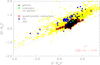 |
Fig. 1 2MASS extinction-corrected colour–colour plot, (H − Ks)o versus (J − Ks)o. A reddening vector, representing the mean of the sample shown, is indicated by a red arrow in the bottom right corner. The reddening path for objects within the intrinsic colour range of galaxies is indicated with two parallel dashed lines. |
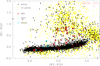 |
Fig. 2 WISE extinction-corrected colour–colour plot, (W1 − W2)o versus (W2 − W3)o for the full sample. A reddening vector, representing the mean of the sample shown, is indicated by a red arrow in the top right corner. Open circles mark active galaxies as labelled. |
4 Properties of the catalogue
We have thoroughly discussed the properties of the bright 2MZoA catalogue in Paper I, and most of it also applies to the full sample. In the following, we show some updated plots and statistics. A sky map with the distribution of the samples are shown in the appendix; it is not qualitatively different from the maps shown in Paper I.
Figure 1 shows the colour–colour plot with objects classified as galaxies in black and non-galaxies in yellow; the few galaxy candidates (objects of unknown classification, class 5) are shown in green. Clearly offset in (H − Ks)o colour are PNe, which are shown as blue dots (where open circles indicate possible PNe). The reddening path for the intrinsic colour range occupied by the bulk of the galaxies is shown by the two dashed lines. Galaxies with wrong Galactic extinction values scatter along this path. This is confirmed by the distribution of the red circles, which mark galaxies where we stated a questionable extinction based on visually obvious variations across the images (extinction flag e). Galaxies lying outside the reddening path are likely to be affected by starlight in the photometry aperture.
For the WISE colour–colour plot (Fig. 2), we use the aperture 1 (![Mathematical equation: $\[5^{\prime \prime}_\cdot 5\]$](/articles/aa/full_html/2025/12/aa57203-25/aa57203-25-eq38.png) ) magnitudes of the ALLWISE catalogue, corrected for foreground extinction, as in Paper I. Spiral galaxies are located more to the right, and ellipticals are predominantly found to the left (see Figure 26 in Jarrett et al. 2011), while active and intensely star forming galaxies are separated in (W1 − W2), top. We marked all AGNs listed in the literature with red circles and blazars with cyan circles; possible AGNs (based on their colour and visual appearance) are marked with green circles.
) magnitudes of the ALLWISE catalogue, corrected for foreground extinction, as in Paper I. Spiral galaxies are located more to the right, and ellipticals are predominantly found to the left (see Figure 26 in Jarrett et al. 2011), while active and intensely star forming galaxies are separated in (W1 − W2), top. We marked all AGNs listed in the literature with red circles and blazars with cyan circles; possible AGNs (based on their colour and visual appearance) are marked with green circles.
The completeness of a sample of galaxies can be shown in various ways. Figure 3 shows histograms of source counts as a function of Galactic latitude and longitude. While the galaxy counts (red) show a small dip near the Galactic plane (Panel a), the distribution of all sources (in blue) shows a clear peak, emphasising the need for visual inspection to identify non-Galaxian extended objects in the 2MASX catalogue for the inner ZoA (|b| < 5°). For comparison, the black line represents the average galaxy density outside of the ZoA, which is 1.212 galaxies/sq. deg (black line) based on source counts of the 2MASX catalogue with |b| > 30° and K20 ≤ ![Mathematical equation: $\[11^{\mathrm{m}}_\cdot75\]$](/articles/aa/full_html/2025/12/aa57203-25/aa57203-25-eq39.png) . Panels b and c show the semi-circles towards the anti-centre and the Galactic bulge, respectively. The dip in galaxy counts disappears in the anticentre direction but is greatly pronounced towards the Galactic bulge. As already noted in Paper I, the dip towards the Galactic Bulge indicates a breakdown in galaxy recognition of the 2MASX survey mainly due to star crowding.
. Panels b and c show the semi-circles towards the anti-centre and the Galactic bulge, respectively. The dip in galaxy counts disappears in the anticentre direction but is greatly pronounced towards the Galactic bulge. As already noted in Paper I, the dip towards the Galactic Bulge indicates a breakdown in galaxy recognition of the 2MASX survey mainly due to star crowding.
We can also show completeness levels as a function of stellar densities and extinction, see Fig. 4 top and bottom panel, respectively. For the extinction plot we only used areas with stellar densities log N*/deg2 < 4.5 (to avoid a selection bias since both high extinction and high stellar density occur in similar areas). The number densities are highly affected by low number statistics for AK ≳ ![Mathematical equation: $\[1^{\mathrm{m}}_\cdot 0\]$](/articles/aa/full_html/2025/12/aa57203-25/aa57203-25-eq40.png) . Due to the small area covered by our sample, the numbers are also subject to cosmic variance. However, we can make two broad statements: Extinction seems to affect galaxy counts at all levels, and the effect of stellar density is negligible up to log N*/deg2 ~ 4.3 and becomes severe at log N*/deg2 > 4.5.
. Due to the small area covered by our sample, the numbers are also subject to cosmic variance. However, we can make two broad statements: Extinction seems to affect galaxy counts at all levels, and the effect of stellar density is negligible up to log N*/deg2 ~ 4.3 and becomes severe at log N*/deg2 > 4.5.
Table 3 gives the statistics on some of the parameters in the ZOA and EBV catalogues. For better comparison, we give percentages with respect to all galaxies in the respective sample, with the total numbers listed at the bottom. Regarding the disc parameter, we find that over 80% of all galaxies show a disc, while only around 4% have no indication of one. Extinction flags were set for ~20% of galaxies in the ZOA sample, with a much higher fraction of ~65% for the EBV sample. The latter is expected since the EBV sample covers only high extinction areas.
As to redshift information, more than 70% of the sample galaxies have redshift measurements, the majority of which are optical. We distinguish between optical and H I measurements, and also whether the velocity information has been published6 (vlit). We separately list cases where it appears questionable that the measured redshift belongs to the targeted galaxy (indicated with a question mark). This mainly concerns H I measurements, where the often very large beam size can include other galaxies close by. Though we give such velocities in our catalogue, they have been flagged in Col. 10c with a question mark and are ignored in our analysis.
We also flagged all objects that appear in the 2MRS catalogues (Huchra et al. 2012; Macri et al. 2019), though the percentages given here relate only to objects classified by us as galaxies. Furthermore, we noted but not extracted photometric redshift information in the literature7. Since photometric redshifts have large uncertainties (and can be affected by stars in the aperture), we do not find them useful for our, predominantly local, sample. Finally, we noted a number of possible H I detections, which need confirmation before we can make use of them.
Figure 5 shows the histograms for the (J − Ks)o and (H − Ks)o colours (green lines). In Paper I we had found that there is a dependence on stellar density. We re-analysed the relationship for the new sample and found slightly improved dependencies:
![Mathematical equation: $\[\left(J-K_{\mathrm{S}}\right)^{\mathrm{o}}=(-0.064 \pm 0.007) \cdot \log~ N_* / \operatorname{deg}^2+~(1.244 \pm 0.027)\]$](/articles/aa/full_html/2025/12/aa57203-25/aa57203-25-eq41.png)
and
![Mathematical equation: $\[\left(H-K_{\mathrm{S}}\right)^{\mathrm{o}}=(-0.039 \pm 0.005) \cdot \log~ N_* / \operatorname{deg}^2+~(0.453 \pm 0.020).\]$](/articles/aa/full_html/2025/12/aa57203-25/aa57203-25-eq42.png)
The magenta-coloured histogram shows the accordingly corrected colours, and Table 4 gives the statistics of the colours with and without the correction. As in Paper I, we also show the histograms for galaxies outside the ZoA for comparison (yellow). Contrary to Paper I, we chose a higher latitude cut-off to make sure that extinction will not affect the (uncorrected) colours. With cuts at |b| > 30° and Ks < ![Mathematical equation: $\[11^{\mathrm{m}}_\cdot 75\]$](/articles/aa/full_html/2025/12/aa57203-25/aa57203-25-eq43.png) , the high-latitude sample comprises 25 007 galaxies. As described in Paper I in more detail, we formed 16 sub-samples containing each about 3000 galaxies to test for cosmic variance. The yellow histograms show the mean normalised counts with error bars based on the standard deviation of the 16 sub-samples. The mean as well as the range of values for the 16 high-latitude sub-samples are also given in Table 4. Since colours are affected by k-correction (noticeable as an extended red tail in the histograms), we prefer the median to the mean. There is good agreement between the high and low latitude samples if we apply the stellar density correction to our sample.
, the high-latitude sample comprises 25 007 galaxies. As described in Paper I in more detail, we formed 16 sub-samples containing each about 3000 galaxies to test for cosmic variance. The yellow histograms show the mean normalised counts with error bars based on the standard deviation of the 16 sub-samples. The mean as well as the range of values for the 16 high-latitude sub-samples are also given in Table 4. Since colours are affected by k-correction (noticeable as an extended red tail in the histograms), we prefer the median to the mean. There is good agreement between the high and low latitude samples if we apply the stellar density correction to our sample.
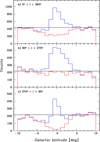 |
Fig. 3 Histograms of objects in the ZOA sample as a function of Galactic latitude for all objects (blue) and for galaxies only (red). The black line represents the average 2MASX galaxy count outside the ZoA. Panel a: for all Galactic longitudes; panel b for the semi-circle towards the anti-centre region; panel c for the semi-circle towards the bulge. |
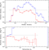 |
Fig. 4 Histograms of the number density of all ZOA sample objects (blue) and galaxies only (red) as a function of stellar density (top panel) and Galactic extinction AK (bottom panel; only regions with log N*/deg2 ≤ 4.5 were used). The error bars indicate Poissonian errors per bin. The dotted black lines represent the average 2MASX bright galaxy number density outside of the ZoA. |
Statistics on some parameters for both samples.
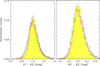 |
Fig. 5 Normalised histograms of 2MASX colours (J − Ks)o (left) and (H − Ks)o (right). Green histograms are the full sample and the magenta histograms show colours corrected for stellar densities. the yellow-filled histograms represent the average high Galactic latitude sample. |
5 Sample comparisons
There are two major differences to Paper I:
(1) As explained above, we use an improved extinction correction, which changes the composition of the sample for ![Mathematical equation: $\[K_{\mathrm{s}}^{\mathrm{o}} \leq11^{\mathrm{m}}_\cdot 25\]$](/articles/aa/full_html/2025/12/aa57203-25/aa57203-25-eq44.png) . In addition, with new deep NIR images and velocity information, some objects have a changed object class and have thus entered or left the bright galaxy sample.
. In addition, with new deep NIR images and velocity information, some objects have a changed object class and have thus entered or left the bright galaxy sample.
(2) By extending the magnitude limit from ![Mathematical equation: $\[11^{\mathrm{m}}_\cdot 25\]$](/articles/aa/full_html/2025/12/aa57203-25/aa57203-25-eq45.png) to
to ![Mathematical equation: $\[11^{\mathrm{m}}_\cdot 75\]$](/articles/aa/full_html/2025/12/aa57203-25/aa57203-25-eq46.png) , the qualitative composition of the sample likely has changed since fainter galaxies are either smaller or more distant.
, the qualitative composition of the sample likely has changed since fainter galaxies are either smaller or more distant.
5.1 Comparison with Paper I
We can make a direct comparison with Paper I by applying the same magnitude limit ![Mathematical equation: $\[11^{\mathrm{m}}_\cdot 25\]$](/articles/aa/full_html/2025/12/aa57203-25/aa57203-25-eq47.png) to our here presented sample. First of all, the new sample is smaller since we apply a correction factor smaller than one to the extinction values, resulting in fainter magnitudes, which affects the sample size. For clarity, we also compared the effects of applying the SFD corrections (with and without a correction factor) instead of the GN extinction. The top section of Table 5 gives the various sample sizes.
to our here presented sample. First of all, the new sample is smaller since we apply a correction factor smaller than one to the extinction values, resulting in fainter magnitudes, which affects the sample size. For clarity, we also compared the effects of applying the SFD corrections (with and without a correction factor) instead of the GN extinction. The top section of Table 5 gives the various sample sizes.
While for each galaxy the GN extinction value may be smaller or larger than the SFD value, the overall effect on the sample is that we lose more objects than we gain. However, this seems to be only the case for the non-galaxies (ΔN = 405 and 452 for the ZOA sample, depending on whether f was applied or not, respectively), while the differences in the galaxy samples are negligible (ΔN = −37 and −10, respectively). We therefore do not expect (and have not found) any qualitative differences with the discussion in Paper I regarding the bright galaxy sample.
5.2 Bright versus faint
To investigate qualitative differences between bright and faint galaxies, we divided our sample into the three sub-samples bright (S1), medium (S2) and faint (S3), with ![Mathematical equation: $\[K_{\mathrm{s}}^{\mathrm{o}} \leq 11^{\mathrm{m}}_\cdot 25\]$](/articles/aa/full_html/2025/12/aa57203-25/aa57203-25-eq48.png) ,
, ![Mathematical equation: $\[11^{\mathrm{m}}_\cdot 25<K_{\mathrm{s}}^{\mathrm{o}} \leq 11^{\mathrm{m}}_\cdot 50\]$](/articles/aa/full_html/2025/12/aa57203-25/aa57203-25-eq49.png) and
and ![Mathematical equation: $\[11^{\mathrm{m}}_\cdot 50<K_{\mathrm{s}}^{\mathrm{o}} \leq 11^{\mathrm{m}}_\cdot 75\]$](/articles/aa/full_html/2025/12/aa57203-25/aa57203-25-eq50.png) , respectively. Sample sizes are given in the second part of Table 5.
, respectively. Sample sizes are given in the second part of Table 5.
First of all, we show the distribution of the three sub-samples across Galactic latitudes in Fig. 6 for all sources (left panel), galaxies (middle panel) and the ratio of galaxies versus all sources (right panel). While the dip in galaxy numbers seen in Fig. 3 around the Galactic plane persists (and varies similarly with longitude, not shown), only the S1 sample (red) shows a clear peak of non-galaxies near the plane. To investigate this further, we show the ![Mathematical equation: $\[K_{\mathrm{s}}^{\mathrm{o}}\]$](/articles/aa/full_html/2025/12/aa57203-25/aa57203-25-eq51.png) -band histogram in Fig. 7 (left panel) for non-galaxies in black and galaxies in red. While the galaxies show the typical exponential luminosity function, the number counts of non-galaxies increases much slower (almost but not quite linearly). It should be noted that the non-galaxies are mainly Galactic nebulae or parts thereof, with some artefacts and stars or batches of faint stars added to the mix. Due to their size and the overestimation of foreground extinction, the detections of the nebulae are usually bright, and it is therefore obvious that the fainter samples show much less contamination. To emphasise this, we show the histogram of diameters (right hand panel in Fig. 7). At large diameters the non-galaxies dominate as expected. Non-galaxies also dominate at the smallest diameters, which is likely due to the spurious detection of stars.
-band histogram in Fig. 7 (left panel) for non-galaxies in black and galaxies in red. While the galaxies show the typical exponential luminosity function, the number counts of non-galaxies increases much slower (almost but not quite linearly). It should be noted that the non-galaxies are mainly Galactic nebulae or parts thereof, with some artefacts and stars or batches of faint stars added to the mix. Due to their size and the overestimation of foreground extinction, the detections of the nebulae are usually bright, and it is therefore obvious that the fainter samples show much less contamination. To emphasise this, we show the histogram of diameters (right hand panel in Fig. 7). At large diameters the non-galaxies dominate as expected. Non-galaxies also dominate at the smallest diameters, which is likely due to the spurious detection of stars.
Figure 8 compares the samples regarding stellar density (left panel) and extinction (right panel). All three samples show stable number densities for stellar densities of log N*/deg2 ≥ 3.4, the sharp cut-off at log N*/deg2 ≥ 4.5 known from Paper I (and here visible for S1) is less pronounced for the fainter samples with a reduced limit of log N*/deg2 ~ 4.4, indicating that stellar densities affect more the detection of smaller and fainter galaxies. The extinction also affects more strongly the two fainter samples. Due to the limit in extinction-corrected magnitude, the maximum AK value drops from ![Mathematical equation: $\[2^{\mathrm{m}}_\cdot 1\]$](/articles/aa/full_html/2025/12/aa57203-25/aa57203-25-eq57.png) to
to ![Mathematical equation: $\[1^{\mathrm{m}}_\cdot 7\]$](/articles/aa/full_html/2025/12/aa57203-25/aa57203-25-eq58.png) to
to ![Mathematical equation: $\[1^{\mathrm{m}}_\cdot 3\]$](/articles/aa/full_html/2025/12/aa57203-25/aa57203-25-eq59.png) , respectively. The faintest sample S3 (magenta) shows a decrease even in the first three bins (
, respectively. The faintest sample S3 (magenta) shows a decrease even in the first three bins (![Mathematical equation: $\[A_{\mathrm{K}}<0^{\mathrm{m}}_\cdot6\]$](/articles/aa/full_html/2025/12/aa57203-25/aa57203-25-eq60.png) ) and both S2 and S3 show a gradual decrease beyond
) and both S2 and S3 show a gradual decrease beyond ![Mathematical equation: $\[A_{\mathrm{K}}<0^{\mathrm{m}}_\cdot6\]$](/articles/aa/full_html/2025/12/aa57203-25/aa57203-25-eq61.png) . We conclude that the faintest sample is not complete at any extinction level.
. We conclude that the faintest sample is not complete at any extinction level.
Statistics of the parameters disc class, extinction flag and availability of redshift measurement information are presented in Table 6, similarly to Table 3. While the disc class parameter shows the increasing difficulties to classify fainter (and smaller) galaxies, the determination of the extinction flag is independent of the kind of detected galaxy. There is also a marked (and expected) decrease in redshift measurements for the fainter samples, especially in H I measurements. This is partly because mostly bright and large galaxies are targeted in H I surveys. In addition, the sensitivity decreases rapidly with distance so that most blind H I surveys do not go much beyond v = 10 000 km s−1. However, this will change with the new generation of radio telescopes such as MeerKAT, ASKAP and, eventually, the SKA.
Representation in the 2MRS catalogue is stable across all samples as expected since we chose the same magnitude limit. The inclusion in the 2MRS extra catalogue decreases for the fainter samples since galaxies were not systematically included in this catalogue but only through availability of redshift measurements in the literature.
Finally, we present the mean and median colours for the various samples in Table 7. It is obvious that the colours become redder for the fainter samples, which is also the case for the high-latitude samples and thus not caused by the higher extinctions. Instead, such a shift is expected since we have not applied a k-correction. A similar shift has been noted for the bright sample in Paper II (see their Figure 8) where we compared (uncorrected) colours of galaxies in various redshift bins.
Statistics on 2MASX colours of various samples.
Various samples with different ![Mathematical equation: $\[K_{\mathrm{s}}^{\mathrm{o}}\]$](/articles/aa/full_html/2025/12/aa57203-25/aa57203-25-eq52.png) band limits.
band limits.
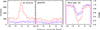 |
Fig. 6 Histograms of objects in the ZOA samples with Galactic latitude: all objects (left), galaxies (middle), and the fraction of galaxies (right). S1 is shown in red, S2 in blue, and S3 in magenta. |
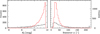 |
Fig. 7 Histograms of objects in the full sample: non-galaxies are in black and galaxies in red. Left: Extinction-corrected |
![Mathematical equation: $\[K_{\mathrm{s}}^{\mathrm{o}}\]$](/articles/aa/full_html/2025/12/aa57203-25/aa57203-25-eq62.png)
Statistics on some parameters for the sub-samples.
5.3 Extended sample
We also derived a sample by applying a diameter-dependent extinction correction as explained above (and, in more detail, in Paper I). Since this is an additional correction, our sample is not complete anymore and we have to add those objects that have ![Mathematical equation: $\[K_{\mathrm{s}}^{\mathrm{o}}>11^{\mathrm{m}}_\cdot 75\]$](/articles/aa/full_html/2025/12/aa57203-25/aa57203-25-eq63.png) but
but ![Mathematical equation: $\[K_{\mathrm{s}}^{\mathrm{o}, \mathrm{d}} \leq 11^{\mathrm{m}}_\cdot 75\]$](/articles/aa/full_html/2025/12/aa57203-25/aa57203-25-eq64.png) . The supplementary sample, labelled S+, comprises 1083 objects (see last entry in Table 5) and increases the galaxy sample by about 9%. The combined sample is called extended sample or Se.
. The supplementary sample, labelled S+, comprises 1083 objects (see last entry in Table 5) and increases the galaxy sample by about 9%. The combined sample is called extended sample or Se.
The galaxies in the supplementary sample are faint, with a lower limit of ![Mathematical equation: $\[K_{\mathrm{s}}^{\mathrm{o}, \mathrm{d}}=11^{\mathrm{m}}_\cdot00\]$](/articles/aa/full_html/2025/12/aa57203-25/aa57203-25-eq65.png) as shown in Fig. 9 in blue. For comparison, the full sample is shown in red. Note that we use the appropriately corrected Ks band magnitude for each sample. We also show the distribution with diameter, with a maximum diameter ad = 61″ for S+.
as shown in Fig. 9 in blue. For comparison, the full sample is shown in red. Note that we use the appropriately corrected Ks band magnitude for each sample. We also show the distribution with diameter, with a maximum diameter ad = 61″ for S+.
The histograms over Galactic latitude, stellar densities and extinction are shown in Figures 10 and 11. Here, we compare, on the one hand, the full sample S with the extended sample Se (in green and cyan, respectively), and, on the other hand, the two faint sub-samples S3 and S3e with corrected magnitudes in the range ![Mathematical equation: $\[11^{\mathrm{m}}_\cdot50-11^{\mathrm{m}}_\cdot75\]$](/articles/aa/full_html/2025/12/aa57203-25/aa57203-25-eq66.png) (in magenta and black, respectively). For interest, we have added the S+ sample in dotted grey line. The differences between the two faint samples seem small, but the distribution of the S+ galaxies with a marked peak around the Galactic plane shows the importance of this sample for the completion rate. This is more pronounced in Fig. 11, where the S+ distribution with extinction shows a clear increase, resulting in the S3e sample to show a more even distribution with extinction than S3. We estimate the completion in the Se sample is about
(in magenta and black, respectively). For interest, we have added the S+ sample in dotted grey line. The differences between the two faint samples seem small, but the distribution of the S+ galaxies with a marked peak around the Galactic plane shows the importance of this sample for the completion rate. This is more pronounced in Fig. 11, where the S+ distribution with extinction shows a clear increase, resulting in the S3e sample to show a more even distribution with extinction than S3. We estimate the completion in the Se sample is about ![Mathematical equation: $\[A_{\mathrm{K}}=1^{\mathrm{m}}_\cdot 3\]$](/articles/aa/full_html/2025/12/aa57203-25/aa57203-25-eq67.png) and possibly up to
and possibly up to ![Mathematical equation: $\[A_{\mathrm{K}}=1^{\mathrm{m}}_\cdot 5\]$](/articles/aa/full_html/2025/12/aa57203-25/aa57203-25-eq68.png) . The distribution with stellar densities appears unaffected.
. The distribution with stellar densities appears unaffected.
We added the statistics on the S+ sample to Table 6 though the total numbers of galaxies (587 and 18 in the ZOA and EBV samples, respectively) are small. Nonetheless, we can confirm that the trends with fainter samples hold for Disc class and velocities (with only 87 and 4 galaxies having a velocity measurement, respectively), while the extinction flags show a marked increase of almost a factor of two for the ZOA sample.
Colours are largely unaffected by the additional diameter-dependent extinction correction8, so we do not expect any qualitative differences in the mean or median. The change in sample size has only a negligible effect on the median values: we find 1.013 as compared to 1.011 for (J − Ks)o,c and 0.310 as compared to 0.309 for (H − Ks)o,c.
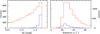 |
Fig. 9 Histograms of galaxies in the supplementary sample (S+, blue) as compared to the full sample (S, red). Left: extinction-corrected Ks band magnitude (with the diameter-dependent extinction correction applied for the S+ sample). Right: diameter in arcseconds (also corrected for the S+ sample). The red histograms are truncated. |
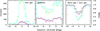 |
Fig. 10 Same as Fig. 6 but for the full sample S (green), Se (cyan), S3 (magenta), S3e (the faint sub-sample of the extended sample; black), and S+ (dotted grey). The left-hand panel shows non-galaxies instead of all sources and is truncated to emphasise the comparison of the faint samples. |
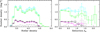 |
Fig. 11 Same as Fig. 8 but for the full sample S (green), Se (cyan), S3 (magenta), S3e (the faint sub-sample of the extended sample; black), and S+ (dotted grey). |
Statistics on 2MASX colours of various samples.
6 Galactic extinction
In Paper II we have used the colours of the bright sample to investigate how well the extinction map used represents the line-of-sight Galactic extinction. We can now do the same using the full sample. In the following we distinguish between the already applied correction factor of f = 0.86 and an additional factor fa, which should be multiplied with f to arrive at a final value fnew. From the slope of the extinction-corrected (J − Ks)o colour-extinction relation for the full sample, we have thus derived fa = 0.98 ± 0.01, which confirms that the correction factor derived in Paper II is still acceptable. For simplicity, the following discussion refers to fa only.
In contrast to Paper II, we excluded AGNs for this investigation (about 100 galaxies). While the effect on fa is minimal (0.982 versus 0.981 with AGNs included), the intercept becomes slightly redder by ![Mathematical equation: $\[0^{\mathrm{m}}_\cdot 003\]$](/articles/aa/full_html/2025/12/aa57203-25/aa57203-25-eq69.png) (which if of the order of the error on the intercept) when AGNs are included, emphasising their redder colour.
(which if of the order of the error on the intercept) when AGNs are included, emphasising their redder colour.
In Paper II, we mentioned the effect of applying an upper limit in AK on the slope of the fitted regression line. We reinvestigated this and find a stable plateau for the range ![Mathematical equation: $\[0^{\mathrm{m}}_\cdot 45< \lim(A_{K}) \leq 1^{\mathrm{m}}_\cdot 1\]$](/articles/aa/full_html/2025/12/aa57203-25/aa57203-25-eq70.png) for the new sample. Including galaxies at higher extinctions introduces a bias due to on-sky variations in extinction smaller than the resolution of the extinction maps. We thus use AK =
for the new sample. Including galaxies at higher extinctions introduces a bias due to on-sky variations in extinction smaller than the resolution of the extinction maps. We thus use AK = ![Mathematical equation: $\[1^{\mathrm{m}}_\cdot 1\]$](/articles/aa/full_html/2025/12/aa57203-25/aa57203-25-eq71.png) as the upper limit in our new investigation. Otherwise, we use the same selection criteria as in Paper II to ensure a photometrically clean sample.
as the upper limit in our new investigation. Otherwise, we use the same selection criteria as in Paper II to ensure a photometrically clean sample.
As discussed in Sect. 5.2, the fainter galaxies in our new sample are often more distant, which may require a k-correction. We have done two tests: firstly, we derived fa for the samples S1, S2 and S3 separately, see Table 8. We find that fa slightly decreases with the fainter samples, indicating that the k-correction indeed becomes relevant. Figure 12 shows the redshift distribution of the various samples, confirming the shift towards higher redshifts for the fainter samples. As a second test, we selected only galaxies that have redshift information and compared how fa changes when we apply the k-correction: The latter gives fa = 0.99 ± 0.01, as compared to fa = 0.98 ± 0.01 for the uncorrected ~4600 galaxies with redshift. The effect on the full sample is thus estimated to be negligible, though we should bear in mind a possible selection effect where predominantly brighter – and thus less distant – galaxies have been measured for redshift. Nonetheless, we expect the effect to be small, that is, less than the difference between the bright sample S1 and faint sample S3 (Δf < 0.02). In addition, we note that the intercept 1.00±0.00 when using the k-correction is the same as the median (J − Ks) colour for the high latitude bright sample (see Table 7).
With this information we were able to derive an improved ‘map’ of the f-values using bins in Galactic latitude and longitude. This helps in determining if there are intrinsic variations in the extinction properties across the Galactic plane. Since the binned samples are much smaller than the full sample, we kept the intercept fixed to the value derived for the full sample and fit only the slope for each bin (see Sect. 5 in Paper II for details on the derivation). Figure 13 gives Δf = fcell − fall, with the small, 60° × 5° cells in the top four rows, and larger, binned cells below (both in latitude, see, e.g. rows 5–7, and in longitude, see the bottom two panels). Contrary to Paper II, we used the neutral colour white for the range −0.01 < Δf < 0.01 (since 0.01 is the error on fa in the unbinned sample). We do not apply the k-correction so as to maximise the number of galaxies in the individual bins and to avoid possible selection effects by uneven selection of galaxies that have or have not redshift measurements. We do need to keep in mind, though, a possible selection effect through largescale structures that may lead to more distant galaxies in one bin and not in another.
The map compares very well with the one for the bright sample (Fig. B4 in Paper II), with the exception of a stronger deviation in the range 210° < l < 330°, which coincides with the direction of the dipole of the cosmic microwave background. However, no deviation is seen in the opposite direction. We need to keep in mind that overall the deviations shown in the map are mostly smaller than 3σ and thus not significant. Nonetheless, the negative Δf-values seen for those bins seem systematic and thus merit attention.
As a test, we applied the k-correction, keeping in mind the above mentioned caveats. The systematics in the range 210° < l < 270° have disappeared and lessened in the adjacent direction 270° < l < 330°, indicating that the deviation we see in Fig. 13 is likely due to selection effects through cosmic variance (note that both the Great Attractor as well as the Vela supercluster are found in this direction).
Object samples at different stages during extraction.
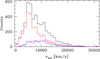 |
Fig. 12 Histogram of the redshift distribution of galaxies in the clean sample (black). The x-axis is truncated; there are six more galaxies between v = 32 000 km s−1 and 56 360 km s−1. Also shown are the histograms for the sub-samples S1 (red), S2 (blue) and S3 (magenta). |
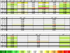 |
Fig. 13 Binned sky map with Δfa-values (fcell − fall) per cell. The colour scale is shown at the bottom. Red numbers may be overestimated, and colons indicate uncertain values. The 330°−210° cells are wrapped around the Galactic Centre. |
7 Summary
We have presented the full 2MZoA catalogue with an extinction corrected magnitude limit of ![Mathematical equation: $\[K_{\mathrm{s}}^{\mathrm{o}}=11^{\mathrm{m}}_\cdot 75\]$](/articles/aa/full_html/2025/12/aa57203-25/aa57203-25-eq72.png) , covering the ZoA at latitudes |b| < 10° (ZOA sample) and areas of high extinction (E(B − V) >
, covering the ZoA at latitudes |b| < 10° (ZOA sample) and areas of high extinction (E(B − V) > ![Mathematical equation: $\[0^{\mathrm{m}}_\cdot 950\]$](/articles/aa/full_html/2025/12/aa57203-25/aa57203-25-eq73.png) ; EBV sample) elsewhere. It thus serves as a complement to the 2MRS galaxy catalogue, resulting in the uniquely all-sky e2MRS survey. The catalogue comprises a total of 10 493 objects, of which 6899 are galaxies. Of the latter, 6757 are found in the ZOA sample, and 142 galaxies in the EBV sample. Compared to the catalogue of bright (
; EBV sample) elsewhere. It thus serves as a complement to the 2MRS galaxy catalogue, resulting in the uniquely all-sky e2MRS survey. The catalogue comprises a total of 10 493 objects, of which 6899 are galaxies. Of the latter, 6757 are found in the ZOA sample, and 142 galaxies in the EBV sample. Compared to the catalogue of bright (![Mathematical equation: $\[K_{\mathrm{s}}^{\mathrm{o}} \leq 11^{\mathrm{m}}_\cdot 25\]$](/articles/aa/full_html/2025/12/aa57203-25/aa57203-25-eq74.png) ) galaxies presented in Paper I, we have elected to use a different map of foreground extinction (the so-called GNILC extinction map by Planck Collaboration Int. XLVIII 2016), with a correction factor of f = 0.86 (see Paper II). We have also updated object classes (due to improved redshift and NIR information that have become available in the mean-time), added a flag to identify quasars and active galaxies, revisited the extinction flag settings, and added redshift information.
) galaxies presented in Paper I, we have elected to use a different map of foreground extinction (the so-called GNILC extinction map by Planck Collaboration Int. XLVIII 2016), with a correction factor of f = 0.86 (see Paper II). We have also updated object classes (due to improved redshift and NIR information that have become available in the mean-time), added a flag to identify quasars and active galaxies, revisited the extinction flag settings, and added redshift information.
We have discussed the properties of this new catalogue and have investigated possible differences to the bright sample (![Mathematical equation: $\[K_{\mathrm{s}}^{\mathrm{o}} \leq 11^{\mathrm{m}}_\cdot 25\]$](/articles/aa/full_html/2025/12/aa57203-25/aa57203-25-eq75.png) ) due to the increased number of smaller and more distant galaxies. We have found that the fainter sample is less contaminated by non-galaxian objects like Galactic Nebulae. However, the fainter sample is more affected by Galactic foreground extinction and is, in contrast to the bright sample, not complete anymore even at low extinction levels. Stellar densities also seem to have an increased effect on the completion levels. We also find less redshift information in the literature for the fainter galaxies which, often due to high foreground extinction, are more difficult to observe spectroscopically. Based on the colours of the faintest galaxies (
) due to the increased number of smaller and more distant galaxies. We have found that the fainter sample is less contaminated by non-galaxian objects like Galactic Nebulae. However, the fainter sample is more affected by Galactic foreground extinction and is, in contrast to the bright sample, not complete anymore even at low extinction levels. Stellar densities also seem to have an increased effect on the completion levels. We also find less redshift information in the literature for the fainter galaxies which, often due to high foreground extinction, are more difficult to observe spectroscopically. Based on the colours of the faintest galaxies (![Mathematical equation: $\[11^{\mathrm{m}}_\cdot 50<K_{\mathrm{s}}^{\mathrm{o}} \leq 11^{\mathrm{m}}_\cdot 75\]$](/articles/aa/full_html/2025/12/aa57203-25/aa57203-25-eq76.png) ), many of these are distant galaxies and would require a k-correction.
), many of these are distant galaxies and would require a k-correction.
We have also compiled a supplementary sample of galaxies that become brighter than the magnitude cut when we apply an additional extinction-corrected diameter correction (see Paper I for details), resulting in 1083 additional objects, of which 587 are galaxies. The additional galaxies are predominantly found at high extinctions, improving the completion levels of the combined (‘extended’) sample for extinctions up to ![Mathematical equation: $\[A_{\mathrm{K}}<1^{\mathrm{m}}_\cdot3\]$](/articles/aa/full_html/2025/12/aa57203-25/aa57203-25-eq77.png) and possibly beyond.
and possibly beyond.
Finally, according to the recipe presented in Paper II, we have compiled a binned sky map of the correction factor f to be applied to the Galactic foreground extinction. Though we have found larger deviations between cells than in Paper II, they are all within the 3σ errors, and the possible systematics found are likely due to cosmic variance. The full sample results in a correction factor of fnew = 0.84 ± 0.01, but due to the uncertainties in colours at the fainter end of our sample we continue to recommend the correction factor of f = 0.86 ± 0.01 as derived in Paper II.
The next steps in completing this project are as follows. (1) Improving the completion rate in the high stellar density area close to the Galactic Bulge could be achieved via by-eye searches and/or machine learning techniques (which might require additional by-eye verification, although the number of objects that needed visual inspection would be greatly reduced) of 2MASS images. Even more helpful would be searching the available deeper NIR images where the star crowding is alleviated through the higher spatial resolution of the images. Galaxy catalogues extracted from the VVV(X) surveys are already available (e.g. Alonso et al. 2025 and references therein). The drawback is that combining these catalogues with ours would lead to an inhomogeneously compiled 2MZoA catalogue, which would need careful calibration and adjustments.
(2) An improvement of galaxy photometry is important for the cosmic flow field analysis. A semi-automated script that automatically subtracts stars and extracts galaxy photometry combined with a thorough by-eye quality control (e.g. Said 2017) would also remove some of the uncertainties in the magnitude limit of the sample.
(3) For completing the redshift survey, we need to obtain the missing redshifts. These would also help to improve the accuracy of the galaxy photometry via a consistent application of the k-correction for all galaxies. Redshift completeness can be achieved using the new generation of radio telescopes, the SKA and SKA precursors, for H I observations, and large ground based telescopes like SALT and HET or space telescopes such as JWST for high quality IR of NIR spectroscopy.
Combined with the 2MRS, the here presented complementary catalogue forms the extended 2MRS survey, e2MRS, which comprises a nearly complete and homogeneous, magnitude-limited, all-sky galaxy catalogue. Apart from a small area (<4% of the whole sky) in the direction of the Galactic Bulge, where galaxy detection is severely restricted by high stellar densities, e2MRS can be considered as unbiased. As such it is invaluable for studies of large-scale structures, flow fields and extinction across the whole sky including the ZoA.
Data availability
Tables A.1, A.2, A.3 and A.4 are available at the CDS via https://cdsarc.cds.unistra.fr/viz-bin/cat/J/A+A/704/A252.
Acknowledgements
The authors thank Lucas Macri for access to the most updated 2MRS data set. This research has made use of data products from the Two Micron All Sky Survey, which is a joint project of the University of Massachusetts and the Infrared Processing and Analysis Center, funded by the National Aeronautics and Space Administration and the National Science Foundation. This research also has made use of the HyperLeda database, the SIMBAD database, operated at CDS, Strasbourg, France, the NASA/IPAC Extragalactic Database (NED), which is operated by the Jet Propulsion Laboratory, California Institute of Technology, under contract with the National Aeronautics and Space Administration and the Digitized Sky Surveys, which were produced at the Space Telescope Science Institute under U.S. Government grant NAG W-2166. This research has made use of the VizieR catalogue access tool, CDS, Strasbourg, France. The original description of the VizieR service was published in Ochsenbein et al. (2000). This research has made use of the Astrophysics Data System, funded by NASA under Cooperative Agreement 80NSSC25M7105.
References
- Acker, A., Stenholm, B., & Veron, P. 1991, A&AS, 87, 499 [Google Scholar]
- Alam, S., Albareti, F. D., Allende Prieto, C., et al. 2015, ApJS, 219, 12 [Google Scholar]
- Alonso, M. V., Baravalle, L. D., Nilo-Castellón, J. L., et al. 2025, A&A, 700, A33 [NASA ADS] [CrossRef] [EDP Sciences] [Google Scholar]
- Beuing, J., Bender, R., Mendes de Oliveira, C., Thomas, D., & Maraston, C. 2002, A&A, 395, 431 [NASA ADS] [CrossRef] [EDP Sciences] [Google Scholar]
- Bicay, M. D., & Giovanelli, R. 1986a, AJ, 91, 705 [Google Scholar]
- Bicay, M. D., & Giovanelli, R. 1986b, AJ, 91, 732 [Google Scholar]
- Bicay, M. D., & Giovanelli, R. 1987, AJ, 93, 1326 [Google Scholar]
- Bilicki, M., Jarrett, T. H., Peacock, J. A., Cluver, M. E., & Steward, L. 2014, ApJS, 210, 9 [Google Scholar]
- Bottinelli, L., Durand, N., Fouque, P., et al. 1992, A&AS, 93, 173 [NASA ADS] [Google Scholar]
- Bottinelli, L., Durand, N., Fouque, P., et al. 1993, A&AS, 102, 57 [NASA ADS] [Google Scholar]
- Bottinelli, L., Gouguenheim, L., Loulergue, M., et al. 1994, in Astronomical Society of the Pacific Conference Series, 67, Unveiling Large-Scale Structures Behind the Milky Way, eds. C. Balkowski & R. C. Kraan-Korteweg, 225 [Google Scholar]
- Braun, R., Thilker, D., & Walterbos, R. A. M. 2003, A&A, 406, 829 [NASA ADS] [CrossRef] [EDP Sciences] [Google Scholar]
- Burton, W. B., Verheijen, M. A. W., Kraan-Korteweg, R. C., & Henning, P. A. 1996, A&A, 309, 687 [Google Scholar]
- Chamaraux, P., Cayatte, V., Balkowski, C., & Fontanelli, P. 1990, A&A, 229, 340 [NASA ADS] [Google Scholar]
- Chamaraux, P., Kazes, I., Saito, M., Yamada, T., & Takata, T. 1995, A&A, 299, 347 [Google Scholar]
- Chamaraux, P., Masnou, J.-L., Kazés, I., et al. 1999, MNRAS, 307, 236 [Google Scholar]
- Collobert, M., Sarzi, M., Davies, R. L., Kuntschner, H., & Colless, M. 2006, MNRAS, 370, 1213 [Google Scholar]
- Corwin, Jr., H. G., & Emerson, D. 1982, MNRAS, 200, 621 [Google Scholar]
- Cote, S., Freeman, K. C., Carignan, C., & Quinn, P. J. 1997, AJ, 114, 1313 [CrossRef] [Google Scholar]
- Courtois, H. M., Tully, R. B., Fisher, J. R., et al. 2009, AJ, 138, 1938 [Google Scholar]
- Courtois, H. M., Tully, R. B., Makarov, D. I., et al. 2011, MNRAS, 414, 2005 [Google Scholar]
- Crawford, C. S., Edge, A. C., Fabian, A. C., et al. 1995, MNRAS, 274, 75 [NASA ADS] [CrossRef] [Google Scholar]
- Crook, A. C., Huchra, J. P., Martimbeau, N., et al. 2007, ApJ, 655, 790 [Google Scholar]
- Davies, R. L., Burstein, D., Dressler, A., et al. 1987, ApJS, 64, 581 [Google Scholar]
- Davies, R. D., Staveley-Smith, L., & Murray, J. D. 1989, MNRAS, 236, 171 [Google Scholar]
- Davoust, E., & Considere, S. 1995, A&AS, 110, 19 [NASA ADS] [Google Scholar]
- Daza-Perilla, I. V., Sgró, M. A., Baravalle, L. D., et al. 2023, MNRAS, 524, 678 [NASA ADS] [CrossRef] [Google Scholar]
- di Nella, H., Paturel, G., Walsh, A. J., et al. 1996, A&AS, 118, 311 [Google Scholar]
- di Nella, H., Couch, W. J., Parker, Q. A., & Paturel, G. 1997, MNRAS, 287, 472 [Google Scholar]
- Djorgovski, S., Thompson, D. J., de Carvalho, R. R., & Mould, J. R. 1990, AJ, 100, 599 [Google Scholar]
- Donley, J. L., Staveley-Smith, L., Kraan-Korteweg, R. C., et al. 2005, AJ, 129, 220 [NASA ADS] [CrossRef] [Google Scholar]
- Donley, J. L., Koribalski, B. S., Staveley-Smith, L., et al. 2006, MNRAS, 369, 1741 [Google Scholar]
- Dressler, A. 1991, ApJS, 75, 241 [Google Scholar]
- Dressler, A., Lynden-Bell, D., Burstein, D., et al. 1987, ApJ, 313, 42 [Google Scholar]
- Dupuy, A., Courtois, H. M., Guinet, D., Tully, R. B., & Kourkchi, E. 2021, A&A, 646, A113 [NASA ADS] [CrossRef] [EDP Sciences] [Google Scholar]
- Durret, F., Wakamatsu, K., Nagayama, T., Adami, C., & Biviano, A. 2015, A&A, 583, A124 [NASA ADS] [CrossRef] [EDP Sciences] [Google Scholar]
- Dutra, C. M., Ahumada, A. V., Clariá, J. J., Bica, E., & Barbuy, B. 2003, A&A, 408, 287 [NASA ADS] [CrossRef] [EDP Sciences] [Google Scholar]
- Dye, S., Lawrence, A., Read, M. A., et al. 2018, MNRAS, 473, 5113 [Google Scholar]
- Ebeling, H., Mullis, C. R., & Tully, R. B. 2002, ApJ, 580, 774 [Google Scholar]
- Eracleous, M., & Halpern, J. P. 2004, ApJS, 150, 181 [NASA ADS] [CrossRef] [Google Scholar]
- Fairall, A. P. 1983, MNRAS, 203, 47 [Google Scholar]
- Fairall, A. P. 1988a, MNRAS, 230, 69 [Google Scholar]
- Fairall, A. P. 1988b, MNRAS, 233, 691 [Google Scholar]
- Fairall, A. P., & Woudt, P. A. 2006, MNRAS, 366, 267 [Google Scholar]
- Fairall, A. P., Vettolani, G., & Chincarini, G. 1989, A&AS, 78, 269 [Google Scholar]
- Fairall, A. P., Woudt, P. A., & Kraan-Korteweg, R. C. 1998, A&AS, 127, 463 [NASA ADS] [CrossRef] [EDP Sciences] [Google Scholar]
- Falco, E. E., Kurtz, M. J., Geller, M. J., et al. 1999, PASP, 111, 438 [Google Scholar]
- Fisher, K. B., Huchra, J. P., Strauss, M. A., et al. 1995, ApJS, 100, 69 [Google Scholar]
- Fitzpatrick, E. L. 1999, PASP, 111, 63 [Google Scholar]
- Focardi, P., Marano, B., & Vettolani, G. 1984, A&A, 136, 178 [NASA ADS] [Google Scholar]
- Freeman, K. C., Karlsson, B., Lynga, G., et al. 1977, A&A, 55, 445 [NASA ADS] [Google Scholar]
- Freudling, W. 1995, A&AS, 112, 429 [NASA ADS] [Google Scholar]
- Fuerst, E., Reich, W., Kuehr, H., & Stickel, M. 1989, A&A, 223, 66 [Google Scholar]
- Giovanelli, R., & Haynes, M. P. 1981, AJ, 86, 340 [Google Scholar]
- Giovanelli, R., & Haynes, M. P. 1982, AJ, 87, 1355 [Google Scholar]
- Golovich, N., van Weeren, R. J., Dawson, W. A., Jee, M. J., & Wittman, D. 2017, ApJ, 838, 110 [NASA ADS] [CrossRef] [Google Scholar]
- Gordon, D., & Gottesman, S. T. 1981, AJ, 86, 161 [NASA ADS] [CrossRef] [Google Scholar]
- Hasegawa, T., Wakamatsu, K.-i., Malkan, M., et al. 2000, MNRAS, 316, 326 [Google Scholar]
- Hauschildt, M. 1987, A&A, 184, 43 [Google Scholar]
- Haynes, M. P., Giovanelli, R., Herter, T., et al. 1997, AJ, 113, 1197 [Google Scholar]
- Haynes, M. P., Giovanelli, R., Kent, B. R., et al. 2018, ApJ, 861, 49 [Google Scholar]
- Henning, P. A., Springob, C. M., Minchin, R. F., et al. 2010, AJ, 139, 2130 [Google Scholar]
- Hong, T., Staveley-Smith, L., Masters, K. L., et al. 2013, MNRAS, 432, 1178 [NASA ADS] [CrossRef] [Google Scholar]
- Huchra, J. P., Geller, M. J., Clemens, C. M., Tokarz, S. P., & Michel, A. 1992, Bull. Inform. Centre Donnees Stellaires, 41, 31 [Google Scholar]
- Huchra, J. P., Macri, L. M., Masters, K. L., et al. 2012, ApJS, 199, 26 [Google Scholar]
- Huchtmeier, W. K., Lercher, G., Seeberger, R., Saurer, W., & Weinberger, R. 1995, A&A, 293, L33 [Google Scholar]
- Huchtmeier, W. K., Karachentsev, I. D., Karachentseva, V. E., & Ehle, M. 2000, A&AS, 141, 469 [NASA ADS] [CrossRef] [EDP Sciences] [Google Scholar]
- Huchtmeier, W. K., Karachentsev, I. D., & Karachentseva, V. E. 2001, A&A, 377, 801 [NASA ADS] [CrossRef] [EDP Sciences] [Google Scholar]
- Huchtmeier, W. K., Karachentsev, I. D., & Karachentseva, V. E. 2003, A&A, 401, 483 [CrossRef] [EDP Sciences] [Google Scholar]
- Huchtmeier, W. K., Karachentsev, I. D., Karachentseva, V. E., Kudrya, Y. N., & Mitronova, S. N. 2005, A&A, 435, 459 [NASA ADS] [CrossRef] [EDP Sciences] [Google Scholar]
- Hudson, M. J., Smith, R. J., Lucey, J. R., & Branchini, E. 2004, MNRAS, 352, 61 [Google Scholar]
- Hunstead, R. W., Murdoch, H. S., & Shobbrook, R. R. 1978, MNRAS, 185, 149 [NASA ADS] [Google Scholar]
- Im, M., Lee, I., Cho, Y., et al. 2007, ApJ, 664, 64 [NASA ADS] [CrossRef] [Google Scholar]
- Iwata, I., & Chamaraux, P. 2011, A&A, 531, A87 [NASA ADS] [CrossRef] [EDP Sciences] [Google Scholar]
- Jarrett, T. H. 2004, PASA, 21, 396 [Google Scholar]
- Jarrett, T. H., Chester, T., Cutri, R., et al. 2000, AJ, 120, 298 [Google Scholar]
- Jarrett, T. H., Cohen, M., Masci, F., et al. 2011, ApJ, 735, 112 [Google Scholar]
- Jones, P. A., & McAdam, W. B. 1992, ApJS, 80, 137 [CrossRef] [Google Scholar]
- Jones, D. H., Saunders, W., Read, M., & Colless, M. 2005, PASA, 22, 277 [Google Scholar]
- Jones, D. H., Read, M. A., Saunders, W., et al. 2009, MNRAS, 399, 683 [Google Scholar]
- Kobulnicky, H. A., Dickey, J. M., Sargent, A. I., Hogg, D. E., & Conti, P. S. 1995, AJ, 110, 116 [NASA ADS] [CrossRef] [Google Scholar]
- Koss, M. J., Ricci, C., Trakhtenbrot, B., et al. 2022a, ApJS, 261, 2 [Google Scholar]
- Koss, M. J., Trakhtenbrot, B., Ricci, C., et al. 2022b, ApJS, 261, 6 [Google Scholar]
- Kourkchi, E., & Tully, R. B. 2017, ApJ, 843, 16 [NASA ADS] [CrossRef] [Google Scholar]
- Kraan-Korteweg, R. C., & Huchtmeier, W. K. 1992, A&A, 266, 150 [Google Scholar]
- Kraan-Korteweg, R. C., & Lahav, O. 2000, A&Ar, 10, 211 [Google Scholar]
- Kraan-Korteweg, R. C., Fairall, A. P., & Balkowski, C. 1995, A&A, 297, 617 [NASA ADS] [Google Scholar]
- Kraan-Korteweg, R. C., Woudt, P. A., Cayatte, V., et al. 1996, Nature, 379, 519 [NASA ADS] [CrossRef] [Google Scholar]
- Kraan-Korteweg, R. C., Henning, P. A., & Schröder, A. C. 2002, A&A, 391, 887 [NASA ADS] [CrossRef] [EDP Sciences] [Google Scholar]
- Kraan-Korteweg, R. C., Cluver, M. E., Bilicki, M., et al. 2017, MNRAS, 466, L29 [NASA ADS] [CrossRef] [Google Scholar]
- Kraan-Korteweg, R. C., van Driel, W., Schröder, A. C., Ramatsoku, M., & Henning, P. A. 2018, MNRAS, 481, 1262 [Google Scholar]
- Kregel, M., van der Kruit, P. C., & de Blok, W. J. G. 2004, MNRAS, 352, 768 [NASA ADS] [CrossRef] [Google Scholar]
- Lahav, O., Brosch, N., Goldberg, E., et al. 1998, MNRAS, 299, 24 [Google Scholar]
- Lang, R. H., Boyce, P. J., Kilborn, V. A., et al. 2003, MNRAS, 342, 738 [NASA ADS] [CrossRef] [Google Scholar]
- Lara, L., Márquez, I., Cotton, W. D., et al. 2001, A&A, 378, 826 [NASA ADS] [CrossRef] [EDP Sciences] [Google Scholar]
- Lavaux, G., & Hudson, M. J. 2011, MNRAS, 416, 2840 [Google Scholar]
- Lawrence, A., Rowan-Robinson, M., Ellis, R. S., et al. 1999, MNRAS, 308, 897 [Google Scholar]
- Ledlow, M. J., Owen, F. N., & Miller, N. A. 2005, AJ, 130, 47 [Google Scholar]
- Lewis, B. M., Helou, G., & Salpeter, E. E. 1985, ApJS, 59, 161 [Google Scholar]
- Liu, X.-W., Zhao, G., & Hou, J.-L. 2015, Res. Astron. Astrophys., 15, 1089 [CrossRef] [Google Scholar]
- Lu, N. Y., & Freudling, W. 1995, ApJ, 449, 527 [Google Scholar]
- Lu, N. Y., Dow, M. W., Houck, J. R., Salpeter, E. E., & Lewis, B. M. 1990, ApJ, 357, 388 [Google Scholar]
- Lucas, P. W., Hoare, M. G., Longmore, A., et al. 2008, MNRAS, 391, 136 [Google Scholar]
- Macri, L. M., Kraan-Korteweg, R. C., Lambert, T., et al. 2019, ApJS, 245, 6 [Google Scholar]
- Martin, J. M., Bottinelli, L., Dennefeld, M., et al. 1990, A&A, 235, 41 [Google Scholar]
- Martin, J. M., Bottinelli, L., Dennefeld, M., & Gouguenheim, L. 1991, A&A, 245, 393 [NASA ADS] [Google Scholar]
- Marzke, R. O., Huchra, J. P., & Geller, M. J. 1996, AJ, 112, 1803 [Google Scholar]
- Masetti, N., Mason, E., Morelli, L., et al. 2008, A&A, 482, 113 [NASA ADS] [CrossRef] [EDP Sciences] [Google Scholar]
- Masetti, N., Parisi, P., Palazzi, E., et al. 2010, A&A, 519, A96 [NASA ADS] [CrossRef] [EDP Sciences] [Google Scholar]
- Masters, K. L., Crook, A., Hong, T., et al. 2014, MNRAS, 443, 1044 [NASA ADS] [CrossRef] [Google Scholar]
- Mathewson, D. S., & Ford, V. L. 1996, ApJS, 107, 97 [Google Scholar]
- McIntyre, T. P., Henning, P. A., Minchin, R. F., Momjian, E., & Butcher, Z. 2015, AJ, 150, 28 [NASA ADS] [CrossRef] [Google Scholar]
- Meyer, M. J., Zwaan, M. A., Webster, R. L., et al. 2004, MNRAS, 350, 1195 [Google Scholar]
- Minniti, D., Lucas, P. W., Emerson, J. P., et al. 2010, New Astron., 15, 433 [Google Scholar]
- Mitronova, S. N., Huchtmeier, W. K., Karachentsev, I. D., Karachentseva, V. E., & Kudrya, Y. N. 2005, Astron. Lett., 31, 501 [Google Scholar]
- Monnier Ragaigne, D., van Driel, W., O’Neil, K., et al. 2003, A&A, 408, 67 [NASA ADS] [CrossRef] [EDP Sciences] [Google Scholar]
- Morganti, R., Emonts, B., & Oosterloo, T. 2009, A&A, 496, L9 [NASA ADS] [CrossRef] [EDP Sciences] [Google Scholar]
- Motch, C., Guillout, P., Haberl, F., et al. 1998, A&AS, 132, 341 [NASA ADS] [CrossRef] [EDP Sciences] [Google Scholar]
- Nakanishi, K., Takata, T., Yamada, T., et al. 1997, ApJS, 112, 245 [Google Scholar]
- Nilsson, K., Pursimo, T., Heidt, J., et al. 2003, A&A, 400, 95 [NASA ADS] [CrossRef] [EDP Sciences] [Google Scholar]
- Ochsenbein, F., Bauer, P., & Marcout, J. 2000, A&AS, 143, 23 [NASA ADS] [CrossRef] [EDP Sciences] [Google Scholar]
- Ogando, R. L. C., Maia, M. A. G., Pellegrini, P. S., & da Costa, L. N. 2008, AJ, 135, 2424 [NASA ADS] [CrossRef] [Google Scholar]
- Owen, F. N., Ledlow, M. J., Morrison, G. E., & Hill, J. M. 1997, ApJ, 488, L15 [Google Scholar]
- Pantoja, C. A., Giovanardi, C., Altschuler, D. R., & Giovanelli, R. 1994, AJ, 108, 921 [Google Scholar]
- Pantoja, C. A., Altschuler, D. R., Giovanardi, C., & Giovanelli, R. 1997, AJ, 113, 905 [Google Scholar]
- Paturel, G., Theureau, G., Bottinelli, L., et al. 2003, A&A, 412, 57 [NASA ADS] [CrossRef] [EDP Sciences] [Google Scholar]
- Pesce, D. W., Braatz, J. A., Condon, J. J., & Greene, J. E. 2018, ApJ, 863, 149 [CrossRef] [Google Scholar]
- Planck Collaboration Int. XLVIII. 2016, A&A, 596, A109 [NASA ADS] [CrossRef] [EDP Sciences] [Google Scholar]
- Proust, D., Mazure, A., Vanderriest, C., Sodre, Jr., L., & Capelato, H. V. 1995, A&AS, 114, 565 [Google Scholar]
- Radburn-Smith, D. J., Lucey, J. R., Woudt, P. A., Kraan-Korteweg, R. C., & Watson, F. G. 2006, MNRAS, 369, 1131 [NASA ADS] [CrossRef] [Google Scholar]
- Ramatsoku, M., Verheijen, M. A. W., Kraan-Korteweg, R. C., et al. 2016, MNRAS, 460, 923 [NASA ADS] [CrossRef] [Google Scholar]
- Riad, I. F., Kraan-Korteweg, R. C., & Woudt, P. A. 2010, MNRAS, 401, 924 [NASA ADS] [CrossRef] [Google Scholar]
- Roman, A. T., Takeuchi, T. T., Nakanishi, K., & Saito, M. 1998, PASJ, 50, 47 [Google Scholar]
- Rosenberg, J. L., & Schneider, S. E. 2000, ApJS, 130, 177 [NASA ADS] [CrossRef] [Google Scholar]
- Sadler, E. M. 1984, AJ, 89, 23 [Google Scholar]
- Said, K. 2017, Peculiar flow fields in the Zone of Avoidance from the nearinfrared Tully-Fisher relation, PhD Thesis, University of Cape Town [Google Scholar]
- Said, K., Kraan-Korteweg, R. C., Staveley-Smith, L., et al. 2016, MNRAS, 457, 2366 [NASA ADS] [CrossRef] [Google Scholar]
- Saito, R. K., Hempel, M., Alonso-García, J., et al. 2024, A&A, 689, A148 [NASA ADS] [CrossRef] [EDP Sciences] [Google Scholar]
- Sanchez-Barrantes, M., Henning, P. A., McIntyre, T., et al. 2019, AJ, 158, 234 [NASA ADS] [CrossRef] [Google Scholar]
- Sandage, A. 1976, PASP, 88, 367 [Google Scholar]
- Sanders, D. B., Egami, E., Lipari, S., Mirabel, I. F., & Soifer, B. T. 1995, AJ, 110, 1993 [Google Scholar]
- Sargent, W. L. W. 1973, ApJ, 182, L13 [Google Scholar]
- Saunders, W., Sutherland, W. J., Maddox, S. J., et al. 2000, MNRAS, 317, 55 [Google Scholar]
- Schlafly, E. F., Green, G. M., Lang, D., et al. 2018, ApJS, 234, 39 [Google Scholar]
- Schlegel, D. J., Finkbeiner, D. P., & Davis, M. 1998, ApJ, 500, 525 [Google Scholar]
- Schneider, S. E., Thuan, T. X., Mangum, J. G., & Miller, J. 1992, ApJS, 81, 5 [NASA ADS] [CrossRef] [Google Scholar]
- Schröder, A. C., Kraan-Korteweg, R. C., & Henning, P. A. 2009, A&A, 505, 1049 [NASA ADS] [CrossRef] [EDP Sciences] [Google Scholar]
- Schröder, A. C., Flöer, L., Winkel, B., & Kerp, J. 2019, MNRAS, 489, 2907 [Google Scholar]
- Schröder, A. C., van Driel, W., & Kraan-Korteweg, R. C. 2021, MNRAS, 503, 5351 [CrossRef] [Google Scholar]
- Schröder, A. C., van Driel, W., Kraan-Korteweg, R. C., & Belleval, C. 2025, A&A, 695, A79 [NASA ADS] [CrossRef] [EDP Sciences] [Google Scholar]
- Seeberger, R., & Saurer, W. 1998, A&AS, 127, 101 [NASA ADS] [CrossRef] [EDP Sciences] [Google Scholar]
- Seeberger, R., Huchtmeier, W. K., & Weinberger, R. 1994, A&A, 286, 17 [Google Scholar]
- Sekiguchi, K., & Wolstencroft, R. D. 1992, MNRAS, 255, 581 [Google Scholar]
- Skrutskie, M. F., Cutri, R. M., Stiening, R., et al. 2006, AJ, 131, 1163 [NASA ADS] [CrossRef] [Google Scholar]
- Spinrad, H. 1975, ApJ, 199, L1 [Google Scholar]
- Springob, C. M., Haynes, M. P., Giovanelli, R., & Kent, B. R. 2005, ApJS, 160, 149 [NASA ADS] [CrossRef] [Google Scholar]
- Springob, C. M., Hong, T., Staveley-Smith, L., et al. 2016, MNRAS, 456, 1886 [CrossRef] [Google Scholar]
- Staveley-Smith, L., Kraan-Korteweg, R. C., Schröder, A. C., et al. 2016, AJ, 151, 52 [Google Scholar]
- Strauss, M. A., Huchra, J. P., Davis, M., et al. 1992, ApJS, 83, 29 [Google Scholar]
- Sulentic, J. W., & Arp, H. 1983, AJ, 88, 489 [Google Scholar]
- Takata, T., Yamada, T., Saito, M., Chamaraux, P., & Kazes, I. 1994, A&AS, 104, 529 [Google Scholar]
- Theureau, G., Bottinelli, L., Coudreau-Durand, N., et al. 1998, A&AS, 130, 333 [NASA ADS] [CrossRef] [EDP Sciences] [Google Scholar]
- Theureau, G., Coudreau, N., Hallet, N., et al. 2005, A&A, 430, 373 [NASA ADS] [CrossRef] [EDP Sciences] [Google Scholar]
- Theureau, G., Hanski, M. O., Coudreau, N., Hallet, N., & Martin, J. M. 2007, A&A, 465, 71 [NASA ADS] [CrossRef] [EDP Sciences] [Google Scholar]
- Theureau, G., Coudreau, N., Hallet, N., Hanski, M. O., & Poulain, M. 2017, A&A, 599, A104 [NASA ADS] [CrossRef] [EDP Sciences] [Google Scholar]
- Tifft, W. G., & Cocke, W. J. 1988, ApJS, 67, 1 [Google Scholar]
- Tully, R. B. et al. 2008, ApJ, 676, 184 [Google Scholar]
- Tully, R. B., Pomarède, D., Graziani, R., et al. 2019, ApJ, 880, 24 [Google Scholar]
- van den Bosch, R. C. E., Gebhardt, K., Gültekin, K., Yıldırım, A., & Walsh, J. L. 2015, ApJS, 218, 10 [Google Scholar]
- Visvanathan, N., & van den Bergh, S. 1992, AJ, 103, 1057 [Google Scholar]
- Visvanathan, N., & Yamada, T. 1996, ApJS, 107, 521 [Google Scholar]
- Wegner, G., Bernardi, M., Willmer, C. N. A., et al. 2003, AJ, 126, 2268 [NASA ADS] [CrossRef] [Google Scholar]
- West, R. M., & Tarenghi, M. 1989, A&A, 223, 61 [NASA ADS] [Google Scholar]
- West, R. M., Surdej, J., Schuster, H. E., et al. 1981, A&AS, 46, 57 [Google Scholar]
- Wong, O. I., Ryan-Weber, E. V., Garcia-Appadoo, D. A., et al. 2006, MNRAS, 371, 1855 [Google Scholar]
- Woudt, P. A., Kraan-Korteweg, R. C., & Fairall, A. P. 1999, A&A, 352, 39 [NASA ADS] [Google Scholar]
- Woudt, P. A., Kraan-Korteweg, R. C., Cayatte, V., Balkowski, C., & Felenbok, P. 2004, A&A, 415, 9 [NASA ADS] [CrossRef] [EDP Sciences] [Google Scholar]
- Woudt, P. A., Kraan-Korteweg, R. C., Lucey, J., Fairall, A. P., & Moore, S. A. W. 2008, MNRAS, 383, 445 [Google Scholar]
- Wouterloot, J. G. A., & Brand, J. 1989, A&AS, 80, 149 [NASA ADS] [Google Scholar]
- Yamada, T., & Saito, M. 1993, PASJ, 45, 25 [Google Scholar]
- Yamada, T., Tomita, A., Saito, M., Chamaraux, P., & Kazes, I. 1994, MNRAS, 270, 93 [Google Scholar]
- Zirbel, E. L., & Baum, S. A. 1995, ApJ, 448, 521 [NASA ADS] [CrossRef] [Google Scholar]
- Zurita Heras, J. A., Chaty, S., & Tomsick, J. A. 2009, A&A, 502, 787 [NASA ADS] [CrossRef] [EDP Sciences] [Google Scholar]
See the 2MASS All-Sky Extended Source Catalog (XSC) as found online at https://irsa.ipac.caltech.edu/cgi-bin/Gator/nph-scan?mission=irsa&submit=Select&projshort=2MASS
e.g. UHS (UKIRT Hemisphere Survey, Dye et al. 2018) and VVVX (Saito et al. 2024) survey images have become available in the mean-time.
A third section comprises 12 additional galaxies neither included in the full nor in the supplementary sample but which have ![Mathematical equation: $\[K_{\mathrm{s}}^{\mathrm{o}} \leq 11^{\mathrm{m}}_\cdot 75\]$](/articles/aa/full_html/2025/12/aa57203-25/aa57203-25-eq80.png) if no correction factor is applied to the extinction; we only list these for the comparison of samples, they are not used elsewhere.
if no correction factor is applied to the extinction; we only list these for the comparison of samples, they are not used elsewhere.
for a detailed description see http://tdc-www.harvard.edu/2mrs/2mrs_readme.html
Though only objects flagged as galaxies (cf. Col. 7a) have velocity entries listed in the table, there are a few uncertain galaxies with questionable velocity measurements.
Some of the redshift measurements we use in our catalogue are work in progress and were obtained by members of our group and collaborators, see Schröder et al. (2021) for details.
The majority of which can be found in the 2MASS Photometric Redshift catalogue by Bilicki et al. (2014).
Colours are derived using a fixed aperture across all bands, and in the outer parts of a galaxy the colour changes only little with a further increase of the diameter.
Appendix A Tables
The four tables A.1 – A.4 are available electronically at the CDS. For clarity, we list in this section some example lines for each table.
Table A.1 presents the full catalogue. The columns are described in Sect. 3.
For the radial velocity information in Table A.1, we searched the literature for our objects. We were mainly interested in original measurements and do not list all available compilations. We searched online databases (NED, Simbad, Leda) as well as catalogues available at the CDS. Though we concentrated on objects classified as galaxies, we also searched systematically for object class 5 (unknown) and 6 (lower likelihood for being a galaxy) to be comprehensive.
The compilation of the velocities is given in Table A.2 for optical velocities, and in Table A.3 for H I measurements. The tables give one line per velocity and reference per object. They are ordered by (a) error (or quality) for original measurements, (b) re-reductions (unless superseding the original publication), (c) by publication year for referenced values (indicated by ‘c’; in Col. 2), and (d) averaged values or non-detection entries. Non-accepted values (for example detection of another galaxy nearby or wrong measurements) are marked in the flag column.
The columns in the two tables are as follows:
Col. 1: ID: 2MASX catalogue identification number (based on J2000.0 coordinates).
Cols. 2 − 5: Flags repeated from Cols 9, 4, 5 and 6 from Table A.1.
Cols. 6: Velocity measurement flags refering to the quoted publication. They are similar to the flags in Col. 10 of Table A.1 with the addition of ‘c’ for compilation, ‘a’ for compilation that gives averaged values, ‘r’ for re-reduced, and ‘n’ for non detections.
Cols. 7 − 9: Redshift value and error in kilometre per second and the bibcode of the reference (see Table A.4 for details).
Cols. 10: Comments. An arrow indicates a quoted reference (usually also listed by us in this table), single quotes refer to comments made in the publication. Where possible we give telescope or instrument information (see also Table A.4 for generic information regarding the publication).
Table A.4 lists the references used in Tables A.2 and A.3 with: (1) Bibcode; (2) Name of first author; (3) Source of data (either the wavelength regime or literature); (4) Observational and velocity information where relevant (e.g. telescope used, precision of the velocity); (5) Comments.
2MZoA sample Part I (example lines).
2MZoA sample Part II (example lines).
Optical velocity information (example lines).
H I velocity information (example lines).
References for the redshifts (examples).
Appendix B Sky maps
The on-sky distribution of both the ZOA and the EBV samples is shown in Fig. B.1, with galaxies shown in grey and non-galaxies in yellow. Magenta dots show galaxies from the extended sample (that is, with a diameter-dependent extinction correction applied). There are only a few areas at higher latitudes (b ≥ 10°) that have extinctions high enough to be in the EBV sample.
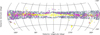 |
Fig. B.1 Aitoff projection in Galactic coordinates of the ZOA and EBV samples. Grey dots are galaxies, yellow dots non-galaxies, and green dots objects of unknown nature. Magenta dots indicate galaxies that are added through the diameter-depended extinction correction. |
All Tables
All Figures
|
Fig. 1 2MASS extinction-corrected colour–colour plot, (H − Ks)o versus (J − Ks)o. A reddening vector, representing the mean of the sample shown, is indicated by a red arrow in the bottom right corner. The reddening path for objects within the intrinsic colour range of galaxies is indicated with two parallel dashed lines. |
| In the text | |
|
Fig. 2 WISE extinction-corrected colour–colour plot, (W1 − W2)o versus (W2 − W3)o for the full sample. A reddening vector, representing the mean of the sample shown, is indicated by a red arrow in the top right corner. Open circles mark active galaxies as labelled. |
| In the text | |
|
Fig. 3 Histograms of objects in the ZOA sample as a function of Galactic latitude for all objects (blue) and for galaxies only (red). The black line represents the average 2MASX galaxy count outside the ZoA. Panel a: for all Galactic longitudes; panel b for the semi-circle towards the anti-centre region; panel c for the semi-circle towards the bulge. |
| In the text | |
|
Fig. 4 Histograms of the number density of all ZOA sample objects (blue) and galaxies only (red) as a function of stellar density (top panel) and Galactic extinction AK (bottom panel; only regions with log N*/deg2 ≤ 4.5 were used). The error bars indicate Poissonian errors per bin. The dotted black lines represent the average 2MASX bright galaxy number density outside of the ZoA. |
| In the text | |
|
Fig. 5 Normalised histograms of 2MASX colours (J − Ks)o (left) and (H − Ks)o (right). Green histograms are the full sample and the magenta histograms show colours corrected for stellar densities. the yellow-filled histograms represent the average high Galactic latitude sample. |
| In the text | |
|
Fig. 6 Histograms of objects in the ZOA samples with Galactic latitude: all objects (left), galaxies (middle), and the fraction of galaxies (right). S1 is shown in red, S2 in blue, and S3 in magenta. |
| In the text | |
|
Fig. 7 Histograms of objects in the full sample: non-galaxies are in black and galaxies in red. Left: Extinction-corrected |
| In the text | |
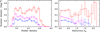 |
Fig. 8 Same as Fig. 4 but or the galaxies in the sub-samples S1 (red), S2 (blue), and S3 (magenta). |
| In the text | |
|
Fig. 9 Histograms of galaxies in the supplementary sample (S+, blue) as compared to the full sample (S, red). Left: extinction-corrected Ks band magnitude (with the diameter-dependent extinction correction applied for the S+ sample). Right: diameter in arcseconds (also corrected for the S+ sample). The red histograms are truncated. |
| In the text | |
|
Fig. 10 Same as Fig. 6 but for the full sample S (green), Se (cyan), S3 (magenta), S3e (the faint sub-sample of the extended sample; black), and S+ (dotted grey). The left-hand panel shows non-galaxies instead of all sources and is truncated to emphasise the comparison of the faint samples. |
| In the text | |
|
Fig. 11 Same as Fig. 8 but for the full sample S (green), Se (cyan), S3 (magenta), S3e (the faint sub-sample of the extended sample; black), and S+ (dotted grey). |
| In the text | |
|
Fig. 12 Histogram of the redshift distribution of galaxies in the clean sample (black). The x-axis is truncated; there are six more galaxies between v = 32 000 km s−1 and 56 360 km s−1. Also shown are the histograms for the sub-samples S1 (red), S2 (blue) and S3 (magenta). |
| In the text | |
|
Fig. 13 Binned sky map with Δfa-values (fcell − fall) per cell. The colour scale is shown at the bottom. Red numbers may be overestimated, and colons indicate uncertain values. The 330°−210° cells are wrapped around the Galactic Centre. |
| In the text | |
|
Fig. B.1 Aitoff projection in Galactic coordinates of the ZOA and EBV samples. Grey dots are galaxies, yellow dots non-galaxies, and green dots objects of unknown nature. Magenta dots indicate galaxies that are added through the diameter-depended extinction correction. |
| In the text | |
Current usage metrics show cumulative count of Article Views (full-text article views including HTML views, PDF and ePub downloads, according to the available data) and Abstracts Views on Vision4Press platform.
Data correspond to usage on the plateform after 2015. The current usage metrics is available 48-96 hours after online publication and is updated daily on week days.
Initial download of the metrics may take a while.