| Issue |
A&A
Volume 704, December 2025
|
|
|---|---|---|
| Article Number | A303 | |
| Number of page(s) | 21 | |
| Section | Extragalactic astronomy | |
| DOI | https://doi.org/10.1051/0004-6361/202557218 | |
| Published online | 17 December 2025 | |
Towards precision cosmology with improved PNLF distances using VLT-MUSE
III. Impact of stellar populations in early-type galaxies
1
Leibniz-Institut für Astrophysik Potsdam (AIP), An der Sternwarte 16, 14482 Potsdam, Germany
2
Institut für Physik und Astronomie, Universität Potsdam, Karl-Liebknecht-Str. 24/25, 14476 Potsdam, Germany
3
Universitäts-Sternwarte, Fakultät für Physik, Ludwig-Maximilians Universität München, Scheinerstr. 1, 81679 München, Germany
4
Deutsches Zentrum für Astrophysik (DZA), Postplatz 1, 02826 Görlitz, Germany
5
Department of Astronomy & Astrophysics, The Pennsylvania State University, University Park, PA 16802, USA
6
Institute for Gravitation and the Cosmos, The Pennsylvania State University, University Park, PA 16802, USA
7
NSF’s NOIRLab, 950 N. Cherry Ave., Tucson, AZ 85719, USA
8
European Southern Observatory, Karl-Schwarzschild-Straße 2, 85748 Garching, Germany
★ Corresponding author: This email address is being protected from spambots. You need JavaScript enabled to view it.
Received:
12
September
2025
Accepted:
27
October
2025
Abstract
Aims. Distance measurements using the planetary nebula luminosity function (PNLF) rely on the bright-end cutoff magnitude (M*), which is defined by a number of the [O III]λ5007-brightest planetary nebulae (PNe). In early-type galaxies (ETGs), the formation of these PNe is enigmatic; the population is typically too old to form the expected M* PNe from single star evolution. We aim to provide a viable solution to this problem.
Methods. We selected five ETGs with known MUSE-PNLF distances. The MUSE instrument allows us to calculate the PNLF and consistently investigate the underlying stellar populations. Using stellar population synthesis, we derived the population age, star formation history, metallicity, and alpha abundance. We compared these parameters to the PNLF variables: the absolute magnitude of the bright cutoff (M*) and luminosity-specific PN number at the top 0.5 mag of the PNLF (α0.5). We also compare our results with PNe In Cosmological Simulations (PICS) model applied to Magneticum Pathfinder analogue galaxies.
Results. The average mass-weighted ages and metallicities of the stellar populations in our datasets are typically old (9 < Age < 13.5 Gyr) and rather metal rich (−0.4 < [M/H] < +0.2). We find the value of M* to be independent of age and metallicity in these ages and metallicity intervals. We observed a positive correlation between α0.5 values and the mass fraction of stellar population ages of 2–10 Gyr, implying that most of the PNe originate from stars with intermediate ages. Similar trends are also found in the PICS analogue galaxies.
Conclusions. We show that when ∼2% of the stellar mass present is younger than 10 Gyr, it is sufficient to form the M* PNe in ETGs. We also present observing requirements for an ideal PNLF distance determination in ETGs.
Key words: stars: AGB and post-AGB / planetary nebulae: general / galaxies: distances and redshifts / galaxies: elliptical and lenticular / cD / galaxies: stellar content / distance scale
© The Authors 2025
 Open Access article, published by EDP Sciences, under the terms of the Creative Commons Attribution License (https://creativecommons.org/licenses/by/4.0), which permits unrestricted use, distribution, and reproduction in any medium, provided the original work is properly cited.
This article is published in open access under the Subscribe to Open model. This email address is being protected from spambots. You need JavaScript enabled to view it. to support open access publication.
1. Introduction
The planetary nebula luminosity function (PNLF) was proposed as a standard candle for extragalactic distance determinations more than 35 years ago (Jacoby 1989; Ciardullo et al. 1989). It relies on the empirical fact that narrow-band photometry in the emission line of [O III]λ5007, of a sufficiently large sample of planetary nebulae (PNe) in any galaxy shows a luminosity function with a well defined knee and bright-end cutoff magnitude (M*) that can serve as a standard candle. As explained in a review by Ciardullo (2022), in the first two decades of its use, the technique produced almost one hundred precise distance determinations out to 20 Mpc. However, interest in the method declined in the following years. In the early 2010s, direct calibration of supernova type Ia parent galaxies using Cepheids yielded ∼3% precision for the Hubble constant, H0 (Riess et al. 2011). This superseded the need for intermediate candles, such as the PNLF. Subsequently, Cepheid measurements in recent years pushed the H0 precision down to ∼1% (Riess et al. 2022), which was crucial to the emergence of the Hubble Tension (Di Valentino et al. 2021).
With the advent of MUSE (Multi Unit Spectral Explorer; Bacon et al. 2010) at the ESO Very Large Telescope (VLT), a more effective and versatile tool for narrow-band imaging became available. MUSE is an integral field spectrograph with a 1 arcmin2 field of view, excellent image quality, relatively high spectral resolution (R ∼ 2000), and high efficiency. The instrument offers many advantages over traditional narrow-band surveys for the detection of [O III]λ5007 point sources, including a much narrower effective bandpass and spectral information which immediately helps with the rejection of interlopers, such as H II regions, supernova remnants, and other bright emission-line sources (Herrmann et al. 2008; Herrmann & Ciardullo 2009; Kreckel et al. 2017; Aniyan et al. 2018).
Several authors (e.g. Spriggs et al. 2021; Scheuermann et al. 2022; Congiu et al. 2023; Soemitro et al. 2023; Congiu et al. 2025) have found the instrument to exceed the sensitivity and distance range accessible by classical narrow-band imaging. Roth et al. (2018) showed that by placing simulated point sources inside real MUSE data cubes, [O III]λ5007 photometry can be accomplished to magnitudes as faint as m5007 = 29. More importantly, Roth et al. (2021) (hereafter Paper I) discovered that the galaxy background continuum light, which must be subtracted during PN aperture photometry, can be estimated with great precision using the full spectrum information present in the data cube. Unlike the classical on-band–off-band measurements for the narrow-band filter technique, this enables the application of a self-calibrating background subtraction technique, called the differential emission line filter (DELF). In addition to the benefits of MUSE mentioned above, DELF provides an additional factor of two improvement over other detection techniques, as demonstrated with three benchmark galaxies (Paper I).
Encouraged by this finding and using the DELF technique, Jacoby et al. (2024, hereafter Paper II) analysed MUSE data cubes for 20 galaxies that were retrieved from the ESO archive, and determined their respective PNLFs. Although some of the data were taken in less-than-ideal observing conditions and despite the calibration issues associated with data taken for other purposes, this proof-of-principle study demonstrated that PNLF measurements with MUSE can yield 5% precision distances to individual galaxies. It also shows that the PNLF method can be pushed to distances as far as ∼40 Mpc with ground-based telescopes. This is comparable to the distance range of the best space-based observations of Cepheids (Riess et al. 2022) and the tip of the red giant branch (TRGB, Anand et al. 2024a), and well within the range of surface brightness fluctuations (SBF, Blakeslee et al. 2021) distances. Based on the studies presented in Papers I and II, and considering optimized observing strategies with MUSE, a renaissance of the PNLF is now possible.
Unlike Cepheid and TRGB distances that rely on well-established stellar physics (Bono et al. 2024; Beaton et al. 2018, and references therein), there are still uncertainties regarding the theoretical basis of the PNLF. The main aspect to understand is whether M* has some small dependence on a stellar population that has not been measured. While the effect of metallicity on PNLF distances is well understood (Dopita et al. 1992; Ciardullo et al. 2002; Valenzuela et al. 2025), its insensitivity to age is more problematic. This issue is critical, especially in old systems such as elliptical or lenticular galaxies.
According to most initial-final mass (IFMR) relations (e.g. Cummings et al. 2018; Cunningham et al. 2024), the observed PNLF cutoff implies a population of progenitor stars that are ∼3 Gyr or younger (Gesicki et al. 2018; Ciardullo 2022). Such stars are exceedingly rare in Population II systems and cannot account for the number of observed bright PNe, even though early-type galaxies (ETGs) harbour at least 1–2% of the stellar mass of populations younger than 1 Gyr (Yi et al. 2005). To overcome this, Ciardullo et al. (2005) attempted to explain this phenomenon through binary star evolution, and more recently, Valenzuela et al. (2025) argued that shifts in the IFMR with helium and metal abundance can achieve the canonical M* for populations as old as 10 Gyr. Additionally, Jacoby & Ciardullo (2025) suggested that a small amount of scatter in the IFMR, consistent with that used to explain the horizontal branch morphologies of old star clusters, could produce and maintain the cutoff PNe, even in the oldest systems. If true, this predicts a trend where the production rate of [O III]λ5007-bright PNe, and therefore the luminosity specific number of such objects (the α-parameter) declines with increasing population age (Ciardullo et al. 2005; Buzzoni et al. 2006). Higher α-parameter values have been reported in the outer haloes of three old elliptical galaxies (M87, M49, and M105), and linked to bluer, lower metallicity environments (Longobardi et al. 2015; Hartke et al. 2017, 2020). These studies examine how the PNLF is affected by stellar population changes, traced through colour gradients and colour–magnitude diagrams of resolved stellar populations.
In this third paper in the MUSE-PNLF series, we shed light on the physics behind the PNLF’s bright-end cutoff in ETGs. To do this, we used five ETGs with publicly available MUSE data from the ESO Archive (Romaniello 2022). For each galaxy, we used the MUSE data to measure the PNLF’s cutoff magnitude M* and normalization parameter α (the luminosity specific PN number) as a function of radius, and correlated these parameter values with the galaxies’ stellar population ages and metallicities, as derived from the population synthesis analyses of the galaxies’ MUSE spectra (Ennis et al. 2023). While the relation between the underlying stellar population and the PNLF cutoff has been studied using selected line indices (Ciardullo et al. 2005), our analysis is much more comprehensive as it not only yields metallicity information, but also the fraction of stellar mass in three age groups (t < 2 Gyr, 2 ≤ t ≤ 10 Gyr, and t > 10 Gyr). We also studied the correlation between the PNLF and stellar population in the simulated galaxies of Valenzuela et al. (2025) to test whether the trends seen in the observations and simulations are in agreement. Investigating how the stellar population relates to M* and the [O III]λ5007-bright PN production rate is an important next step to addressing the empirically inferred invariance of the absolute magnitude M* of the PNLF bright cutoff.
The paper is organized as follows. Section 2 explains the selection criteria for the galaxy sample and the definition of the PN sub-samples in each galaxy. The details on the PNLF fitting to obtain the cutoff M* and the α-parameter are explained in Sect. 3. The technical description of the stellar population synthesis is presented in Sect. 4. The simulation analogue selection is described in Sect. 5. The results are presented in Sect. 6. Our discussion on the PNLF cutoff follows in Sect. 7. We close the paper with our conclusions and an outlook in Sect. 8.
2. Data and sample selection
The MUSE data that we retrieved from the ESO Archive were observed using the Nominal Wide Field Mode without adaptive optics (WFM-NOAO-N). This mode covers a 1′×1′ field-of-view with a sampling of 0 2 per spaxel, and covers the wavelength range 4750 Å < λ < 9300 Å, with a spectral resolution that ranges from R ∼ 1770 in the blue to R ∼ 3590 in the far red.
To have a high-quality measurement of the PNLF cutoff, ≳30 PNe must be present in the brightest magnitude of the luminosity function (Papers I and II). If we are to split the PNe within a galaxy into different sub-samples, then this number must be increased, at least by a factor of two, to have a minimum of two sub-samples. This limits the number of MUSE archival systems available for analysis.
Our selection is based on the ETGs whose PNLF distances were derived in Papers I and II. In these papers, five galaxies have a sufficiently large number of bright PNe for our study: NGC 1052, NGC 1351, NGC 1380, NGC 1399, and NGC 1404. With more than 80 PNe per galaxy, we can define two PN sub-samples. In principle, NGC 1399 has a sufficient PN number to be split into three or more sub-samples. However, we left it at two groups for uniformity. The overview of the MUSE data is given in Table 1.
Dataset overview.
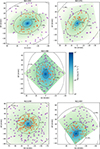 |
Fig. 1. PN sub-sample definitions for our galaxies. The orange circles represent the positions of the inner region PNe, and the purple squares denote the positions of the outer sub-sample. The galaxy surface brightness is logarithmically scaled in the same manner for all galaxies. Following Paper II, we exclude the inner 15″ of NGC 1399 as the PNe sample in that region is incomplete. |
For NGC 1052 and NGC 1399, we used the same datasets as in Paper II. NGC 1052 is a mosaic of two pointings from the same observing program, with a similar image quality of ∼0 6 and the same exposure time of 2788 seconds. The MUSE data of NGC 1399 is also a mosaic, but one constructed from five pointings with a range of seeing (0
 6 − 1
6 − 1 7) and exposure times (900 −1800 seconds) from two different programs. As discussed in Paper II, this mosaic was compromised by imperfect flat-field corrections and consequently, inconsistent noise levels. Following Paper II, we excluded the inner 15″, due to incompleteness caused by high surface brightness. For NGC 1351, NGC 1380, and NGC 1404, we only employed the single pointings close to the nucleus, where most of the PN candidates are located. We found that the nuclear pointings of these galaxies are sufficient to comply with our selection criteria.
The definition of the two PN sub-samples is based on the PNe’s isophotal galactocentric distance. First, we created synthetic R-band images from the MUSE datacube using the Python package synphot (Lim 2020). Using the images, we used photutils.isophote (Bradley et al. 2024) to define three ellipses with position angle PA and ellipticity ϵ: an inner ellipse with semi-major axis a1, within which PN detections are compromised by the galaxy’s high surface brightness, a middle ellipse with semi-major axis a2, which encloses half the observed PN population, and an outer ellipse a3, defined by the PN furthest from the nucleus. To convert the semi-major axes into effective radius units, we adopted Re from Forbes et al. (2017) for NGC 1052 and Iodice et al. (2019a) for the rest. These parameters are listed in Table 2 and illustrated in Fig. 1. The position angles and ellipticities are in good agreement with those found by previous surface photometry studies (Jedrzejewski et al. 1987; Iodice et al. 2019b).
Ellipse definitions for the PN sub-sample.
3. Fitting the PNLF
The apparent PN magnitude in the [O III]λ5007 line is defined as
 (1)
(1)
where F5007 is the flux of the [O III]λ5007 emission line in erg cm−2 s−1. We parametrized the shape of the cutoff to the PNLF using the analytic expression first given by Ciardullo et al. (1989); although more generalised expressions of the PNLF are available (e.g. Longobardi et al. 2013) this simple form is sufficient for our purposes. Briefly stated, we fit the PN magnitudes to
 (2)
(2)
where m* is the apparent magnitude of bright-end cutoff. These fits assume the Schlafly & Finkbeiner (2011) value for foreground Galactic extinction correction, use the published estimates of the galaxies’ surface brightness to obtain the luminosity function’s normalization factor, and adopt the position-dependent line-of-sight velocity dispersions to take into account the possibility of PN superpositions in the high surface brightness regions of the galaxies. A detailed description can be found in Chase et al. (2023). This results in a probability distribution function of two variables: the bright-end cutoff m* that can be converted into the galaxy’s true distance modulus (m − M)0 by assuming a value of M*, or vice versa, and the luminosity function’s normalization, α2.5. We note that to compute the values of the latter variable, we use an assumed V-band bolometric correction of BCV = −0.85 (Buzzoni et al. 2006); the α2.5 value is computed as the number of PNe within 2.5 mag of m* per unit bolometric luminosity of the sampled stellar population. However, for the relevance of distance determination, we are only interested in the PNe in the top 0.5 mag of the luminosity function, which define the PNLF cutoff. We therefore scale our observed α2.5 values to α0.5 following the recipe of Ciardullo et al. (2005) for our analysis.
For both the m* and α0.5 values, our errors account for the statistical errors of the fits only. Systematic uncertainties associated with the foreground reddening and the photometric zero-point of MUSE are not included. Radial dust distribution within the host galaxy can also affect the PNLF measurement, as shown in disk galaxy NGC253 (Congiu et al. 2025). However, since our sample consists of ETGs with typically low dust content and our analysis is mostly differential, comparing two regions within the same galaxy, the omission of these terms will not change our results.
4. Stellar population synthesis
4.1. Population models
We utilized the semi-empirical Medium-resolution Isaac Newton Telescope Library of Empirical Spectra (Knowles et al. 2021, sMILES;) simple stellar population (SSP) models (Knowles et al. 2023) to analyse the galactic spectra contained on the MUSE frames. The sMILES library uses as its basis the MILES empirical spectra (Sánchez-Blázquez et al. 2006; Falcón-Barroso et al. 2011), but includes fully theoretical corrections that allow for variations in the abundance of α-process elements, with [α/Fe] families of −0.2, 0.0, +0.2, +0.4, and +0.6 (Knowles et al. 2021). The library itself covers the wavelength range λλ3540.5 − 7409.6 Å at a spectral resolution of 2.51 Å. To calculate single stellar populations (SSP), Knowles et al. (2023) adopted solar scaled isochrones (Pietrinferni et al. 2004) for [α/Fe] = −0.2, 0.0, +0.2 and α-enhanced isochrones (Pietrinferni et al. 2006) for [α/Fe] = +0.4, +0.6. The models were computed in 10 metallicity steps [M/H] = −1.79, −1.49, −1.26, −0.96, −0.66, −0.35, −0.25, +0.06, +0.15, +0.26, as defined by Grevesse & Noels (1993), and 53 age steps between 0.03 and 14 Gyr. The SSPs are provided with five variations of the initial mass function (IMF); unimodal and bimodal from Vazdekis et al. (1996), universal and revised from Kroupa (2001), and from Chabrier (2003). For our analysis, we employed the universal Kroupa IMF.
As a consistency check, we also applied two other SSP models to our data. First, we tested the models from Vazdekis et al. (2015), that are based on the original MILES spectral library. These SSPs include [α/Fe] = 0.0, 0.4 models calculated using a correction factor obtained from a fully theoretical stellar library (Coelho et al. 2005, 2007). We note that in these models the abundance correction was applied to the SSP model spectra as a whole, in contrast to Knowles et al. (2023) where their corrections were applied to the individual star spectra before constructing the sMILES SSPs. Second, we also tested the semi-empirical model of Walcher et al. (2009), which used the theoretical library from Coelho et al. (2007) to correct their SSP fluxes as a function of [Fe/H] and [α/Fe]. Their base SSP models are adopted from Bruzual & Charlot (2003), Le Borgne et al. (2003), and Vazdekis (1999) and include ages between 2−13 Gyr, abundances of [Fe/H] = −0.5, −0.25, 0.0, 0.2, and [α/Fe] = 0.0, 0.2, 0.4. The model resolution is a constant FWHM = 1.0 Å. Detailed discussion on the comparison between different SSP models are presented in Appendix A.
4.2. SSP fitting
Our observational data consist of two integrated-light spectra for each galaxy: one for the system’s inner annulus and one for its outer annulus (as defined in Sect. 2). We fitted our observations to the SSP models using the Penalized Pixel-Fitting tool (pPXF; Cappellari & Emsellem 2004; Cappellari 2017, 2023), with the wavelength range limited to 4760 Å − 6800 Å to exclude sky lines in the redder part of the spectra. Additionally, we put masks centred on the telluric emission lines of [O I]λ5577.4, [O I]6300.3, and [O I]6363.7, Na Iλ5889.9, and O Iλ6157.5 (Guérou et al. 2016).
The MUSE line spread function (LSF) is a non-linear function of wavelength. For our fitting range, the LSF varies from FWHM = 2.46 to 2.77 Å. In contrast, the sMILES SSP models have a constant FWHM = 2.51 Å. For regions of the sMILES spectra with a LSF FHWM < 2.51 Å we did not apply any convolution to the SSP models; otherwise, we convolved the models with a kernel based on the LSF defined by Weilbacher et al. (2018),
 (3)
(3)
with the wavelength in Å. Then, to obtain the stellar population parameters, we applied the wild bootstrapping analysis (Davidson & Flachaire 2008; Cappellari 2023); a full description of this technique being applied to MUSE data using pPXF is given in Kacharov et al. (2018). In brief, we first performed an initial fit to obtain the residuals at each pixel. Then, we bootstrapped the data by resampling the residuals and refitting the spectrum 100 times. During this procedure, we applied a 12th order multiplicative polynomial to minimize any template mismatch and flux calibration errors, but we did not apply any additive polynomial correction as that might have biased the derived stellar population parameters (Guérou et al. 2016; Kacharov et al. 2018). Similarly, we did not apply any regularization for our measurements. Each of the 100 fits produced a luminosity-weighted measurement of the SSPs for different [M/H], [α/Fe], and ages. We took the averaged weights of the 100 fits and their standard deviation to be our light-weighted results. To obtain the mass-weighted values, we adopted mass predictions for the SSP models from Vazdekis et al. (2015) for the BaSTI isochrones (Pietrinferni et al. 2004, 2006). We calculated the mass-weights for each of the 100 luminosity-weights, before obtaining the average mass-weighted results and their uncertainties.
4.3. Star formation histories
Based on the SSP mass-weights, we constructed the history of mass assembly of the stellar population. As our aim is to investigate the parent population contributing to the PNe at the bright-end of the PNLF, we needed to define a coarse age range where these objects are expected. Based on the simulations of Valenzuela et al. (2019), central stars with masses in the range of 0.53 − 0.59 M⊙ are sufficient to reproduce the PNLF of the elliptical galaxy NGC 4697. This is further demonstrated by Valenzuela et al. (2025), who show which SSPs are capable of producing PNe at the bright cutoff (see their Fig. 10 for details).
The lifetimes and luminosities of the progenitor stars of [O III]λ5007-bright PNe depend on their initial mass, metallicity and helium abundance; thus it is important to constrain these variables. If we adopt the post-AGB models of Miller Bertolami (2016), stars with main sequence lifetimes > 10 Gyr will end up with central star masses of < 0.53 M⊙ and be too faint to excite an M* planetary. PN hydrodynamical simulations suggested that to produce PNe at the PNLF cutoff, a central star mass ≳0.58 M⊙ is necessary (Schönberner et al. 2007; Gesicki et al. 2018). The observation of PNLF cutoff PNe in M31 showed that the central stars have masses of 0.57 − 0.58 M⊙ (Galera-Rosillo et al. 2022; Morisset et al. 2023); the masses correspond to main sequence lifetimes of ∼2 − 3 Gyr. Recently, Valenzuela et al. (2025) found that, depending on the IFMR, the M* PNe can be formed by stellar populations as old as 10 Gyr at solar metallicity. Based on these considerations, we defined three age bins: t < 2 Gyr, 2 ≤ t ≤ 10 Gyr, and t > 10 Gyr to derive the stellar mass fractions and investigate the progenitor population of our PNe. We note that these definitions are dependent on the populations model, in this case the sMILES SSPs.
5. Simulation analogues
To interpret the relationship between the bright-end of the PNLF and underlying stellar populations, we apply PNe In Cosmological Simulations (PICS; Valenzuela et al. 2025) in post-processing to the Magneticum Pathfinder1 simulation Box4 ultra-high resolution (uhr). This cosmological hydrodynamical simulation, which was run with GADGET-3, a modified version of the GADGET-2 code (Springel 2005), has a box side length of 68 Mpc, an average stellar particle mass of ⟨m*⟩ = 1.8 × 10⁶ M⊙ and a softening length of ϵ* = 1 kpc; for more details about the implementation and set-up, see Teklu et al. (2015), Dolag et al. (2025). Galaxies and their sub-structures are identified with the subhalo finder SUBFIND (Springel et al. 2001; Dolag et al. 2009). In the simulation volume roughly 700 galaxies with stellar masses above M★ ≈ 2 × 10¹⁰ M⊙ are formed by z = 0. The galaxies of Box4 (uhr) have been analysed in numerous studies and have been shown to agree well with observations in a multitude of properties. An overview of these studies can be found in Sect. 2.1 of Valenzuela et al. (2024). One caveat to note about the Box4 simulation is that the run only reaches z ≈ 0.066, which corresponds to a look-back time of around 0.88 Gyr. For this reason, the stellar ages reach a maximum of 12.9 Gyr.
For the selection, we do this matching as closely as possible: morphological type (here, either elliptical or lenticular), effective radius (as reported by Forbes et al. 2017 and Iodice et al. 2019a assuming the distances of Jacoby et al. 2024), and g − r colour (Persson et al. 1979; Iodice et al. 2019b)2. Specifically, we began by discarding all simulated galaxies classified as late-type by their dynamical morphology indicator (the b value; Teklu et al. 2015) according to the classification scheme employed by Valenzuela & Remus (2024). Next, we excluded systems whose effective radii differed by more than 30% from their observed counterparts, or more than ±0.4 from the observed g − r colour. Finally, we identified the most suitable galaxies in the Magneticum simulation via the metric
 (4)
(4)
where the galaxies with the lowest values of m were taken as analogues. Only duplicate analogues for two different observed galaxies are skipped. Due to the limited size of the simulation box, we are limited to a low number of galaxies. In the end, we selected six analogue galaxies for each of our five observed objects. We find that six galaxies give a compromise between not being bound to a single analogue object and not deviating too much from our selection parameters.
For each of the galaxy analogues, we ran the fiducial PICS model on each stellar particle belonging to its respective galaxy; this results in set of PNe, with a position and a M5007 magnitude. The PICS procedure is as follows. As input, PICS takes a single stellar population with a given age, metallicity mass fraction, total mass and initial mass function (IMF). From the age, the number of stars now entering the post-AGB phase are determined through the lifetime function (Miller Bertolami 2016), the total mass and IMF. Each post-AGB object is then assigned a core mass through the Miller Bertolami (2016) initial-to-final mass relation (IFMR), and then a stellar luminosity and effective temperature using the Miller Bertolami (2016) evolutionary tracks and a randomly drawn post-AGB age. We note that the lifetime function, IFMR, and post-AGB tracks are all metallicity-dependent. Based on the central star properties and post-AGB age, the intrinsic M5007 magnitude is obtained from the nebular model of Valenzuela et al. (2019) corrected for metallicity according to Dopita et al. (1992). Finally, the actually measured magnitude is obtained by applying the circumnebular extinction relation by Jacoby & Ciardullo (2025). For more details on the PICS model, see Valenzuela et al. (2025).
To obtain the PNe in analogues radial bins to the observations, we used the values given in Table 2 for a1, a2, and a3 and converted them to kpc according to the respective PNLF distances. We then viewed the simulated galaxy from a random direction, and, using the ellipticities listed in Table 2, defined its inner and outer annulus in a manner similar to that of the observed galaxy. The PNe found in the simulation’s projected regions then serve as the comparison sample for the observed PNe.
The analogue galaxies function as hosts of PN populations with self-consistent cosmological star formation histories, which we can compare to observations. This allows us to gain a deeper understanding of the underlying processes and how galaxy properties are related to their PN population. This, in turn can be compared to the observational findings. However, we note that none of the simulated galaxies are exact replicas of the observed systems nor were they produced under constraints to reproduce the program galaxies. Thus, the comparisons may not be perfect.
6. Results
6.1. PNLF and stellar populations
6.1.1. NGC 1052
NGC 1052 is a bright elliptical galaxy with a LINER-type nucleus which is known to have X-ray variability (Dopita et al. 2015; Osorio-Clavijo et al. 2020). A total of 86 PNe were identified in Paper II, giving us 43 PNe per ellipse region. To measure the distance modulus, we adopted the R-band surface brightness photometry from Jedrzejewski et al. (1987), used the velocity dispersion data of Binney et al. (1990), and assumed a population (V − R) = 0.93 colour (Persson et al. 1979) with E(B − V) = 0.023 (Schlafly & Finkbeiner 2011). For the inner annulus, we estimated the limiting PN magnitude for 90% completeness to be m5007 = 27.6, while in the outer annulus, the galaxy’s lower surface brightness enabled measurements to m5007 = 27.8. The completeness is estimated at the point where the PNLF deviates from the analytical function. Based on experience, while the selection of bin sizes might impact the completeness limit, and an artificial star experiment may improve it, our estimation is sufficient for our purpose. The PNLFs are shown in Fig. 2.
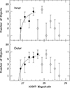 |
Fig. 2. PNLFs of the inner and outer region of NGC 1052, binned in 0.2 mag intervals. The solid and open points represent data brighter than and fainter than the completeness limit, respectively. The curves show the analytic PNLF, shifted using the most likely apparent distance modulus and normalization. |
Fit parameters for NGC 1052.
The fitted parameters are shown in Table 3. The difference between the PNLF cutoff between the two regions is  . The PN density in both annuli is similar with
  . Both regions are very old, with average weighted ages greater than 12 Gyr. The inner region appears more metal-rich than the outer by ∼0.1 dex, while the difference in [α/Fe] is not as significant. The errors in the age fraction are generally high due to the uncertainties in the fitting process. Regardless, our results are generally in agreement with previous studies of NGC 1052 that found an older and more metallic population in the inner part of the galaxy (Raimann et al. 2001; Milone et al. 2007; Dahmer-Hahn et al. 2019).
6.1.2. NGC 1351
NGC 1351 is a peculiar lenticular galaxy (Hubble type SA0; de Vaucouleurs et al. 1991)  from the centre of the Fornax Cluster. In Paper II, 102 PNe were found, but as explained in Sect. 2, for this differential analysis we only use the PN detections in the MUSE pointing centred on the nucleus. This gives us a total sample of 86 PNe. Our surface photometry data came from the B-band observations of de Carvalho et al. (1991), which was then converted to V using (B − V) = 0.90 (Faber et al. 1989) and E(B − V) = 0.016 (Schlafly & Finkbeiner 2011). These data yield V = 14.23 for the light contained in our inner annulus and V = 14.65 for light of the outer annulus. The line-of-sight velocity dispersion underlying each PN was estimated from the data presented by D’Onofrio et al. (1995).
We assume our measurements to be complete to m5007 = 28.0 in the galaxy’s high surface brightness inner annulus, and m5007 = 28.5 at the inner and outer annulus; our exact choice of limiting magnitude has no effect on the derived distance and only a minor effect on the PN density. The PNLF plots are shown in Fig. 3 and the parameters from our analysis are presented in Table 4. We note that we exclude one, apparently overluminous PN in the outer annulus of the galaxy; this object is fully discussed in Paper II.
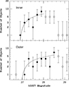 |
Fig. 3. PNLFs of the inner and outer regions of NGC 1351, binned in 0.2 mag intervals. The solid and open points represent data brighter than and fainter than the completeness limit, respectively. One overluminous PN was excluded from the outer PN sample; that object is also shown as an open circle. The curves show the analytic PNLF, shifted using the most likely apparent distance modulus and normalization. |
Fit parameters for NGC 1351.
Between the two regions, the difference in the PNLF cutoff is an insignificant  . Similarly, the PN densities within the two regions are also consistent, with
  . The inner and outer region have mean weighted ages of ∼11 Gyr and ∼9 Gyr, respectively. The total metallicity in the inner annulus is [M/H]∼ − 0.3, which is ∼0.1 dex more metal rich than the outer annulus but within the uncertainties. The [α/Fe] of the two regions are not significantly different. Compared with the stellar population calculation of Iodice et al. (2019a), we have younger ages by ∼1 − 2 Gyr and lower total metallicity. We argue that this is due to the model dependence of the SSP fitting as the latter study employed the older MILES SSPs; support for this in given in Appendix A. Nevertheless, the overall radial trends for our stellar population parameters are in an agreement.
6.1.3. NGC 1380
NGC 1380 is another lenticular (SA0) galaxy in the Fornax cluster. It was one of the benchmark galaxy for the demonstration of the DELF method of MUSE reduction (Paper I), and has been the subject of numerous analyses, in part because of its well-observed Type Ia supernova 1992A. In particular, studies of the galaxy’s stellar initial mass function, kinematics, and gas components have been performed as part of the Fornax3D project (Sarzi et al. 2018; Iodice et al. 2019a; Martín-Navarro et al. 2019; Viaene et al. 2019).
In Paper I, 166 PNe were identified in three MUSE pointings; 112 of these are present in the nucleus data cube. Our PNLF analysis uses the ugri surface photometry of Iodice et al. (2019b), which was converted to the V-band using the transformations given by Lupton (2005), and a foreground extinction value of E(B − V) = 0.015 (Schlafly & Finkbeiner 2011). This yielded V = 11.88 for the galaxy’s inner annulus and V = 11.92 for our outer annulus. The line-of-sight kinematics underlying each PN were found from Iodice et al. (2019a).
The luminosity functions are shown in Fig. 4. We assume a limiting magnitude of m5007 = 27.7 and m5007 = 27.9 for the inner and outer annulus, respectively. The PNLF fit and stellar population parameters are presented in Table 5. Once again, we excluded one PN candidate that is overluminous compared to the rest of the population in the outer annulus; see Paper I for details.
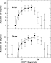 |
Fig. 4. PNLFs of the inner and outer region of NGC 1380, binned in 0.2 mag intervals. The solid and open points represent PN bins brighter than and fainter than the completeness limit, respectively. One overluminous PN was excluded from the outer PNLF sample, and is shown as an open circle. The curves show the analytic PNLF, shifted using the most likely apparent distance modulus and normalization. |
Fit parameters for NGC 1380.
The PNe of the inner annulus of NGC 1380 exhibits a brighter PNLF cutoff ( ) and a lower PN density (
 ) than their outer annulus counterparts, but neither offset is significant. The average weighted stellar age is ∼12 − 13 Gyr. The inner annulus exhibits solar metallicity, while the stars in the outer annulus are sub-solar with [M/H]∼ − 0.10. There is no significant difference in [α/Fe] between the regions. Our values are in agreement with the measurements by Iodice et al. (2019a) and Martín-Navarro et al. (2019). With respect to the latter, we note that they have explored the variability of the initial mass function in this galaxy, which we did not take account for.
6.1.4. NGC 1399
NGC 1399 is the dominant cD/elliptical galaxy of the Fornax cluster, and, due to its mass and MUSE coverage, it has more detected PNe than any other galaxy in Paper II. The first observations of PN in the elliptical galaxy NGC 1399 date back to the multi-object spectroscopy with the ESO NTT by Arnaboldi et al. (1994). Follow-up observations with the ESO FORS spectrograph in counter-dispersed slit-less spectroscopy detected 146 PNe covering a radial range in the outer halo from 100″ to 500″ (McNeil et al. 2010).
For the current investigation of the PNLF properties we restrict ourselves to the central regions of NGC 1399 sampled with MUSE. As in Paper II, we excluded all PNe within 15″ of the galaxy’s nucleus as detections in this region are compromised by the bright, rapidly varying background. The galaxy’s surface brightness distribution has been measured several times at different depths and scales (Franx et al. 1989; Caon et al. 1994; Iodice et al. 2016); in our analysis, we combined these data with an assumed E(B − V) = 0.011 (Schlafly & Finkbeiner 2011) to create the galaxy’s V-band surface brightness profile. The line-of-sight velocity dispersion is adopted from (Saglia et al. 2000). Outside of this region, we used a common limiting magnitude of m5007 = 28.0. Using the galaxy’s V-band surface brightness distribution, we calculate that our inner annulus of PNe contains V = 11.13 of total light, while the outer annulus encompasses V = 11.40. Our measured luminosity functions are shown in Fig. 5.
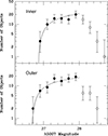 |
Fig. 5. PNLFs of the inner and outer region of NGC 1399, binned in 0.2 mag intervals. The solid and open data points represent data brighter than and fainter than the completeness limit, respectively. The curves show the analytic PNLF, shifted using the most likely apparent distance modulus and normalization. |
Fit parameters for NGC 1399.
The fitted parameters for the PNLF and stellar populations are given in Table 6. Compared to the PNe in the outer annulus of the galaxy, the PNe in the inner annulus have a PN density that is lower by  , and a cutoff magnitude that is fainter by
  ; both offsets are intriguing, but not definitive. In contrast, our stellar population fits show that both annuli have similar average weighted ages and [M/H] values. The [α/Fe] estimate for the outer annulus is larger than that of the inner region, but still within their uncertainties. These stellar population trends are consistent with the findings of Vaughan et al. (2018).
6.1.5. NGC 1404
This galaxy is located about 10 arcmin from the centre of NGC 1399. The counter-dispersed slit-less spectroscopy observations of NGC 1404 by McNeil et al. (2010) provided 23 PNe associated with the light of NGC 1404. On the basis of a Gaussian Mixture Model decomposition of the line-of-sight (LOS) velocity distribution, it shows the different LOS systemic velocity between NGC 1404 (1933 kms−1) and NGC 1399 (1425 kms−1).
Again, for the current investigation of the PNLF properties, we restrict ourselves to the central regions of NGC 1404 sampled with MUSE. In Paper II, a total of 126 PN candidates were identified, with 107 PNe in the MUSE pointing that we study here. This gives us 54 and 53 PN samples for the inner and the outer annulus, respectively.
To derive the PNLF, we employed the R-band surface photometry of Franx et al. (1989), converted it to the V-band using a colour of (V − R) = 0.38 (Muñoz-Mateos et al. 2009), and adopted a foreground extinction of E(B − V) = 0.010 (Schlafly & Finkbeiner 2011). Our information about the line-of-sight velocity dispersion came from D’Onofrio et al. (1995) and Iodice et al. (2019b). For the inner annulus, we calculated a V-band magnitude of V = 10.81 and assumed a completeness limit of m5007 = 27.8. For the lower surface brightness outer annulus, V = 12.17 and a completeness limit reaches m5007 = 28.2. The PNLF of the two sub-samples in NGC 1404 can be seen in Fig. 6. The fitted parameter for the PNLF cutoff and the stellar population are presented in Table 7.
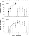 |
Fig. 6. PNLFs of the inner and outer region of NGC 1404, binned in 0.2 mag intervals. The solid and open data points represent data brighter than and fainter than the completeness limit, respectively. The curves show the analytic PNLF, shifted using the most likely apparent distance modulus and normalization. |
Fit parameters for NGC 1404.
We see no significant shift in the PNLF cutoff magnitude between the two populations with  . The PN density in the outer annulus is larger by
  , but, as indicated by the uncertainties, this difference is, at best, marginally significant. The stellar population trends for the age and abundances of each regions are also in agreement with the results of Iodice et al. (2019a). Both annuli exhibit an old population with the average weighted age of 12 − 13 Gyr. This is also shown by the large fraction (∼97%) of old stars in the galaxy’s star formation history. The remaining fraction of ∼2% in the inner annulus is dominated by stars younger than 2 Gyr, while in the outer annulus, this population has intermediate ages between 2–10 Gyr.
6.1.6. Observation summary
We have measured the PNLFs and stellar populations in ten regions within five galaxies. Although the Δm* and Δα0.5 between regions within a single galaxy may not be significant, a combinations of all the result will allow us to investigate whether there are significant correlations between the PNLF parameters and the stellar population parameters. We discuss this in detail in Sect. 7.1 and Sect. 7.2. For the stellar population discussions, we only consider the mass-weighted values.
6.2. Simulated analogue galaxies
The stellar population parameters of our galaxies’ analogues are shown in Table 8, and compared to observations in Fig. 7. The [α/Fe] abundance ratio is not given in the simulations. The ages of our analogues are 20 − 40% younger than those derived from the observations, except for NGC 1351, where the values are consistent. For total metallicities, both dataset are generally in a good agreement, with NGC 1351 again being an outlier. In our observations, we find that the inner annuli have ∼0.12 dex higher metallicity on average than the outer. On the other hand, for the simulation analogues, the inner annuli are ∼0.06 dex more metal rich on average than the outer annuli, with a larger scatter. For the age gradient, both the observations and simulations have a negligible difference on average, with the simulations having smaller scatter. Considering their weighted averages and uncertainties, both of the datasets sit in a similar region in the Δ[M/H]−ΔAge diagram. Therefore, assuming that the age and metallicity are the main influence to the PN population, we are confident in using the simulation analogues as an additional tool to interpret our observations. We will use the predicted value of the M* and the luminosity-specific PN number from PICS to test whether the observed trends are in agreement with the current theoretical understanding.
Stellar population age and [M/H] of the simulated analogue galaxies.
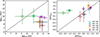 |
Fig. 7. Comparison of the stellar population age (left) and total metallicity (right) between the observations and the simulations. The solid and open markers indicate the inner and outer annulus, respectively. The dashed line indicates the one-to-one comparison. |
7. Discussion
7.1. Stellar population dependence on M*
To examine the effect of stellar population on the absolute PNLF bright-end cutoff, M*, we tested three approaches. First, we converted the observational values of m* into M*, assuming distances from different techniques: PNLF, SBF, and TRGB. The zero-points between these techniques are known to be discrepant (Ciardullo et al. 2002; Ciardullo 2012), and we want to investigate whether it is related to the stellar population. The second approach is from the theoretical perspective, to track the expected behaviour of M* in our simulated analogue galaxies with different stellar populations. Thirdly, we make differential comparisons of M* between the inner and outer annulus of the observation and simulation data. In other words, we trace the behaviour of M* to the radial changes of the stellar population in each galaxy. This last analysis is differential in nature, and therefore does not require knowledge of the galaxies’ of a true distance.
7.1.1. M* from different distance methods
We calculated M* using three different distances: the PNLF measurements from Papers I and II, the SBF values from Blakeslee et al. (2009) and Tonry et al. (2001), and the TRGB distances for NGC 1380, 1399, and 1404 (Anand et al. 2024b). Currently, there are no TRGB distances to NGC 1351 and NGC 1052; although TRGB has been measured in the dwarf satellite galaxies NGC 1052-DF2 (van Dokkum et al. 2018) and NGC 1052-DF4 (Danieli et al. 2020), we have opted not to use these measurements. The adopted distances are tabulated in Appendix B.
A comparison of the relation between M* and population age and metallicity for the three distance methods is presented in Fig. 9. The M* uncertainties are propagated from the statistical fit of the m* and the distance moduli. The weighted average of the bright-end cutoff using the PNLF distances is M* = −4.52 ± 0.12, which is unsurprisingly consistent with the assumed M* = −4.53 and M* = −4.54 in Papers I and II, respectively. We use this value as a reference point for the comparison with the M* values derived from the SBF and the TRGB distances.
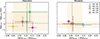 |
Fig. 8. Age and metallicity differences between the inner and outer regions of each observed galaxies (left) and the simulation analogues (right). The dot-dashed lines and the highlights indicate the weighted average and standard deviation, respectively. |
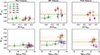 |
Fig. 9. M* derived using three distance determination methods: PNLF, SBF, and TRGB. The PNLF method assumes M* = −4.54 and acts as a reference point for this comparison. The dot-dashed lines indicate the weighted average. The solid and open markers denote the inner and outer annulus, respectively. The highlights indicate the standard deviation. |
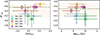 |
Fig. 10. M* from our simulation analogues as a function of total metallicity (left) and age (right). The dot-dashed lines indicate the weighted average. The solid and open markers represent the inner and outer annuli, respectively. The highlights illustrate the standard deviation. We note that the x- and y-axis ranges are different to those in Fig. 9. |
The SBF distances give a weighted average of  , which is 0.25 mag brighter than the typically assumed cutoff magnitude. The discrepancy is consistent with the known zero-point offset between the SBF and the PNLF distance scales (Ciardullo et al. 2002; Ciardullo 2012). SBF distances tend to have ∼0.2 mag larger distance modulus than the PNLF measurements, possibly because of a combination of minor systematic errors associated with both methods that work in opposite directions (Ciardullo 2012). The TRGB comparison also yields a PNLF cutoff that is brighter than expectations (
 ), though the nominal value is still within the uncertainties. We note that the I-band TRGB measurement typically requires a population with a metallicity [Fe/H] ≲ 0.7; otherwise the effect of line-blanketing on the RGB stars is non-negligible, necessitating a metallicity correction (Bellazzini et al. 2001; Ciardullo et al. 2002; Rizzi et al. 2007). To minimize this effect, Anand et al. (2024b) did select their fields to be in the galaxies’ outer regions. However, some line-blanketing issues may still be present.
Although solving the discrepancies between the PNLF, SBF, and TRGB distance scales is beyond our scope of this paper, we can still address whether metallicity or age differences have a significant effect on M*. We note that we only have one galaxy with a substantial population of stars with ages < 12 Gyr and [M/H]< − 0.2, we find that over the metallicity range −0.4 ≲ [M/H] ≲ +0.2 and the age range of 9 to 13.5 Gyr, M* does not show any trends regardless of the calibration technique. This shows that the zero-point discrepancies between the techniques are not related to the stellar populations age nor metallicity. In their analysis of the PNLF zero-point, Dopita et al. (1992), Schönberner et al. (2010) found that the zero-point discrepancy of the PNLF between Cepheid distance scales should be independent of age and metallicity, which is in agreement with our findings.
7.1.2. M* from simulated analogue galaxies
We investigate if a correlation exists between M*, age, and [M/H] for the simulated galaxies plotted in Fig. 10. Here, the M* uncertainties are the standard deviation between the six analogue galaxies representing each of the observed galaxy. The analogues of NGC 1052 and NGC 1351 have the largest scatter with brightnesses up to ∼0.3 mag fainter than the canonical M* = −4.54 value. Individual analogues with a combination of old (≳10 Gyr) and metal-poor ([M/H]≲ − 0.1) tend to produce PN populations with M* ∼ −4.0. On the other hand, when the stellar populations are either younger or more metal rich, the PN populations can exhibit a PNLF cutoff much brighter than M* ∼ −4.5. Since some analogues for these two galaxies fall into the earlier category, they should have larger scatter on average. Overall, the simulated galaxies have the weighted average of  . We also calculated the weighted average if the two galaxies with the largest scatter are excluded; in that case
  . Nevertheless, we also do not find any correlation between M* and age and metallicity for our simulation data.
7.1.3. M* from stellar population gradient
We now make a differential comparison between the inner and outer annulus of the observations (Δm*) and that of the simulation data. In this approach, the adopted distance to each of the galaxies is irrelevant and therefore Δm* = ΔM*. This comparison is presented in Fig. 11. In both datasets, we find that M* is almost identical for the existing age and metallicity gradient within each galaxy. Specifically, we measure a weighted average of  for the observations and
  for the simulations. In this approach, the stellar population parameters also show a negligible effect on M*. We note that the large M* uncertainties of the observations stem from the statistical errors on the PNLF fits, while the M* uncertainties associated with the simulations represent the standard deviation from the individual simulated analogue galaxies selected for each observed galaxy.
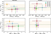 |
Fig. 11. Inner annulus minus outer annulus difference in M* vs. that for metallicity and age for the observations (left) and simulation analogues (right). The dot-dashed lines indicate the weighted average. The highlights show the standard deviation. |
In low-metallicity systems, Ciardullo et al. (2002) showed that M* is sensitive to the oxygen abundance and could be up to ∼0.2 mag fainter. For example, in the different populations of M31, Bhattacharya et al. (2021) presented the behaviour of M* as a function of metallicity and showed that between −0.6 ≲ [M/H] ≲ −0.4, the PNLF cutoff can be fainter by up to ∼1.0 mag, and reach M* ≃ −2.7 at [M/H] ≃ −1.1. However, when [M/H] > −0.4, the PNLF cutoff is expected to stay constant at M* ∼ −4.5. A possible fainter M* due to metallicity has also been observed in M49 (Hartke et al. 2017). Support for this comes from Paper II, where the PNLF cutoff of the galaxy’s inner regions was found to be ∼0.4 mag brighter than that derived by Hartke et al. (2017) from narrow-band observations of the galaxy’s outer envelope and halo.
Our findings of negligible radial metallicity dependence in our sample fit into the picture. Since our galaxies have metallicity [M/H] > −0.4, any significant metallicity effect seems unlikely. On the other hand, for populations with super-solar metallicities, Dopita et al. (1992) predicted a decrease in M*, which at first glance appears to contradict our results. However, in such systems, there will always be enough stars at solar-type metallicities to produce PNe with M* ∼ −4.5. Hence no shift in M* should be observable (see Paper II and Ciardullo et al. 2002).
7.1.4. Conditions for a constant M*
Based on our analysis using different approaches, despite our limited sample, we are convinced that the independence of M* from the stellar population can always be achieved with an appropriate target selection. To elaborate this, we look into the mass-metallicity relationship (MZR) of galaxies. The stellar masses of our ETGs are in the range of 10.33 ≲ log M★/M⊙ ≲ 11.44 (Iodice et al. 2019b). Using SDSS, Gallazzi et al. (2006) showed that ETGs with log M★/M⊙ ≳ 10 are likely to have metallicities of [M/H] ≳ −0.2. This is also supported by the MZR for z = 0 galaxies in the Magneticum simulations (Kudritzki et al. 2021; Dolag et al. 2025). We did not analyse any star-forming galaxies in this work, but the assumption of a constant PNLF cutoff is also expected to hold for those galaxies. Although their MZR slope is different from that found for quiescent galaxies (Gallazzi et al. 2014), we still expect massive star-forming galaxies to be relatively metal-rich. Specifically, for star-forming galaxies with stellar mass log M★/M⊙ ≳ 10, we expect [M/H] ≳ −0.1 (Bresolin et al. 2022; Urbaneja et al. 2023; Sextl et al. 2023, 2024). The scatter of [M/H] in these MZRs is typically ∼0.1 dex.
Based on the MZR, metal-poor galaxies with [M/H] ≲ −0.4 will have low stellar masses, and only a few PNe in the top magnitude of the luminosity function. Since precision PNLF distances require ≳30 PNe in this magnitude range (Papers I and II), their selection in the context of the Hubble constant measurement should be avoided. If distances were derived from outer halo populations, where the stellar population are metal-poor (Longobardi et al. 2015; Hartke et al. 2017, 2020), a (possibly uncertain) metallicity correction may be necessary (Ciardullo et al. 2002). To minimize these systematic errors, the ideal targets for PNLF-H0 investigations are the inner regions of massive galaxies, where the abundance-based shifts in M* are negligible.
7.2. PN numbers at the PNLF cutoff
We investigate how the stellar population affects the luminosity-specific PN number, otherwise known as the α-parameter, at the PNLF cutoff. Typically, this parameter is defined as α2.5, which represents the number of PNe within 2.5 mag of the cutoff per unit bolometric luminosity of the surveyed galaxy, is particularly important as a probe of the underlying stellar population (Buzzoni et al. 2006; Longobardi et al. 2013; Hartke et al. 2017, 2020). However, as explained in Sect. 3, we are only interested in PN density at the top 0.5 mag of the luminosity function (α0.5). For the simulation data, the α0.5 values are obtained directly from the simulation. We discuss its dependence on age, [M/H] and [α/Fe].
Linear fit parameters between α0.5 and mass fraction of different ages.
Linear fit parameters of α0.5 with [M/H] and [α/Fe].
7.2.1. Age dependence
We compare the α0.5 values of different age groups in Fig. 12. As explained in Sect. 4.3, we defined these age groups based on the core mass predictions for the PNe. Overall, α0.5 found from the observations are smaller than those observed in the simulations. However the trends are similar. We tested whether the correlations between α0.5 and the mass fractions of different age groups are significant using Pearson correlation statistics with scipy.stats.pearsonr (Kowalski 1972). Then, we fitted a linear function y = c1x + c2 to the data using orthogonal distance regression with scipy.odr.odr (Brown & Fuller 1990). We fitted the data twice for the observation, with and without NGC 1351. The fit parameter results are presented in Table 9.
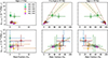 |
Fig. 12. Galaxy α0.5 values as a function of the mass fraction of young (Age < 2 Gyr), intermediate (2 ≥ Age ≥ 10 Gyr), and old (Age > 10 Gyr) stars. Upper panels: Observations. Lower panels: Values from the simulations. The green dot-dashed lines show the best-fit regressions; fits that exclude the observational data for NGC 1351 are shown as a brown dashed line. |
Both observation and simulations contain ≲5% mass fractions for stars younger than 2 Gyr. In neither do we see any correlation between the young population and α0.5. The p-values for the young populations are 0.76 and 0.84 for the observations and simulations, respectively; we skipped the fitting process due to the non-correlation. For the intermediate age population, we found a positive linear correlation for both the observations and the simulations, though the correlation for the observations weakens when NGC 1351 is excluded. Although the slope derived from the observation is steeper than that predicted from the models, the main indication is that more bright PNe will be formed when the mass fraction of the intermediate age population is larger. This is in agreement with Valenzuela et al. (2019, 2025), who predicted most PNe observed at the bright-end of the PNLF have main sequence lifetimes between 2 and 10 Gyr. Moreover, we found a negative correlation when comparing α0.5 to the > 10 Gyr stellar population.
These findings imply a relationship between PN core-mass and α0.5. The PN formation rate per luminosity unit is rather insensitive of age (Renzini & Buzzoni 1986; Buzzoni et al. 2006). However, the visibility timescale of a PN at its [O III]λ5007-bright phase depends strongly on the mass of its central star, and this mass, in turn depends on the progenitor’s initial mass and therefore lifetime. As a result, PN visibility depends critically on the inverse of population age, and this largely defines α0.5. For example, when the population is very young (< 2 Gyr), the PN [O III]λ5007-bright phase timescale will be very short, and theoretically should make the α0.5 smaller; this trend is not visible in our ETGs, possibly because all of our samples exhibit similar mass fraction of the very young populations. The positive trend for the intermediate ages show that an older population in this age range create PNe with lower core mass, which evolve slower, and therefore stay visible longer; giving higher α0.5 values. For the old populations (> 10 Gyr), a different condition occurs. While the lifetimes of these stars are the longest, a core-mass of ≲0.53 M⊙ simply do not produce enough luminosity to produce ≳400 L⊙ of [O III]λ5007 emission (Valenzuela et al. 2019). Hence, the α-parameter will decrease if the fraction of old population increases.
7.2.2. [M/H] and [α/Fe] dependence
We also analysed the trend of α0.5 with respect to metallicity. For the observations, we looked into correlation with both [M/H] and [α/Fe]; for the simulations, we only examined [M/H], since no information on the α-process to iron ratio was available. We tested the correlations and fitted the data similarly with the age fractions. The relations are presented in Fig. 13 and the fitted parameters are listed in Table 10. We find an anti-correlation between α0.5 and [M/H] in both datasets, but a positive correlation between α0.5 and [α/Fe]. This is expected, because in ETGs, [M/H] and [α/Fe] are anti-correlated (Walcher et al. 2015). However, we note that the correlation with [M/H] relies on NGC 1351: if that galaxy is excluded, the result is no longer significant.
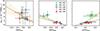 |
Fig. 13. Left and middle: Our α0.5 measurements as a function of [M/H] for the simulations and observations, respectively. Right: Our calculated [α/Fe] values for the observations. The green dot-dashed lines show our best fit regressions; fits that exclude NGC 1351 are denoted by the dashed brown line. |
Previously, Ciardullo et al. (2005) investigated the metallicity dependence of α0.5 using the [MgFe] line indices and found no strong trend. Similarly, in their MUSE study of edge-on galaxies in Fornax, Galán-de Anta et al. (2021) measured the α2.5–[M/H] relationship via two different methods: full spectral fitting and single-age population fits focused on specific line indices. They also found an anti-correlation of α2.5 with [M/H] but no trend versus the line indices. They speculated that the discrepancy might be caused by the variation in [α/Fe]. We speculate that the enrichment of alpha elements, which also includes oxygen, plays a role in the production efficiency of PNe at the PNLF cutoff. Assuming our derived trend which includes NGC 1351 is accurate, one could have a factor of ∼3 − 5 times more PNe at the top 0.5 mag of the PNLF for a system with [M/H] = −1.0. This prediction aligns to the findings of high α-parameters in outer haloes of ETGs, where the metallicity is expected to be low (Longobardi et al. 2013, 2015; Hartke et al. 2017, 2020). In the metallicity range where the M* can be assumed as constant, i.e. the central Re of ETGs, α0.5 should be relatively constant and only vary by a factor of ≲2.
7.3. PN progenitors at the PNLF cutoff
From the α0.5 values, we can also estimate the fraction of stars that turned into the PNe at the top 0.5 mag of the PNLF (f0.5). Based on the fuel-consumption theorem (Renzini & Buzzoni 1986; Buzzoni et al. 2006),
 (5)
(5)
where B is the bolometric luminosity-specific stellar evolutionary flux and t is the visibility lifetime of the PN-phase when M* is at its maximum. For all PN-forming stellar populations B ≃ 2 × 10⁻¹¹ stars yr−1 L⊙−1, with a minor dependency on age and IMF. Based on post-AGB evolution models (Miller Bertolami 2016), cores bright enough to excite a PN within 0.5 mag of M* (∼0.58 to 0.62 M⊙), only have visibility timescales of 500 to 1500 years (e.g. Schönberner et al. 2007; Gesicki et al. 2018). If we adopt 1000 years for this [O III]λ5007-bright phase, then we can compare f0.5 to the mass fraction of a galaxy’s stars that are younger than 10 Gyr (f< 10Gyr). We combine the young and intermediate-age stellar population because both can theoretically produce PNe in the top 0.5 mag of the luminosity function (Valenzuela et al. 2019, 2025). The comparison is shown in Fig. 14.
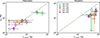 |
Fig. 14. Production efficiency for PNe within 0.5 mag of M* vs. the mass fraction of stars with ages less than 10 Gyr for the five galaxies in our survey. Left: Observations data. Right: Predictions from the simulated galaxies. The arrows indicate uncertainties that reach values of less than 1%. |
Despite the large uncertainties from the stellar population synthesis, our assumptions produce an almost one-to-one relation between the fraction of stars derived from the fuel-consumption theory and that inferred from the galaxies’ young and intermediate-age stellar populations. This seems to imply that the ETGs have enough young and intermediate-mass stars to produce the PNe seen in the top 0.5 mag of the PNLF. However, there is more to the story. We assume PN formation efficiencies at the top 0.5 mag using
 (6)
(6)
Our observations imply a median efficiency of 90 ± 40%; such a high efficiency is rather unlikely. For example, when we apply our simple assumptions to the simulations, we predict that only 35 ± 10% of the stars turned into the [O III]λ5007-bright PNe. Moreover, we argue that even this number is already an overestimation for two main reasons: (1) the simulations currently predict more PNe than the observations, and (2) the core masses obtained from the simulations have a median mass of 0.55 M⊙; such a low mass implies a visibility timescale that is almost an order of magnitude longer than that assumed. Thus, through Eq. 5, f0.5 and therefore the actual PN production efficiency must be much less than 35%.
There are several arguments to explain the discrepancy between our calculated value of 90% efficiency, and the expectations that the number should be of the order of ∼10%. Firstly, if the fraction of a given population is small (say, less than 5%), then the uncertainty in the measurement is generally quite large, typically between 50% and 370%. The detection of such a small population is very challenging and the results propagate directly into the efficiency predictions. At the extreme, it could reduce the efficiency down to ∼20%.
Secondly, the assumed visibility timescale of 1000 years is based on post-AGB models for stellar population age of ∼1 Gyr (Gesicki et al. 2018). If older populations also produce M* PNe, then the mean visibility timescale of the observed PNe will be longer. In fact, a small difference in the age of the assumed PN population could easily change the timescale by a factor of two, and this error would immediately propagate into calculated efficiency. Similarly, the assumed age population also effects B. Although the luminosity specific stellar evolution flux, is relatively independent of stellar population, changes in age and IMF can shift its value by 10 − 20%. Again, this change propagates directly into the efficiency estimate.
Regardless of the true value of ηPN, 0.5, the linear relationships between f0.5 and f< 10Gyr in both observations and simulations has an important implication on the PN formation mechanism in old stellar systems. Previously, it was thought that a population of ∼1 Gyr was needed to form M* PNe. Since the fraction of such stars in ETGs is extremely low, other evolutionary channels were invoked. These included linking PNe to products of binary evolution, such blue stragglers stars (Ciardullo et al. 2005) or accreting white dwarfs (Soker 2006; Souropanis et al. 2023). This might be no longer necessary. The latest generation of post-AGB models (Miller Bertolami 2016), when coupled with a newer IFMR allows stellar populations up to 10 Gyr in age to form M* PNe (Valenzuela et al. 2025; Jacoby & Ciardullo 2025). A direct consequence of this change is the [O III]λ5007-bright phase of PNe is now predicted to be longer, and as illustrated above, will significantly influence the efficiency of PN production in ETGs. This highlights the importance of the IFMR for the physics of the M* PNe and the PNLF as standard candles.
8. Conclusions and outlook
We analysed five ETGs using MUSE archival data. In each galaxy, we defined two annuli, identified the regions’ planetary nebulae, and measured the PNLF cutoff magnitudes (M*) and luminosity-specific density of PNe in the top 0.5 mag of the luminosity function (α0.5). Then, for each annulus, we derived the underlying stellar population age, [M/H], and [α/Fe] using pPXF. Additionally, we applied the PICS model (Valenzuela et al. 2025) to simulated analogue galaxies from Magneticum Pathfinder to interpret our findings. We studied the correlation between the PNLF quantities (M* and α0.5) and the underlying stellar parameters (age, [M/H], and [α/Fe]); our main goal was to prepare for our PNLF-H0 effort (see Sect. 6.4 in Paper II for details) by testing how the PNLF cutoff changes with stellar population. We also discussed the implications of our analysis regarding the question of the progenitors of the most luminous PNe in very old stellar systems. Our conclusions are the following:
-
Four of our ETGs have stellar populations with 12 ≲ Age ≲ 13.5 Gyr and −0.1 ≲ [M/H] ≲ +0.2; the fifth galaxy, NGC 1351, has an average age of ∼10 Gyr and an average metallicity of [M/H] ∼ −0.3. We find no significant dependence of M* with population age or [M/H]. While there are zero-point discrepancies on M* when assuming different PNLF distance calibrators, these are unlikely to be related to the galaxies’ stellar populations. The constancy of M* is supported by the mass–metallicity relationship (MZR) in galaxies; more massive galaxies will have higher metallicities, and therefore M* will be invariant. Based on this, massive ETGs, and in particular their inner regions, will have metallicities that do not have any effect on M*, whilst they produce enough PNe to ensure the bright-end of the PNLF is well populated. Such conditions are ideal for PNLF distance determination.
-
The luminosity-specific number of PNe in the top 0.5 magnitude of the PNLF (α0.5) is crucial for understanding the formation efficiency of [O III]λ5007-bright PNe. We find a strong positive correlation of α0.5 with the fraction of the intermediate age (2 < Age < 10 Gyr) stars in our galaxies. Conversely, α0.5 decreases when the population of older stars (t > 10 Gyr) dominates, and is insensitive to stellar populations younger than 2 Gyr. This implies that most PNe at the PNLF cutoff evolved from the intermediate age population. Moreover, we find that α0.5 does not depend on metallicity when [M/H] > −0.1, but increases below this value. We also see a slight increasing trend of α0.5 with [α/Fe].
-
Using the fuel-consumption theorem (Renzini & Buzzoni 1986; Buzzoni et al. 2006) and population synthesis models, we find a significant linear relation between the fraction of stars turned into PNe at the top 0.5 mag of the luminosity function (f0.5) and the mass fraction of the stellar population younger than 10 Gyr (f< 10Gyr). Based on our sample, we show that, with at least 2% of f< 10Gyr, old stellar systems can in principle produce M* PNe if the stars have sufficiently long lifetimes. This is supported by the recent findings of Valenzuela et al. (2025) and Jacoby & Ciardullo (2025), in that variations of the initial-final mass relation (IFMR) allow stellar systems as old as 10 Gyr to produce PNe that occupy the brightest 0.5 mag of the PNLF; such old progenitors will have longer evolutionary lifetimes and subsequently longer visibility timescales.
-
The PICS models confirm the trends seen in our observations. The models show no correlation between M* and the stellar population age and [M/H] in the simulated sample. Although the simulations have systematically younger average stellar ages, the general trends between α0.5 and mass fractions of different ages follow those of the observations. There is also no significant correlation between α0.5 and [M/H] at [M/H] ≳ −0.1, similar to the observations. The significant linear relation between f0.5 and f< 10Gyr also exists in the simulation data, despite a zero-point difference in the relationship.
To better constrain our knowledge of the formation efficiency of the brightest PNe, more precise measurements of the minority stellar mass fractions of a galaxy are necessary. Stellar population studies based on deep learning might improve the precision over stellar population fitting tools, such as pPXF (Woo et al. 2024). Furthermore, Zibetti et al. (2024) speculate that non-parametric methods for recovering SFHs such as pPXF might have hidden intrinsic biases that still require further investigations. Updated time-dependent PN hydrodynamical simulations that consider different IFMRs can also provide a better estimate of the lifetime of the [O III]λ5007-bright phase for PNe with lower core masses. With improved distances of Milky Way (MW) PNe, it is also possible to probe the local PNLF (Chornay et al. 2023). A spatially resolved spectroscopic follow-up of the PNe at the MW PNLF cutoff can help us understand how they are formed in greater detail than studies or extragalactic PNe (Soemitro et al., in prep.). Finding low-mass central stars at the PNLF cutoff would be particularly relevant for explaining PNe in ETGs. MW PNe can also reveal how important binary interactions are for the formation process of M* PNe in early-type systems.
When necessary, colour conversion into g − r is done using https://classic.sdss.org/dr5/algorithms/sdssUBVRITransform.php
Acknowledgments
We thank the anonymous referee for the useful suggestions. Based on data obtained from the ESO Science Archive Facility with DOIs https://doi.org/10.18727/archive/41 and https://doi.org/10.18727/archive/42. This research has made use of the NASA/IPAC Extragalactic Database, which is funded by the National Aeronautics and Space Administration and operated by the California Institute of Technology. This work made use of Astropy: (http://www.astropy.org) a community-developed core Python package and an ecosystem of tools and resources for astronomy (Astropy Collaboration 2013); astropy:2018; astropy:2022. AS and MMR acknowledge support from DFG under grants RO 2213/40-1, RO 2213/41-1, RO 2213/42-1, RO 2213/43-1. LMV acknowledges support by the German Academic Scholarship Foundation (Studienstiftung des deutschen Volkes) and the Marianne-Plehn-Program of the Elite Network of Bavaria. The Institute for Gravitation and the Cosmos is supported by the Eberly College of Science and the Office of the Senior Vice President for Research at the Pennsylvania State University. This work was partially supported by the NSF through grant AST2206090. GSC acknowledge support from DFG under grant CO 3160/1-1.
References
- Anand, G. S., Riess, A. G., Yuan, W., et al. 2024a, ApJ, 966, 89 [NASA ADS] [CrossRef] [Google Scholar]
- Anand, G. S., Tully, R. B., Cohen, Y., et al. 2024b, ApJ, 973, 83 [Google Scholar]
- Aniyan, S., Freeman, K. C., Arnaboldi, M., et al. 2018, MNRAS, 476, 1909 [Google Scholar]
- Arnaboldi, M., Freeman, K. C., Hui, X., Capaccioli, M., & Ford, H. 1994, The Messenger, 76, 40 [NASA ADS] [Google Scholar]
- Astropy Collaboration (Robitaille, T. P., et al.) 2013, A&A, 558, A33 [NASA ADS] [CrossRef] [EDP Sciences] [Google Scholar]
- Astropy Collaboration (Price-Whelan, A. M., et al.) 2018, AJ, 156, 123 [Google Scholar]
- Astropy Collaboration (Price-Whelan, A. M., et al.) 2022, ApJ, 935, 167 [NASA ADS] [CrossRef] [Google Scholar]
- Bacon, R., Accardo, M., Adjali, L., et al. 2010, SPIE Conf. Ser., 7735, 773508 [Google Scholar]
- Beaton, R. L., Bono, G., Braga, V. F., et al. 2018, Space Sci. Rev., 214, 113 [NASA ADS] [CrossRef] [Google Scholar]
- Bellazzini, M., Ferraro, F. R., & Pancino, E. 2001, ApJ, 556, 635 [NASA ADS] [CrossRef] [Google Scholar]
- Bhattacharya, S., Arnaboldi, M., Gerhard, O., et al. 2021, A&A, 647, A130 [NASA ADS] [CrossRef] [EDP Sciences] [Google Scholar]
- Binney, J. J., Davies, R. L., & Illingworth, G. D. 1990, ApJ, 361, 78 [Google Scholar]
- Blakeslee, J. P., Jordán, A., Mei, S., et al. 2009, ApJ, 694, 556 [Google Scholar]
- Blakeslee, J. P., Jensen, J. B., Ma, C.-P., Milne, P. A., & Greene, J. E. 2021, ApJ, 911, 65 [NASA ADS] [CrossRef] [Google Scholar]
- Bono, G., Braga, V. F., & Pietrinferni, A. 2024, A&ARv, 32, 4 [Google Scholar]
- Bradley, L., Sipőcz, B., Robitaille, T., et al. 2024, https://doi.org/10.5281/zenodo.12585239 [Google Scholar]
- Bresolin, F., Kudritzki, R.-P., & Urbaneja, M. A. 2022, ApJ, 940, 32 [NASA ADS] [CrossRef] [Google Scholar]
- Brown, P. J., & Fuller, W. A. 1990, Statistical analysis of measurement error models and applications: Proceedings of the AMS-IMS-SIAM joint summer research conference held June 10–16, 1989, with support from the National Science Foundation and the US Army Research Office (American Mathematical Soc), 112 [Google Scholar]
- Bruzual, G., & Charlot, S. 2003, MNRAS, 344, 1000 [NASA ADS] [CrossRef] [Google Scholar]
- Buzzoni, A., Arnaboldi, M., & Corradi, R. L. M. 2006, MNRAS, 368, 877 [Google Scholar]
- Caon, N., Capaccioli, M., & D’Onofrio, M. 1994, A&AS, 106, 199 [NASA ADS] [Google Scholar]
- Cappellari, M. 2017, MNRAS, 466, 798 [Google Scholar]
- Cappellari, M. 2023, MNRAS, 526, 3273 [NASA ADS] [CrossRef] [Google Scholar]
- Cappellari, M., & Emsellem, E. 2004, PASP, 116, 138 [Google Scholar]
- Chabrier, G. 2003, PASP, 115, 763 [Google Scholar]
- Chase, O., Ciardullo, R., Roth, M. M., & Jacoby, G. H. 2023, ApJ, 950, 59 [Google Scholar]
- Chornay, N., Walton, N. A., Jones, D., & Boffin, H. M.J . 2023, ArXiv e-prints [arXiv:2311.17820] [Google Scholar]
- Ciardullo, R. 2012, Ap&SS, 341, 151 [NASA ADS] [CrossRef] [Google Scholar]
- Ciardullo, R. 2022, Front. Astron. Space Sci., 9, 896326 [NASA ADS] [CrossRef] [Google Scholar]
- Ciardullo, R., Jacoby, G. H., Ford, H. C., & Neill, J. D. 1989, ApJ, 339, 53 [Google Scholar]
- Ciardullo, R., Feldmeier, J. J., Jacoby, G. H., et al. 2002, ApJ, 577, 31 [Google Scholar]
- Ciardullo, R., Sigurdsson, S., Feldmeier, J. J., & Jacoby, G. H. 2005, ApJ, 629, 499 [Google Scholar]
- Coelho, P., Barbuy, B., Meléndez, J., Schiavon, R. P., & Castilho, B. V. 2005, A&A, 443, 735 [NASA ADS] [CrossRef] [EDP Sciences] [Google Scholar]
- Coelho, P., Bruzual, G., Charlot, S., et al. 2007, MNRAS, 382, 498 [NASA ADS] [CrossRef] [Google Scholar]
- Congiu, E., Blanc, G. A., Belfiore, F., et al. 2023, A&A, 672, A148 [NASA ADS] [CrossRef] [EDP Sciences] [Google Scholar]
- Congiu, E., Scheuermann, F., Kreckel, K., et al. 2025, A&A, 700, A125 [NASA ADS] [CrossRef] [EDP Sciences] [Google Scholar]
- Cummings, J. D., Kalirai, J. S., Tremblay, P. E., Ramirez-Ruiz, E., & Choi, J. 2018, ApJ, 866, 21 [NASA ADS] [CrossRef] [Google Scholar]
- Cunningham, T., Tremblay, P.-E., & O’Brien, W. M. 2024, MNRAS, 527, 3602 [Google Scholar]
- Dahmer-Hahn, L. G., Riffel, R., Steiner, J. E., et al. 2019, MNRAS, 482, 5211 [NASA ADS] [CrossRef] [Google Scholar]
- Danieli, S., van Dokkum, P., Abraham, R., et al. 2020, ApJ, 895, L4 [NASA ADS] [CrossRef] [Google Scholar]
- Davidson, R., & Flachaire, E. 2008, J. Econometr., 146, 162 [Google Scholar]
- de Carvalho, R. R., Djorgovski, S., & da Costa, L. N. 1991, ApJS, 76, 1067 [Google Scholar]
- de Vaucouleurs, G., de Vaucouleurs, A., Corwin, H. G., Jr, et al. 1991, Third Reference Catalogue of Bright Galaxies (New York, USA: Springer) [Google Scholar]
- Di Valentino, E., Mena, O., Pan, S., et al. 2021, Classical and Quantum Gravity, 38, 153001 [Google Scholar]
- Dolag, K., Borgani, S., Murante, G., & Springel, V. 2009, MNRAS, 399, 497 [Google Scholar]
- Dolag, K., Remus, R. S., Valenzuela, L. M., et al. 2025, ArXiv e-prints [arXiv:2504.01061] [Google Scholar]
- D’Onofrio, M., Zaggia, S. R., Longo, G., Caon, N., & Capaccioli, M. 1995, A&A, 296, 319 [NASA ADS] [Google Scholar]
- Dopita, M. A., Jacoby, G. H., & Vassiliadis, E. 1992, ApJ, 389, 27 [Google Scholar]
- Dopita, M. A., Ho, I. T., Dressel, L. L., et al. 2015, ApJ, 801, 42 [NASA ADS] [CrossRef] [Google Scholar]
- Ennis, A., Hartke, J., Arnaboldi, M., et al. 2023, ArXiv e-prints [arXiv:2311.09176] [Google Scholar]
- Faber, S. M., Wegner, G., Burstein, D., et al. 1989, ApJS, 69, 763 [Google Scholar]
- Falcón-Barroso, J., Sánchez-Blázquez, P., Vazdekis, A., et al. 2011, A&A, 532, A95 [Google Scholar]
- Forbes, D. A., Sinpetru, L., Savorgnan, G., et al. 2017, MNRAS, 464, 4611 [Google Scholar]
- Franx, M., Illingworth, G., & Heckman, T. 1989, AJ, 98, 538 [Google Scholar]
- Galán-de Anta, P. M., Sarzi, M., Spriggs, T. W., et al. 2021, A&A, 652, A109 [Google Scholar]
- Galera-Rosillo, R., Mampaso, A., Corradi, R. L. M., et al. 2022, A&A, 657, A71 [NASA ADS] [CrossRef] [EDP Sciences] [Google Scholar]
- Gallazzi, A., Charlot, S., Brinchmann, J., & White, S. D. M. 2006, MNRAS, 370, 1106 [Google Scholar]
- Gallazzi, A., Bell, E. F., Zibetti, S., Brinchmann, J., & Kelson, D. D. 2014, ApJ, 788, 72 [Google Scholar]
- Gesicki, K., Zijlstra, A. A., & Miller Bertolami, M. M. 2018, Nat. Astron., 2, 580 [NASA ADS] [CrossRef] [Google Scholar]
- Grevesse, N., & Noels, A. 1993, Origin and Evolution of the Elements, 15 [Google Scholar]
- Guérou, A., Emsellem, E., Krajnović, D., et al. 2016, A&A, 591, A143 [NASA ADS] [CrossRef] [EDP Sciences] [Google Scholar]
- Hartke, J., Arnaboldi, M., Longobardi, A., et al. 2017, A&A, 603, A104 [NASA ADS] [CrossRef] [EDP Sciences] [Google Scholar]
- Hartke, J., Arnaboldi, M., Gerhard, O., et al. 2020, A&A, 642, A46 [NASA ADS] [CrossRef] [EDP Sciences] [Google Scholar]
- Herrmann, K. A., & Ciardullo, R. 2009, ApJ, 703, 894 [NASA ADS] [CrossRef] [Google Scholar]
- Herrmann, K. A., Ciardullo, R., Feldmeier, J. J., & Vinciguerra, M. 2008, ApJ, 683, 630 [Google Scholar]
- Iodice, E., Capaccioli, M., Grado, A., et al. 2016, ApJ, 820, 42 [Google Scholar]
- Iodice, E., Sarzi, M., Bittner, A., et al. 2019a, A&A, 627, A136 [NASA ADS] [CrossRef] [EDP Sciences] [Google Scholar]
- Iodice, E., Spavone, M., Capaccioli, M., et al. 2019b, A&A, 623, A1 [NASA ADS] [CrossRef] [EDP Sciences] [Google Scholar]
- Jacoby, G. H. 1989, ApJ, 339, 39 [NASA ADS] [CrossRef] [Google Scholar]
- Jacoby, G. H., & Ciardullo, R. 2025, ApJ, 983, 129 [Google Scholar]
- Jacoby, G. H., Ciardullo, R., Roth, M. M., Arnaboldi, M., & Weilbacher, P. M. 2024, ApJS, 271, 40 [Google Scholar]
- Jedrzejewski, R. I., Davies, R. L., & Illingworth, G. D. 1987, AJ, 94, 1508 [NASA ADS] [CrossRef] [Google Scholar]
- Kacharov, N., Neumayer, N., Seth, A. C., et al. 2018, MNRAS, 480, 1973 [Google Scholar]
- Knowles, A. T., Sansom, A. E., Allende Prieto, C., & Vazdekis, A. 2021, MNRAS, 504, 2286 [NASA ADS] [CrossRef] [Google Scholar]
- Knowles, A. T., Sansom, A. E., Vazdekis, A., & Allende Prieto, C. 2023, MNRAS, 523, 3450 [NASA ADS] [CrossRef] [Google Scholar]
- Kowalski, C. J. 1972, J. Royal Stat. Soc. Ser. C (Appl. Stat.), 21, 1 [Google Scholar]
- Kreckel, K., Groves, B., Bigiel, F., et al. 2017, ApJ, 834, 174 [NASA ADS] [CrossRef] [Google Scholar]
- Kroupa, P. 2001, MNRAS, 322, 231 [NASA ADS] [CrossRef] [Google Scholar]
- Kudritzki, R.-P., Teklu, A. F., Schulze, F., et al. 2021, ApJ, 910, 87 [NASA ADS] [CrossRef] [Google Scholar]
- Le Borgne, J. F., Bruzual, G., Pelló, R., et al. 2003, A&A, 402, 433 [NASA ADS] [CrossRef] [EDP Sciences] [Google Scholar]
- Lim, P. L. 2020, https://doi.org/10.5281/zenodo.3971036 [Google Scholar]
- Longobardi, A., Arnaboldi, M., Gerhard, O., et al. 2013, A&A, 558, A42 [NASA ADS] [CrossRef] [EDP Sciences] [Google Scholar]
- Longobardi, A., Arnaboldi, M., Gerhard, O., & Hanuschik, R. 2015, A&A, 579, A135 [NASA ADS] [CrossRef] [EDP Sciences] [Google Scholar]
- Lupton, R. 2005, https://classic.sdss.org/dr4/algorithms/sdssUBVRITransform.php#Lupton2005 [Google Scholar]
- Martín-Navarro, I., Lyubenova, M., van de Ven, G., et al. 2019, A&A, 626, A124 [Google Scholar]
- McNeil, E. K., Arnaboldi, M., Freeman, K. C., et al. 2010, A&A, 518, A44 [NASA ADS] [CrossRef] [EDP Sciences] [Google Scholar]
- Miller Bertolami, M. M. 2016, A&A, 588, A25 [NASA ADS] [CrossRef] [EDP Sciences] [Google Scholar]
- Milone, A. D. C., Rickes, M. G., & Pastoriza, M. G. 2007, A&A, 469, 89 [NASA ADS] [CrossRef] [EDP Sciences] [Google Scholar]
- Morisset, C., Corradi, R. L. M., García-Rojas, J., et al. 2023, A&A, 674, L6 [NASA ADS] [CrossRef] [EDP Sciences] [Google Scholar]
- Muñoz-Mateos, J. C., Gil de Paz, A., Zamorano, J., et al. 2009, ApJ, 703, 1569 [CrossRef] [Google Scholar]
- Osorio-Clavijo, N., González-Martín, O., Papadakis, I. E., Masegosa, J., & Hernández-García, L. 2020, MNRAS, 491, 29 [NASA ADS] [CrossRef] [Google Scholar]
- Persson, S. E., Frogel, J. A., & Aaronson, M. 1979, ApJS, 39, 61 [Google Scholar]
- Pietrinferni, A., Cassisi, S., Salaris, M., & Castelli, F. 2004, ApJ, 612, 168 [Google Scholar]
- Pietrinferni, A., Cassisi, S., Salaris, M., & Castelli, F. 2006, ApJ, 642, 797 [Google Scholar]
- Raimann, D., Storchi-Bergmann, T., Bica, E., & Alloin, D. 2001, MNRAS, 324, 1087 [Google Scholar]
- Renzini, A., & Buzzoni, A. 1986, Astrophys. Space Sci. Libr., 122, 195 [Google Scholar]
- Riess, A. G., Macri, L., Casertano, S., et al. 2011, ApJ, 730, 119 [Google Scholar]
- Riess, A. G., Yuan, W., Macri, L. M., et al. 2022, ApJ, 934, L7 [NASA ADS] [CrossRef] [Google Scholar]
- Rizzi, L., Tully, R. B., Makarov, D., et al. 2007, ApJ, 661, 815 [Google Scholar]
- Romaniello, M. 2022, SPIE Conf. Ser., 12186, 121860D [Google Scholar]
- Roth, M. M., Sandin, C., Kamann, S., et al. 2018, A&A, 618, A3 [NASA ADS] [CrossRef] [EDP Sciences] [Google Scholar]
- Roth, M. M., Jacoby, G. H., Ciardullo, R., et al. 2021, ApJ, 916, 21 [NASA ADS] [CrossRef] [Google Scholar]
- Saglia, R. P., Kronawitter, A., Gerhard, O., & Bender, R. 2000, AJ, 119, 153 [NASA ADS] [CrossRef] [Google Scholar]
- Sánchez-Blázquez, P., Peletier, R. F., Jiménez-Vicente, J., et al. 2006, MNRAS, 371, 703 [Google Scholar]
- Sarzi, M., Iodice, E., Coccato, L., et al. 2018, A&A, 616, A121 [NASA ADS] [CrossRef] [EDP Sciences] [Google Scholar]
- Scheuermann, F., Kreckel, K., Anand, G. S., et al. 2022, MNRAS, 511, 6087 [NASA ADS] [CrossRef] [Google Scholar]
- Schlafly, E. F., & Finkbeiner, D. P. 2011, ApJ, 737, 103 [Google Scholar]
- Schönberner, D., Jacob, R., Steffen, M., & Sandin, C. 2007, A&A, 473, 467 [NASA ADS] [CrossRef] [EDP Sciences] [Google Scholar]
- Schönberner, D., Jacob, R., Sandin, C., & Steffen, M. 2010, A&A, 523, A86 [NASA ADS] [CrossRef] [EDP Sciences] [Google Scholar]
- Sextl, E., Kudritzki, R.-P., Zahid, H. J., & Ho, I. T. 2023, ApJ, 949, 60 [NASA ADS] [CrossRef] [Google Scholar]
- Sextl, E., Kudritzki, R.-P., Burkert, A., et al. 2024, ApJ, 960, 83 [Google Scholar]
- Soemitro, A. A., Roth, M. M., Weilbacher, P. M., et al. 2023, A&A, 671, A142 [NASA ADS] [CrossRef] [EDP Sciences] [Google Scholar]
- Soker, N. 2006, ApJ, 640, 966 [NASA ADS] [CrossRef] [Google Scholar]
- Souropanis, D., Chiotellis, A., Boumis, P., Jones, D., & Akras, S. 2023, MNRAS, 521, 1808 [Google Scholar]
- Spriggs, T. W., Sarzi, M., Galán-de Anta, P. M., et al. 2021, A&A, 653, A167 [NASA ADS] [CrossRef] [EDP Sciences] [Google Scholar]
- Springel, V. 2005, MNRAS, 364, 1105 [Google Scholar]
- Springel, V., White, S. D. M., Tormen, G., & Kauffmann, G. 2001, MNRAS, 328, 726 [Google Scholar]
- Teklu, A. F., Remus, R.-S., Dolag, K., et al. 2015, ApJ, 812, 29 [Google Scholar]
- Tonry, J. L., Dressler, A., Blakeslee, J. P., et al. 2001, ApJ, 546, 681 [Google Scholar]
- Urbaneja, M. A., Bresolin, F., & Kudritzki, R.-P. 2023, ApJ, 959, 52 [Google Scholar]
- Valenzuela, L. M., & Remus, R.-S. 2024, A&A, 686, A182 [NASA ADS] [CrossRef] [EDP Sciences] [Google Scholar]
- Valenzuela, L. M., Méndez, R. H., & Miller Bertolami, M. M. 2019, ApJ, 887, 65 [Google Scholar]
- Valenzuela, L. M., Remus, R.-S., Dolag, K., & Seidel, B. A. 2024, A&A, 690, A206 [NASA ADS] [CrossRef] [EDP Sciences] [Google Scholar]
- Valenzuela, L. M., Miller Bertolami, M. M., Remus, R.-S., & Méndez, R. H. 2025, A&A, 699, A371 [NASA ADS] [CrossRef] [EDP Sciences] [Google Scholar]
- van Dokkum, P., Danieli, S., Cohen, Y., Romanowsky, A. J., & Conroy, C. 2018, ApJ, 864, L18 [NASA ADS] [CrossRef] [Google Scholar]
- Vaughan, S. P., Davies, R. L., Zieleniewski, S., & Houghton, R. C. W. 2018, MNRAS, 479, 2443 [Google Scholar]
- Vazdekis, A. 1999, ApJ, 513, 224 [NASA ADS] [CrossRef] [Google Scholar]
- Vazdekis, A., Casuso, E., Peletier, R. F., & Beckman, J. E. 1996, ApJS, 106, 307 [Google Scholar]
- Vazdekis, A., Coelho, P., Cassisi, S., et al. 2015, MNRAS, 449, 1177 [Google Scholar]
- Viaene, S., Sarzi, M., Zabel, N., et al. 2019, A&A, 622, A89 [NASA ADS] [CrossRef] [EDP Sciences] [Google Scholar]
- Walcher, C. J., Coelho, P., Gallazzi, A., & Charlot, S. 2009, MNRAS, 398, L44 [NASA ADS] [Google Scholar]
- Walcher, C. J., Coelho, P. R. T., Gallazzi, A., et al. 2015, A&A, 582, A46 [NASA ADS] [CrossRef] [EDP Sciences] [Google Scholar]
- Weilbacher, P. M., Monreal-Ibero, A., Verhamme, A., et al. 2018, A&A, 611, A95 [NASA ADS] [CrossRef] [EDP Sciences] [Google Scholar]
- Woo, J., Walters, D., Archinuk, F., et al. 2024, MNRAS, 530, 4260 [NASA ADS] [CrossRef] [Google Scholar]
- Yi, S. K., Yoon, S. J., Kaviraj, S., et al. 2005, ApJ, 619, L111 [NASA ADS] [CrossRef] [Google Scholar]
- Zibetti, S., Rossi, E., & Gallazzi, A. R. 2024, MNRAS, 528, 2790 [NASA ADS] [CrossRef] [Google Scholar]
Appendix A: SSP library comparison
Stellar population parameters obtained from spectral fitting procedures are model dependent, as mentioned in Sect. 4.1. To explore the variation that might occur, we compared the fiducial results obtained with the sMILES SSP models (Knowles et al. 2023) with those calculated using MILES SSPs (Vazdekis et al. 2015) and the semi-empirical library of Walcher et al. (2009), to be referred as W09. The parameters for each SSP are presented in Table A.1.
Parameter grid of the SSP models.
For every SSP library, we followed the same fitting routine described in Sect. 4.2. We compared the age, the mass-weighted age fractions, [M/H], and [α/Fe]. This comparison should give an impression regarding the model dependency of our measurements. Since the W09 abundances are given in [Fe/H] and [α/Fe], we calculated the total metallicity using
![Mathematical equation: $$ \begin{aligned}{[\mathrm{M/H} ]} = {[\mathrm{Fe/H} ]} + 0.75 \times {[\alpha \mathrm{/Fe} ]}. \end{aligned} $$](/articles/aa/full_html/2025/12/aa57218-25/aa57218-25-eq53.gif) (A.1)
(A.1)
We discuss the comparison for each parameter in the subsections below.
A.1. Age
The ages produced by the three SSP models are in general agreement considering the error bars; this can be seen in Fig. A.1. However, some exceptions exist. In the comparison with the MILES library, the largest differences occur for the inner region of NGC 1404, where the MILES models produced an age that was ∼ 3 Gyr younger than our fiducial sMILES age. Stemming from how the templates are weighted, the MILES models also recover ∼ 5% more stars younger than 2 Gyr, compared to the sMILES models (see Fig. A.2). For the comparison with W09 models, the largest differences are found in the outer region of NGC 1380 and both regions of NGC 1351, where W09 produced younger ages by up to 4 Gyr. In the outer regions of NGC 1351 and NGC 1380, these discrepancies might be explained by the larger (∼ 40%) fraction of intermediate-age stars that the W09 models assigns; this come at the expense of older population, which is 30% to 40% smaller. For the inner region of NGC 1351, there are no notable differences in our age fraction plots. However, this is due to our definition of intermediate age stars, which spans the range 2 to 10 Gyr. In this particular case, the W09 models recover more of the younger component of the intermediate age populations than sMILES does. In addition, we note that the youngest W09 model only has an age of 2 Gyr. We speculate that the lack of ages younger than 2 Gyr in W09 might affect the fraction of stars placed in the intermediate age bin. Nevertheless, this requires a dedicated investigation that is beyond the scope of this study.
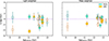 |
Fig. A.1. Differences of average weighted ages between the results of the sMILES models and those from comparison models. MILES predictions are indicated in green and WO9 results with yellow. The galaxy markers are as follows: NGC 1052 (hexagon), NGC 1351 (square), NGC 1380 (diamond), NGC 1399 (triangle), and NGC 1404 (circle). The filled and empty markers indicate the inner and outer region, respectively. |
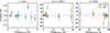 |
Fig. A.2. Differences of mass-weighted age fractions between the results of the sMILES models and those of comparison models. The marker descriptions are the same as those in Fig. A.1. |
A.2. Total metallicity
The sMILES metallicities are in a good agreement with the MILES results, as shown in Fig. A.3. However, some discrepancies are present compared to the W09 values. The W09 templates give lower metallicity in places where sMILES recover solar metallicity or higher. The exception to this is in the inner region of NGC 1351, where W09 produces a higher metallicity than sMILES. Whether this is related to the fact that sMILES give a sub-solar metallicity is unclear at this point. The discrepancies also mean that W09 produces a narrower range of total metallicity for our sample, −0.2 ≲ [M/H]≲ + 0.1, compared with the range of −0.3 ≲ [M/H]≲ + 0.2, recovered by both the MILES and sMILES libraries.
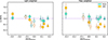 |
Fig. A.3. Differences of [M/H] between the sMILES models and those from the comparison models. The marker descriptions are the same as those in Fig. A.1. |
A.3. Alpha abundance
Overall, the sMILES templates produce higher [α/Fe] abundances than the other models. This can be seen in Fig. A.4: the sMILES values are systematically higher by ∼0.05 dex than those of MILES and ∼0.1 dex higher than the W09 results. However, since the differences are systematic, the [α/Fe] trend between the inner and outer region of each galaxy is not affected.
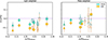 |
Fig. A.4. Differences of [α/Fe] between the sMILES models and those from the comparison models. The marker descriptions are the same as those in Fig. A.1. |
Appendix B: Distance moduli of the sample galaxies
Distance moduli for the M* analysis in Sec. 7.1.1 are presented in Table B.1. The PNLF distances are taken from Paper I for NGC 1380 and from Paper II for the rest of the sample. For NGC 1052, the SBF distance is adopted from Tonry et al. (2001), otherwise the SBF distances are adopted from Blakeslee et al. (2009). The TRGB distances are only available for NGC 1380, NGC 1399, and NGC 1404 and provided by Anand et al. (2024b).
Distance modulus for each galaxy derived using three methods: PNLF, SBF, and TRGB.
All Tables
Distance modulus for each galaxy derived using three methods: PNLF, SBF, and TRGB.
All Figures
|
Fig. 1. PN sub-sample definitions for our galaxies. The orange circles represent the positions of the inner region PNe, and the purple squares denote the positions of the outer sub-sample. The galaxy surface brightness is logarithmically scaled in the same manner for all galaxies. Following Paper II, we exclude the inner 15″ of NGC 1399 as the PNe sample in that region is incomplete. |
| In the text | |
|
Fig. 2. PNLFs of the inner and outer region of NGC 1052, binned in 0.2 mag intervals. The solid and open points represent data brighter than and fainter than the completeness limit, respectively. The curves show the analytic PNLF, shifted using the most likely apparent distance modulus and normalization. |
| In the text | |
|
Fig. 3. PNLFs of the inner and outer regions of NGC 1351, binned in 0.2 mag intervals. The solid and open points represent data brighter than and fainter than the completeness limit, respectively. One overluminous PN was excluded from the outer PN sample; that object is also shown as an open circle. The curves show the analytic PNLF, shifted using the most likely apparent distance modulus and normalization. |
| In the text | |
|
Fig. 4. PNLFs of the inner and outer region of NGC 1380, binned in 0.2 mag intervals. The solid and open points represent PN bins brighter than and fainter than the completeness limit, respectively. One overluminous PN was excluded from the outer PNLF sample, and is shown as an open circle. The curves show the analytic PNLF, shifted using the most likely apparent distance modulus and normalization. |
| In the text | |
|
Fig. 5. PNLFs of the inner and outer region of NGC 1399, binned in 0.2 mag intervals. The solid and open data points represent data brighter than and fainter than the completeness limit, respectively. The curves show the analytic PNLF, shifted using the most likely apparent distance modulus and normalization. |
| In the text | |
|
Fig. 6. PNLFs of the inner and outer region of NGC 1404, binned in 0.2 mag intervals. The solid and open data points represent data brighter than and fainter than the completeness limit, respectively. The curves show the analytic PNLF, shifted using the most likely apparent distance modulus and normalization. |
| In the text | |
|
Fig. 7. Comparison of the stellar population age (left) and total metallicity (right) between the observations and the simulations. The solid and open markers indicate the inner and outer annulus, respectively. The dashed line indicates the one-to-one comparison. |
| In the text | |
|
Fig. 8. Age and metallicity differences between the inner and outer regions of each observed galaxies (left) and the simulation analogues (right). The dot-dashed lines and the highlights indicate the weighted average and standard deviation, respectively. |
| In the text | |
|
Fig. 9. M* derived using three distance determination methods: PNLF, SBF, and TRGB. The PNLF method assumes M* = −4.54 and acts as a reference point for this comparison. The dot-dashed lines indicate the weighted average. The solid and open markers denote the inner and outer annulus, respectively. The highlights indicate the standard deviation. |
| In the text | |
|
Fig. 10. M* from our simulation analogues as a function of total metallicity (left) and age (right). The dot-dashed lines indicate the weighted average. The solid and open markers represent the inner and outer annuli, respectively. The highlights illustrate the standard deviation. We note that the x- and y-axis ranges are different to those in Fig. 9. |
| In the text | |
|
Fig. 11. Inner annulus minus outer annulus difference in M* vs. that for metallicity and age for the observations (left) and simulation analogues (right). The dot-dashed lines indicate the weighted average. The highlights show the standard deviation. |
| In the text | |
|
Fig. 12. Galaxy α0.5 values as a function of the mass fraction of young (Age < 2 Gyr), intermediate (2 ≥ Age ≥ 10 Gyr), and old (Age > 10 Gyr) stars. Upper panels: Observations. Lower panels: Values from the simulations. The green dot-dashed lines show the best-fit regressions; fits that exclude the observational data for NGC 1351 are shown as a brown dashed line. |
| In the text | |
|
Fig. 13. Left and middle: Our α0.5 measurements as a function of [M/H] for the simulations and observations, respectively. Right: Our calculated [α/Fe] values for the observations. The green dot-dashed lines show our best fit regressions; fits that exclude NGC 1351 are denoted by the dashed brown line. |
| In the text | |
|
Fig. 14. Production efficiency for PNe within 0.5 mag of M* vs. the mass fraction of stars with ages less than 10 Gyr for the five galaxies in our survey. Left: Observations data. Right: Predictions from the simulated galaxies. The arrows indicate uncertainties that reach values of less than 1%. |
| In the text | |
|
Fig. A.1. Differences of average weighted ages between the results of the sMILES models and those from comparison models. MILES predictions are indicated in green and WO9 results with yellow. The galaxy markers are as follows: NGC 1052 (hexagon), NGC 1351 (square), NGC 1380 (diamond), NGC 1399 (triangle), and NGC 1404 (circle). The filled and empty markers indicate the inner and outer region, respectively. |
| In the text | |
|
Fig. A.2. Differences of mass-weighted age fractions between the results of the sMILES models and those of comparison models. The marker descriptions are the same as those in Fig. A.1. |
| In the text | |
|
Fig. A.3. Differences of [M/H] between the sMILES models and those from the comparison models. The marker descriptions are the same as those in Fig. A.1. |
| In the text | |
|
Fig. A.4. Differences of [α/Fe] between the sMILES models and those from the comparison models. The marker descriptions are the same as those in Fig. A.1. |
| In the text | |
Current usage metrics show cumulative count of Article Views (full-text article views including HTML views, PDF and ePub downloads, according to the available data) and Abstracts Views on Vision4Press platform.
Data correspond to usage on the plateform after 2015. The current usage metrics is available 48-96 hours after online publication and is updated daily on week days.
Initial download of the metrics may take a while.