| Issue |
A&A
Volume 704, December 2025
|
|
|---|---|---|
| Article Number | L10 | |
| Number of page(s) | 4 | |
| Section | Letters to the Editor | |
| DOI | https://doi.org/10.1051/0004-6361/202557289 | |
| Published online | 05 December 2025 | |
Letter to the Editor
The TeV emission of 3C273: Inverse Compton radiation from shear-accelerated high-energy electrons in the large-scale jet?
INAF – Osservatorio Astronomico di Brera, Via E. Bianchi 46, I-23807 Merate, Italy
★ Corresponding author: This email address is being protected from spambots. You need JavaScript enabled to view it.
Received:
17
September
2025
Accepted:
6
November
2025
Abstract
The VERITAS Collaboration recently reported the detection of very high-energy (VHE) gamma-ray emission from the prototypical radio quasar 3C273. The temporal and spectral properties of this component do not appear compatible with the extrapolation of the beamed blazar-like emission of the inner, parsec-scale jet. We explore the possibility that the VHE component is produced in the jet at kiloparsec scales through the inverse Compton emission of a population of ultra-high-energy electrons (with Lorentz factor γ ∼ 108). In the model these electrons are accelerated through the shear acceleration mechanism, and they account for the still puzzling X-ray emission of knots detected by Chandra in the large-scale jets of several powerful quasars (including 3C273). In our scenario, the VHE component can be interpreted as the integrated emission from the two brightest knots of the 3C273 jet. We speculate that the decay of the emission on a timescale of ∼3 years could be accounted for by the scenario if the VHE radiation is produced in some compact regions in the downstream flow of a recollimation shock.
Key words: acceleration of particles / radiation mechanisms: non-thermal / galaxies: jets / quasars: individual: 3C 273
© The Authors 2025
 Open Access article, published by EDP Sciences, under the terms of the Creative Commons Attribution License (https://creativecommons.org/licenses/by/4.0), which permits unrestricted use, distribution, and reproduction in any medium, provided the original work is properly cited.
This article is published in open access under the Subscribe to Open model. This email address is being protected from spambots. You need JavaScript enabled to view it. to support open access publication.
1. Introduction
Despite two decades of observational and theoretical efforts, the nature of the optical and X-ray emission from compact features (knots) in large-scale jets of powerful radio-loud quasars is still debated (for a review, see Harris & Krawczynski 2006). One widely discussed model assumes that the X-ray emission is produced by relativistic electrons through inverse Compton (IC) scattering of the cosmic microwave background (CMB; Tavecchio et al. 2000; Celotti et al. 2001). This IC CMB model is strongly challenged by the good upper limits placed in the GeV band by Fermi/Large Area Telescope (LAT) (e.g., Meyer & Georganopoulos 2014; Meyer et al. 2015) and by the morphological (Tavecchio et al. 2003) and spectral (Jester et al. 2006) properties of the emission. A potential viable alternative invokes the presence of two distinct electron populations: one at low energies (LEs), responsible for the emission from radio to the optical band, and an ultra-high-energy population (with Lorentz factors γ ∼ 107 − 8) emitting X-rays through synchrotron radiation in magnetic fields (B) of ∼10 μG (e.g., Harris & Krawczynski 2002; Kataoka & Stawarz 2005). This scenario would also explain the high degree of polarization (> 30%) measured in the optical band for a component in the jet of the quasar PKS 1136-135, whose optical emission belongs to the high-energy (HE) emission component (Cara et al. 2013).
A specific model based on the double-population scenario is presented in Tavecchio (2021). The model assumes that LE electrons are accelerated at shocks through the standard diffusive shock acceleration mechanism, while electrons further energized through shear acceleration (Rieger 2019; Rieger & Duffy 2022; Wang et al. 2023) form a narrow distribution, producing synchrotron X-ray emission. The model is able to explain the observed spectral energy distribution (SED) of the knots, with an acceptable energy budget for the jets. In the Tavecchio (2021) model, the jet is only mildly relativistic, with bulk Lorentz factors (Γ) of ∼2, thus avoiding the overproduction of GeV gamma rays through the IC CMB mechanism as constrained by Fermi/LAT. However, both the LE and HE electron populations produce high and very high gamma-ray radiation through the IC scattering of synchrotron photons and the CMB. The resulting non-negligible gamma-ray emission extends into the TeV band.
The Very Energetic Radiation Imaging Telescope Array System (VERITAS) collaboration has recently reported the detection of very high-energy (VHE) emission from the prototypical radio-quasar 3C 2731. The light curve shows evidence of a possible variation (i.e., decay) of the flux with a timescale of ∼3 years. The (time-integrated) hard spectrum, which has a positive slope in the νF(ν) representation, is incompatible with the extrapolation of the soft tail of the blazar γ-ray component recorded in the GeV band by Fermi/LAT that is associated with the IC emission from the inner, parsec-scale jet (e.g., Ghisellini et al. 2010). A feasible explanation would be the presence of an additional emission component associated with the blazar region (possibly of hadronic origin). In this paper we instead explore the possibility that the VHE component flags the expected integrated IC emission produced by the HE, shear-accelerated electrons in the large-scale (kiloparsec-scale) jet.
The paper is organized as follows. In Sect. 2 we present a sketch of the model, in Sect. 3 we discuss the results, and we conclude in Sect. 4. Throughout the paper, the following cosmological parameters are assumed: H0 = 70 km s−1 Mpc−1, ΩM = 0.3, and ΩΛ = 0.7.
2. The model
We sketch below the main elements of the model. For a detailed description, the reader is referred to Tavecchio (2021).
As mentioned above, we assumed that the LE (radio to optical) emission of knots in 3C273 is produced by relativistic electrons accelerated by a shock (“LE electrons” in the following). We assumed that these electrons follow a cutoff power-law energy distribution with slope nsh:
 (1)
(1)
where K is a normalization and γcut is the maximum Lorentz factor reached by the particles.
The jet is characterized by a velocity structure, with a core of constant speed surrounded by a shear layer in which the plasma speed, βj(r), decreases along the radial direction, r. The shear could be the result of the interaction of the jet with the external material and the triggering of the Kelvin-Helmholtz instability (e.g., Borse et al. 2021; Wang et al. 2023). We used the following simple linear parametrization for the velocity profile:
 (2)
(2)
where rj is the jet radius and ΔL characterizes the thickness of the layer. The precise shape of the profile can affect the resulting electron energy distribution (e.g., Rieger & Duffy 2022). However, considering the limited quality of the data, the particular choice is not expected to have a major impact on the model. A small fraction of the LE electrons accelerated at the shock enter the sheath in the downstream region, where they experience further energization through scattering with magnetic turbulence (the “HE electron component” in the following).
To model the shear acceleration process, we followed Liu et al. (2017), who used an approximate Fokker-Planck treatment to model the time-dependent evolution of the electron energy distribution. A key parameter regulating the shear acceleration process is the mean free path of particles scattered by magnetic turbulence, λ, which can be written as
 (3)
(3)
where γ is the particle Lorentz factor, rg is the particle gyration radius, ξ = δB2/B2 is the ratio between the energy density of the turbulent and regular magnetic fields, Λ is the maximum wavelength of turbulence interacting with the particles, and q is the slope of the power-law spectrum of the turbulent field in the wavenumber space. In the following we fix q = 5/3, which corresponds to the Kolmogorov spectrum.
A second important parameter regulating the acceleration efficiency is related to the velocity profile and is defined as A = Γj(r)2|∂rβj(r)|c, where Γj(r) = [1 − βj(r)2]−1/2 is the flow bulk Lorentz factor. The acceleration timescale can be written as
 (4)
(4)
Note that tacc ∝ (γ/B)−1/3 for q = 5/3, and therefore tacc decreases with the particle energy, i.e., particles with high Lorentz factor are more efficiently accelerated than those with small Lorentz factor. This is the reason why a population of pre-accelerated electrons is required for this mechanism to work efficiently. On the other hand, large magnetic fields, which determine small electron gyroradii and thus small λ, imply long acceleration times.
Particles can also diffusively escape from the acceleration layer. We approximated the escape time considering the diffusion of particles from a region with a size comparable to the shear layer thickness (ΔL), i.e., tesc(γ)≃ΔL2/2κ. Here one can use the standard expression κ = cλ/3 for the spatial diffusion coefficient. To ensure acceleration, we have to assume tacc < tesc.
At VHEs, the mean free path of the electrons becomes comparable to the size of the jet layer, ΔL. Beyond this point, the particles escape from the system and cannot be further accelerated. This fixes a geometrical maximum limit (γg, max) for the accelerating electrons: λ(γg, max) = ΔL.
Both LE and HE electrons emit electromagnetic radiation through synchrotron and IC mechanisms. For the latter, we considered both photons locally produced in the jet and CMB photons. The radiative losses determine a second (radiative) limit to the maximum energy reached by the electrons, γr, max, set by the balance between cooling and acceleration timescales. The radiative cooling time is
 (5)
(5)
where UB is the magnetic field energy density, and the total radiation energy density includes the contribution of LE synchrotron photons emitted by electrons in the downstream region and the CMB photons, Urad = Usyn + UCMB (we neglected the IC emission off the synchrotron photons produced by HE electrons because scatterings occur deep into the Klein-Nishina regime). As we will see, in the case considered here, the limiting energy set by the radiative losses is much higher than that determined by the mean free path. The maximum energy of the electrons is thus determined by the geometrical limit, γg, max.
The treatment used here adopts a leaky-box, spatially averaged approximation of the shear acceleration process (Rieger & Duffy 2022) that leads to a Fokker-Planck equation prescribing the evolution of the electron energy distribution (Liu et al. 2017). As in the case of the velocity profile, the details of the spatial transport are not expected to be highly relevant in the present context. Numerically, we solved the equation by using the robust implicit method of Chang & Cooper (1970). We assumed that a fraction of the particles downstream of the shock, characterized by the distribution n0(γ) defined by Eq. (1), enters the shear acceleration process. The injection rate can be phenomenologically described by an injection time, τinj, related to the diffusion time in the downstream region. For simplicity, we assumed an energy-independent timescale. Therefore, we assumed a constant injection with spectrum Q(γ) = n0(γ)/τinj. As shown in Tavecchio (2021), to reproduce the hard optical-X ray continuum traced by the data, the source needs to survive long enough to reach an equilibrium state. For shorter lifetimes, the incompletely developed bump displays a relatively soft spectrum that is incompatible with the optical and X-ray fluxes. Therefore, we calculated the HE component until an approximate equilibrium state was reached.
For the application to 3C273, we fixed some parameters to benchmark values. In particular, we assumed B = 10 μG (both in the core and in the sheath) and Γj(0) = 2 for both knots A and B. We assumed a viewing angle of 15 degrees, which implies a Doppler factor (relevant for the boosting of the emission) of 3. For definiteness, we also fixed ΔL = 0.2rj, ξ = 0.1, and Λ = ΔL. The assumption that the observed decay timescale of the VHE emission, t ∼ 3 years, is dictated by the light-crossing time of the emitting region (see the discussion below), together with the assumed δ, implies a dimension of the source (which in our scenario should be identified with the shear layer) of ≈109 cm.
3. Results
Tuning the free parameters, we first reproduced with the LE component the radio-to-optical SED of the two brightest knots, called knots A and B in Sambruna et al. (2001). We matched the second emission component, produced by HE electrons accelerated within the velocity shear, to the X-ray data by regulating the only remaining free parameter, the injection timescale, τinj, for which we derive ∼102 yrs in both cases.
We show the data points (radio, optical, and X-rays) in Fig. 1, together with the results of the modeling (whose parameters are reported in Table 1). In the plot we show all radiative components from both the LE and HE electron populations. In particular, the synchrotron radiation of the LE electrons accounts for the radio-to-optical components, while the HE population produces the X-ray emission. IC components from both LEs and HEs contribute to the emission in the gamma-ray band. Note that the IC scattering of HE electrons with the synchrotron photons produced by themselves is deeply into the Klein-Nishina regime and is therefore strongly suppressed. HE electrons therefore emit IC radiation mainly through the scattering of the CMB and the synchrotron photons emitted by LE electrons. As is visible in Fig. 1, the main contribution to the emission in the TeV band comes from the latter component. We remark that the X-ray emission corresponds, for both knots, to the peak of the HE synchrotron component. This agrees with the results of Jester et al. (2006), who noted that the X-ray emission of knots in 3C273 is softer than the corresponding radio spectrum.
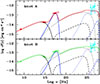 |
Fig. 1. SED (circles) of knots A (upper panel) and B (lower panel) of the jet of 3C273 (from Sambruna et al. 2001; we also report the X-ray spectral slopes derived in He et al. 2023). Light blue data points report the (EBL-deabsorbed) VERITAS spectrum. The lines show the result of the model for the electrons accelerated at the shock (black) and at the shear (blue); solid lines for synchrotron, dotted lines for IC from synchrotron, and dashed lines for the IC CMB model. The red and green lines report the total emission. |
Parameters of the model.
In Fig. 2 we show the SED of the 3C273 core (gray data points), together with the VERITAS data points. The black curves show the integrated emission from knots A and B, which accounts for the observed VHE component. For the model we used rj < 1020 cm so that the width of the shear layer, ΔL = 0.2rj (which in our model quantifies the size of the emission region of HE electrons and hence determines the variability timescale of the VHE component), is close to the constraint posed by variability (≈1019 cm when beaming is taken into account).
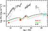 |
Fig. 2. Historical SED data for the 3C273 core (gray) with the VERITAS spectrum (light blue) and the SED of knots A and B. Red, green, and black lines show the emission from knot A, knot B, and the total, respectively. |
In Fig. 3 we show the timescales of the different processes as a function of the electron Lorentz factor for knot A. It is clear that the radiative cooling time (dominated by the IC losses; dotted blue line) greatly exceeds the acceleration timescale at all energies. Therefore, radiative losses do not limit the acceleration. Instead, the maximum energy of the shear-accelerated electrons is set by the geometrical limit (dashed vertical line) at γg, max ≃ 108.
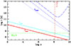 |
Fig. 3. Timescales (in the source frame) relevant for the shear acceleration process as a function of the particle Lorentz factor for knot A. Solid lines show the acceleration (red) and escape (light blue) timescales. The darker blue curves show the cooling times for the synchrotron (dashed), IC on the synchrotron photons (dotted), and the IC CMB model (long-dashed). The vertical dashed orange line shows the Lorentz factor above which the mean free path exceeds the width of the shear layer, halting the acceleration process. The horizontal dashed green line indicates the light-crossing time of the shear layer. |
With the physical parameters derived from our models, the inferred power carried by the jet (including one cold proton per relativistic electron) is PJ = 3 × 1046 erg s−1. This is lower than the power derived for the inner jet from the modeling of the SED of the core (e.g., Ghisellini et al. 2010).
4. Discussion
We have shown that a scenario based on two populations of relativistic electrons (Tavecchio 2021) can satisfactorily reproduce the multifrequency emission of the two brightest knots of the kiloparsec-scale jet of 3C273 and can naturally account for the hard VHE spectrum measured by VERITAS, interpreted as the integrated IC emission of the knots. The specific scenario that we adopted assumes that the two electron populations are produced through the joint action of diffusive shock acceleration and shear-acceleration mechanisms. A model based on shear acceleration has already been applied to interpret the emission of large-scale jets in radio-loud quasars and radio galaxies (Tavecchio 2021; He et al. 2023; Wang et al. 2023). He et al. (2023) and Wang et al. (2023) also considered the emission from 3C273, but their models predict a flux in the TeV band well below that detected by VERITAS.
The model’s most challenging constraint comes from the decay timescale of the recorded VHE flux, which is on the order of about 3 years, i.e., tdec ∼ 108 s. This directly limits the (Doppler-corrected) size (R) of the emitting region to ≲1019 cm. In the scheme, the region responsible for the VHE radiation is identified with the shear, with a size of ΔL = 0.2rj, and thus poses an upper limit of rj ≲ 1020 cm for the jet radius.
Furthermore, to account for the observed decay, we had to assume that particles emitting gamma rays at VHEs, with γ ∼ 108, must either cool or escape from the source in less than ≃3 × 10⁸ s. Although radiative cooling is quite inefficient, Fig. 3 shows that particles can cool through adiabatic losses (on the order of the light-crossing time, ΔL/c) or diffuse out of the shear layer in a comparable time.
We note that the compact dimensions of the source, a constraint primarily determined by the decay timescale of the observed flux, naturally ensures a high output through the IC component(s), an ingredient that is key to reaching the relatively high flux required by the VERITAS data. We also remark that in our scenario the variability of the VHE emission should be reflected in the X-ray band since HE electrons are responsible for the emission in both bands. To our knowledge, there are no Chandra observations of 3C273 in the period corresponding to the VHE flux decay. Therefore, it is not possible to directly test this prediction. However, variability in the X-ray knot emission on 1-year timescales has been detected in other jets, most notably Pictor A (Marshall et al. 2010).
The small size of the emission regions flagged by the short-term variability clearly represents a challenge for our understanding of the emission from large-scale jets (see also Marshall et al. 2010). In the specific case of 3C273, knots A and B, the sites of the VHE emission, lie at distances on the order of 1023 cm from the central black hole (de-projected with an assumed viewing angle of 15 deg). Assuming a simple conical geometry for the jet, this would imply an implausibly small jet opening angle (θj) of ∼10−3 (at very long baseline interferometry scales, observations suggest Γjθj = 0.2, which in our case would imply θj = 0.1; Pushkarev et al. 2009). As a possible way out of this conundrum, we advance the hypothesis that knots mark the position of strong recollimation shocks (e.g., Komissarov & Falle 1997). These structures form when the imbalance between the jet and the external pressures forces the jet streamlines to bend toward the jet axis, forming an oblique shock followed by a reflection shock. In the complex region downstream of the recollimation shock (where the jet reaches its minimum radius and the reflection shock starts), particles can be accelerated and emit radiation (e.g., Sciaccaluga et al. 2025). Magnetohydrodynamic simulations (e.g., Matsumoto et al. 2021; Costa et al. 2024) show that most of the dissipation (and hence emission) occurs after the reflection shock in very compact regions, potentially much smaller than the jet radius (Bodo & Tavecchio 2018). Moreover, the flow in these regions develops a complex structure, with steep velocity gradients that can potentially provide the ideal conditions for efficient shear acceleration. Dedicated simulations beyond the scope of this paper, that include details of the acceleration processes, should be performed to assess this scenario.
The upcoming Cherenkov Telescope Array, with its improved sensitivity, will be able to easily confirm the VERITAS detection and provide high-quality data that can be compared with models. Particularly interesting will be the investigation of the temporal behavior of the emission that, as discussed above, provides strong constraints for models. Of the known powerful, large-scale quasar jets with bright knots, 3C 273 is one of the closest to Earth (z = 0.158). This, besides implying a large high flux, means that a relatively small amount of the VHE radiation is absorbed through the pair production process with the Extragalactiv Background Light (Franceschini & Rodighiero 2017). Sources located at greater distances (e.g., the prototypical source PKS 0637-752 at z = 0.651) are likely characterized by a lower flux and greater EBL suppression. Although dedicated simulations of the observational feasibility are required, one can tentatively conclude that detection of VHE emission from other large-scale jets hosted by powerful quasars is probably very challenging.
A presentation can be found at https://indico.cern.ch/event/1258933/contributions/6491204/attachments/3104111/5500883/Benbow_ICRC2025.tif
Acknowledgments
I thank the referee for useful comments. I would like to thank S. Boula and P. Coppi for useful and encouraging discussions. FT acknowledges financial support from INAF Theory Grant 2024 (PI F. Tavecchio) This work has been funded by the European Union-Next Generation EU, PRIN 2022 RFF M4C21.1 (2022C9TNNX). Part of this work is based on archival data provided by the ASI-SSDC.
References
- Bodo, G., & Tavecchio, F. 2018, A&A, 609, A122 [NASA ADS] [CrossRef] [EDP Sciences] [Google Scholar]
- Borse, N., Acharya, S., Vaidya, B., et al. 2021, A&A, 649, A150 [NASA ADS] [CrossRef] [EDP Sciences] [Google Scholar]
- Cara, M., Perlman, E. S., Uchiyama, Y., et al. 2013, ApJ, 773, 186 [CrossRef] [Google Scholar]
- Celotti, A., Ghisellini, G., & Chiaberge, M. 2001, MNRAS, 321, L1 [Google Scholar]
- Chang, J. S., & Cooper, G. 1970, J. Comput. Phys., 6, 1 [Google Scholar]
- Costa, A., Bodo, G., Tavecchio, F., et al. 2024, A&A, 682, L19 [NASA ADS] [CrossRef] [EDP Sciences] [Google Scholar]
- Franceschini, A., & Rodighiero, G. 2017, A&A, 603, A34 [NASA ADS] [CrossRef] [EDP Sciences] [Google Scholar]
- Ghisellini, G., Tavecchio, F., Foschini, L., et al. 2010, MNRAS, 402, 497 [Google Scholar]
- Harris, D. E., & Krawczynski, H. 2002, ApJ, 565, 244 [NASA ADS] [CrossRef] [Google Scholar]
- Harris, D. E., & Krawczynski, H. 2006, ARA&A, 44, 463 [NASA ADS] [CrossRef] [Google Scholar]
- He, J.-C., Sun, X.-N., Wang, J.-S., et al. 2023, MNRAS, 525, 5298 [Google Scholar]
- Jester, S., Harris, D. E., Marshall, H. L., & Meisenheimer, K. 2006, ApJ, 648, 900 [Google Scholar]
- Kataoka, J., & Stawarz, Ł. 2005, ApJ, 622, 797 [NASA ADS] [CrossRef] [Google Scholar]
- Komissarov, S. S., & Falle, S. A. E. G. 1997, MNRAS, 288, 833 [Google Scholar]
- Liu, R.-Y., Rieger, F. M., & Aharonian, F. A. 2017, ApJ, 842, 39 [NASA ADS] [CrossRef] [Google Scholar]
- Marshall, H. L., Hardcastle, M. J., Birkinshaw, M., et al. 2010, ApJ, 714, L213 [NASA ADS] [CrossRef] [Google Scholar]
- Matsumoto, J., Komissarov, S. S., & Gourgouliatos, K. N. 2021, MNRAS, 503, 4918 [NASA ADS] [CrossRef] [Google Scholar]
- Meyer, E. T., & Georganopoulos, M. 2014, ApJ, 780, L27 [Google Scholar]
- Meyer, E. T., Georganopoulos, M., Sparks, W. B., et al. 2015, ApJ, 805, 154 [NASA ADS] [CrossRef] [Google Scholar]
- Pushkarev, A. B., Kovalev, Y. Y., Lister, M. L., & Savolainen, T. 2009, A&A, 507, L33 [NASA ADS] [CrossRef] [EDP Sciences] [Google Scholar]
- Rieger, F. M. 2019, Galaxies, 7, 78 [NASA ADS] [CrossRef] [Google Scholar]
- Rieger, F. M., & Duffy, P. 2022, ApJ, 933, 149 [Google Scholar]
- Sambruna, R. M., Urry, C. M., Tavecchio, F., et al. 2001, ApJ, 549, L161 [NASA ADS] [CrossRef] [Google Scholar]
- Sciaccaluga, A., Costa, A., Tavecchio, F., et al. 2025, A&A, 699, A296 [NASA ADS] [CrossRef] [EDP Sciences] [Google Scholar]
- Tavecchio, F. 2021, MNRAS, 501, 6199 [Google Scholar]
- Tavecchio, F., Maraschi, L., Sambruna, R. M., & Urry, C. M. 2000, ApJ, 544, L23 [Google Scholar]
- Tavecchio, F., Ghisellini, G., & Celotti, A. 2003, A&A, 403, 83 [NASA ADS] [CrossRef] [EDP Sciences] [Google Scholar]
- Wang, J.-S., Reville, B., Mizuno, Y., Rieger, F. M., & Aharonian, F. A. 2023, MNRAS, 519, 1872 [Google Scholar]
All Tables
All Figures
|
Fig. 1. SED (circles) of knots A (upper panel) and B (lower panel) of the jet of 3C273 (from Sambruna et al. 2001; we also report the X-ray spectral slopes derived in He et al. 2023). Light blue data points report the (EBL-deabsorbed) VERITAS spectrum. The lines show the result of the model for the electrons accelerated at the shock (black) and at the shear (blue); solid lines for synchrotron, dotted lines for IC from synchrotron, and dashed lines for the IC CMB model. The red and green lines report the total emission. |
| In the text | |
|
Fig. 2. Historical SED data for the 3C273 core (gray) with the VERITAS spectrum (light blue) and the SED of knots A and B. Red, green, and black lines show the emission from knot A, knot B, and the total, respectively. |
| In the text | |
|
Fig. 3. Timescales (in the source frame) relevant for the shear acceleration process as a function of the particle Lorentz factor for knot A. Solid lines show the acceleration (red) and escape (light blue) timescales. The darker blue curves show the cooling times for the synchrotron (dashed), IC on the synchrotron photons (dotted), and the IC CMB model (long-dashed). The vertical dashed orange line shows the Lorentz factor above which the mean free path exceeds the width of the shear layer, halting the acceleration process. The horizontal dashed green line indicates the light-crossing time of the shear layer. |
| In the text | |
Current usage metrics show cumulative count of Article Views (full-text article views including HTML views, PDF and ePub downloads, according to the available data) and Abstracts Views on Vision4Press platform.
Data correspond to usage on the plateform after 2015. The current usage metrics is available 48-96 hours after online publication and is updated daily on week days.
Initial download of the metrics may take a while.