| Issue |
A&A
Volume 705, January 2026
|
|
|---|---|---|
| Article Number | A10 | |
| Number of page(s) | 7 | |
| Section | The Sun and the Heliosphere | |
| DOI | https://doi.org/10.1051/0004-6361/202142199 | |
| Published online | 23 December 2025 | |
An unusual velocity field in a sunspot penumbra
1
Leibniz-Institut für Astrophysik Potsdam (AIP), An der Sternwarte 16, D-14482 Potsdam, Germany
2
Institut für Physik und Astronomie, Universität Potsdam, D-14476 Potsdam, Germany
3
Institut für Sonnenphysik (KIS), George-Köhler-Allee 401a, D-79110 Freiburg, Germany
4
Instituto de Astrofísica de Canarias, Vía Láctea s/n, 38205 La Laguna, Tenerife, Spain
5
Departamento de Astrofísica, Universidad de La Laguna, 38205 La Laguna, Tenerife, Spain
6
Hansa-Gymnasium, Fährwall 19, D-18439 Stralsund, Germany
7
Udaipur Solar Observatory, Physical Research Laboratory, Udaipur, India
8
Astronomical Institute of the Czech Academy of Sciences, Fričova 298, 25165 Ondřejov, Czech Republic
★ Corresponding author: This email address is being protected from spambots. You need JavaScript enabled to view it.
Received:
10
September
2021
Accepted:
30
October
2025
Abstract
Context. The photospheric Evershed flow is normally oriented radially outward, yet sometimes opposite velocities are observed not only in the chromosphere but also in the photospheric layers of the penumbra.
Aims. We studied the velocity field in a special case of an active region with two mature sunspots, the lesser of which formed several days after the main one. Flux emergence between the two spots is still ongoing, influencing the velocity pattern.
Methods. We observed the active region NOAA 12146 on August 24, 2014, with the GREGOR Fabry-Pérot Interferometer and the Blue Imaging Channel of the GREGOR solar telescope at Observatorio del Teide on Tenerife. Context data from the Helioseismic and Magnetic Imager on board the Solar Dynamics Observatory complement the high-resolution data.
Results. In the penumbra of a newly formed spot, we observe opposite Doppler velocity streams of up to ±2 km s−1 very close to each other. These velocities extend beyond the outer penumbral boundary and cross the polarity-inversion line. The properties of the magnetic field do not change significantly between these two streams. Although the magnetic field is almost horizontal, we do not detect high transversal velocities in horizontal flow maps obtained via the local correlation technique.
Conclusions. The ongoing emergence of magnetic flux in an active region causes flows of opposite directions that penetrate the penumbra of a preexisting sunspot.
Key words: techniques: spectroscopic / Sun: magnetic fields / sunspots
© The Authors 2025
 Open Access article, published by EDP Sciences, under the terms of the Creative Commons Attribution License (https://creativecommons.org/licenses/by/4.0), which permits unrestricted use, distribution, and reproduction in any medium, provided the original work is properly cited.
This article is published in open access under the Subscribe to Open model. This email address is being protected from spambots. You need JavaScript enabled to view it. to support open access publication.
1. Introduction
Regular sunspots exhibit the Evershed flow (EF) in their penumbra. It is an outward flow with a velocity of about 2 km s−1 (see Solanki 2003). The line profiles in the penumbra are asymmetric, providing a hint that the EF is height-dependent. Stellmacher & Wiehr (1980) studied different spectral lines and found decreasing velocities with height in the solar atmosphere. Balthasar et al. (1997) investigated three spectral lines formed in different atmospheric layers. The lines were recorded simultaneously, and shifts due to the Earth’s motion were corrected. In deep layers, they found velocities of up to 3 km s−1, in medium heights about 1 km s−1, and in high photospheric layers velocities close to zero on an absolute wavelength scale. Wiehr (1995) investigated the asymmetries and explained them as a superposition of two different velocities. The faster component can be more than 5 km s−1. In chromospheric and higher layers, an inverse EF is observed (St. John 1913). In contrast to the photosphere, flow velocities in the chromosphere increase with height. Alissandrakis et al. (1988) reported peak velocities of −1.7 km s−1 in the photosphere, +1.7 km s−1 in the low chromosphere, 2.5 km s−1 in the higher chromosphere, and 15 km s−1 in the transition region. In a recent investigation, Choudhary & Beck (2018) found partly supersonic velocities from the chromospheric spectral line Ca II 854.2 nm, in contrast to Tsiropoula (2000), who found subsonic velocities from Hα. The inverse EF is explained as a siphon flow by Choudhary & Beck (2018), but for the photospheric EF, an overturning convection causes the magnetized outflow (see Rempel 2015).
Anomalous flows in the photosphere of sunspot penumbrae were observed in several cases. Louis et al. (2011) observed three sunspots with locations where Doppler shifts opposite to the normal EF were detected. Close to the umbra–penumbra boundary, they are interpreted as supersonic downflows. Kleint & Sainz Dalda (2013) investigated a sunspot with bright filaments penetrating unusually far into the umbra. A feature on the limb side shows blueshifts in the penumbra and redshifts inside the umbra, and the opposite behavior was found on the center side. Louis et al. (2014) observed a blueshifted feature embedded in the limb-side penumbra with a velocity of 1.6 km s−1. The magnetic field in this feature was almost horizontal, and the feature occurred in the prolongation of a light bridge. It was accompanied by a redshifted area next to it. Louis et al. (2020) investigated an atypical light bridge that produces a blueshift that reaches into the limb-side penumbra, where the normal EF exhibits a redshift. Another case of blueshifts in the limb-side penumbra, related to an umbral filament, was investigated by Guglielmino et al. (2019). Balthasar et al. (2016) found redshifts in a center-side penumbra when there was an arch filament system (AFS) between the spot and the neighboring pores. Some footpoints of the AFS were located in the penumbra. An AFS occur when new flux is emerging and matter is streaming downward along the magnetic field lines in the arch filaments. Siu-Tapia et al. (2017) report a case where in a part of the penumbra the flow was inward, i.e., reversed with respect to the regular EF, and called it a counter-EF. They used data recorded with the Hinode Solar Optical Telescope and its spectropolarimeter in the spectral lines Fe I 630.15 nm and Fe I 630.25 nm, which form in mid-photospheric layers. The magnetic field is more horizontal at the location of the counter-EF than in the areas with normal EF. With numerical simulations, Siu-Tapia et al. (2018) interpreted the normal EF originating from overturning convection, finding that, on a few occasions, a counter-EF caused by a siphon flow occurred for limited time intervals. Murabito et al. (2018) studied 12 active regions with 17 spots (10 preceding, 7 following) during the formation of a penumbra. In 11 cases, they found counter-EFs before the penumbrae became detectable. A more detailed statistical analysis on how often counter-EFs appear is presented by Castellanos Durán et al. (2021). They find that 81 out of the 97 active regions they analyzed show counter-EFs, and they find a median of six cases of counter-EFs per active region. Many cases are related to light bridges or deviations of the vertical magnetic field from the surroundings. Flows opposite to the normal EF also are observed before a penumbra is formed or restored (see Romano et al. 2020 and García-Rivas et al. 2024).
We investigated an active region with newly emerging magnetic flux next to a preexisting sunspot and studied in particular the velocity field related to the new flux. We focused on an unusual velocity field in this sunspot group.
2. Observations
We observed active region NOAA 12146 with the GREGOR solar telescope (Schmidt et al. 2012) and the GREGOR Fabry-Pérot Interferometer (GFPI; Denker et al. 2010; Puschmann et al. 2012) in spectroscopic mode from 09:43 until 09:59 UT on August 24, 2014. The region was located at 10° north and 20° west. An overview of the active region is provided in Fig. 1. We selected the spectral line Fe I 709 nm, which does not split in the magnetic field. This line has an excitation potential of 4.23 eV and probes medium heights in the photosphere. We recorded 24 positions along the line profile with a single exposure time of 45 ms and accumulated eight images per wavelength step. A scan through the line profile took about 31 s. The step width in wavelength was 2.363 pm, and the pixel size of the GFPI camera corresponds to 0 079. To get the wavelength of 709 nm to the GFPI, we had to replace the standard pentaprism dividing the light between GFPI and the GREGOR Infrared Spectrograph (GRIS; Collados et al. 2012) with a three-mirror system1 and thus we could not use GRIS in parallel. After correction for dark currents and flat fields, the images were reconstructed via multi-object multi-frame blind deconvolution (Löfdahl et al. 2002; van Noort et al. 2005) using eight images per wavelength step. The images from the continuum channel, which were taken strictly simultaneously, were used to align the images along the spectral scan after determining the instrumental alignment using pinhole and target recordings. In the next step, the instrumental blueshift of the GFPI was corrected in the data. Then we removed the transmission curve of the prefilter. Finally, we corrected the internal image rotation of the GREGOR telescope within the series of 30 scans through the line profile. The de-rotator was installed only after our observations. These reduction routines are available in the sTools data processing pipeline (Kuckein et al. 2017).
 |
Fig. 1. White-light image of the active region obtained with HMI at 09:48 UT on August 24, 2014. The red box marks the field of view of GFPI. The black arrow points to the solar disk center. |
Velocities were determined in two different ways, either by a fourth-order polynomial fit or by the Fourier method described in Schlichenmaier & Schmidt (2000). The results are somewhat different. The polynomial fit yields the position of the line core (minimum), while the Fourier method represents the position of the line as a whole. Differences between the methods are due to line asymmetries and because of the line core forming in higher layers of the photosphere than the rest of the line. Nevertheless, the global view is quite similar. The zero-point reference is the mean value in a vertical stripe on the right side of the GFPI part in Fig. 1, which represents the average of granular and intergranular velocities. We note that this reference is not necessarily an absolute one.
Context images were obtained at GREGOR with two pco4000 CCD cameras mounted on the Blue Imaging Channel (BIC; Puschmann et al. 2012), first mentioned in Denker et al. (2010), using a G-band filter (430 nm) and a blue continuum filter (450 nm). We took repetitive bursts of 100 images with an exposure time of 5 ms in the G band and 4 ms in the blue continuum. The series of bursts were started when the GFPI recording was started and stopped when the GFPI recording finished. We obtained 32 bursts in the G band and 28 in the blue continuum. The two cameras were controlled by two different computers. The images were corrected for dark currents and flat fields, and each burst was processed with the Kiepenheuer-Institute Speckle Interferometry Package (KISIP; Wöger et al. 2008; Wöger & von der Lühe 2008). Thus, each burst results in a reconstructed image. An example of a blue continuum image is shown in Fig. 4a. We selected the blue continuum images because they exhibit a higher granular contrast compared to the G-band images.
To get information about the magnetic field, we downloaded data obtained with the Helioseismic and Magnetic Imager (HMI; Schou et al. 2012) on board the Solar Dynamics Observatory (SDO; Pesnell et al. 2012). We used the magnetic vector field, the Doppler velocity, and the continuum intensity. The HMI team derived the magnetic field vector using their vector magnetic field pipeline (Hoeksema et al. 2014) and by applying a very fast inversion of the Stokes vector (Borrero et al. 2011; Centeno et al. 2014). The pipeline includes the minimum energy method to solve the magnetic 180° ambiguity. We selected the data taken at 09:48 UT, which are the only ones in the 720 s series obtained during the observation period at GFPI. For the alignment, we compared the continuum images from GFPI and HMI, and cut out the common range from the HMI image (red box in Fig. 1). Then we interpolated the HMI image to the same pixel size as the GFPI image. The intensity contour lines of the two images agree, on average, to better than a distance of 0 3 on the Sun. Note that the original HMI pixel size is 0
 5.
5.
3. Results
This active region developed very quickly. On August 21, it consisted of a single regular spot of negative polarity. In the following, we describe the development of the intensity, Doppler velocity, magnetic field strength, and inclination observed by HMI between 00:00 UT on August 23 and 23:48 UT on August 24. Figure 2 shows an example of the HMI images, and an animation is available online. At 00:00 UT on August 23, a few hours after the meridian passage, a single pore of positive polarity was visible south of the main spot. Then more positive flux in the form of pores emerged. Negative flux separated from the main spot and moved toward the positive region, where it was canceled, perhaps by submerging flux loops. Finally, the positive pores merged and formed the second sunspot. On August 24, the two penumbrae came into contact but later separated again. High Doppler velocities appeared for certain periods in the area between the major spots and disappeared again. East of the two major spots was another small spot with an irregular penumbra, and several pores appeared between the main and the small spot. Most of these pores moved toward the main spot and merged with it. Next to the two major spots, the emergence of magnetic flux was still ongoing on August 25. The configuration of the vertical magnetic field is shown in Fig. 3. From this vertical component of the magnetic field, we derived the Polarity-Inversion line (PIL). Between August 22 and 29, the group caused 17 C-class flares, and on August 25 two M-class flares. On August 24, three C-class flares occurred, at 00:08, 07:26, and 11:50 UT.
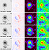 |
Fig. 2. HMI data at four time steps. Each step is displayed in a row. The columns, from left to right, show the intensity, HMI velocities, total magnetic field strength, and magnetic inclination. Velocities are scaled in the range ±2.5 km s−1, the magnetic field strength is clipped at 3000 G, and the range of inclination is 0–180°. The bar in the upper-right corner of the intensity images indicates a length of 10 Mm. An animation of this figure from 00:00 UT on August 23 until 23:48 UT on August 24 is available online. |
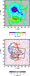 |
Fig. 3. Upper: Vertical component of the magnetic field recorded by HMI at 09:48 UT on August 24. Black and white contours indicate the boundaries of the umbra and penumbra according to Fig. 1. Values are suppressed where the total magnetic field strength is below 150 G. Lower: Corresponding Doppler velocity from HMI. |
The most prominent result of our observations is the velocity field in the penumbra of the newly formed sunspot. The 30 scans through the line profile give very similar results, which means that the feature was persistent for at least 16 minutes. Thus, we display only maps from the scan that started at 09:48:15 UT, when we had nearly simultaneous data from HMI. Velocities of up to 2 km s−1 in opposite directions appeared very close to each other, as shown in Figs. 4c and d. Some blueshifts are more prominent in the Fourier method results (Fig. 4d), probably because the Fourier method is more sensitive to the whole line profile stemming from deeper layers than the line core, which is relevant for the polynomial fits. The flows in both directions cross the PIL, i.e., they are not separated by the PIL. At this position on the disk, we expected a velocity away from us according to the EF for the newly emerging sunspot, while very low velocities were expected for the nearby penumbra of the main spot. However, we observed blueshifts in this area, and the space between the two spots was dominated by blueshifts. These features are also seen in the HMI Doppler velocity images, but at a lower resolution.
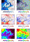 |
Fig. 4. (a): Speckle-restored blue continuum image of the investigated region obtained at GREGOR, restricted to the area recorded with the GFPI. The red contours mark the zero-velocity lines, and the yellow line the PIL. Black contours outline the outer penumbral boundary, and white the umbral–penumbral boundary. The arrow points to disk center (note the image is rotated compared to Fig. 1). (b): Horizontal velocity map obtained via the LCT. The color and length of the arrows indicate the velocity on a spectral scale (see the color bar). The average blue continuum image serves as the background. (c) and (d): Velocity maps, derived from polynomial fits (c) and from the Fourier method (d), applied to GFPI data. Red and black contours mark the umbra and penumbra according to the GFPI intensity map. The yellow line indicates the PIL. Here, trajectories of the high velocities shown in Fig. 5 are marked in light blue. (e): Total magnetic field strength. (f): Inclination of the magnetic field in the local frame of reference, taken from HMI. Black and white contours indicate the boundaries of the umbra and penumbra in the GFPI data. Values are set to 90° where the total magnetic field strength is below 150 G. The violet line marks the PIL. The trajectories are marked in panel f in black. An animation of panels c and d is available online.
|
Normally, penumbral filaments are oriented radially, but as can be seen in Fig. 4a, they deviate significantly from the radial direction, and the outer ends point more toward disk center. Similar is the curvature in the penumbra of the newly formed spot, especially at the locations where the opposite velocities occur. Here, they point away from disk center. The two major spots do not have a common penumbra during the time of the GFPI observations. They are separated by a narrow belt between their respective penumbrae, where the intensity is higher than in the penumbrae but which is influenced by the magnetic field (abnormal granulation). Granules are elongated, intergranular lanes are straighter than usual, and the lane orientation is aligned with the nearby penumbral filaments.
To determine the horizontal velocities, we used the BIC blue continuum data and applied the local correlation technique (LCT) as described by Verma & Denker (2011) and Verma et al. (2016). The velocities were averaged for ΔT = 13 min. For the whole area, we obtained comparably low velocities of up to 0.6 km s−1. The results are displayed in Fig. 4b. The highest velocities occur in local areas outside the spots (which appear grey in Fig. 1) and at the umbra–penumbra boundary of the main spot. The values along the trajectories marked in Fig. 4c are rather small, less than 0.3 km s−1. Only at x = 14″ and y = 8″ do we find velocities of about 0.5 km s−1. However, the LCT needs moving contrast features, and a laminar flow along magnetic field lines without intensity variations will not show up in LCT results. In general, LCT-derived velocities are very low in the penumbrae, often less than 0.3 km s−1.
The total magnetic field strength is shown in Fig. 4e. In the penumbra of the newly formed spot, it varies between 1000 G and 2000 G, but we do not see special structures related to the trajectories of the high Doppler velocities. The structure of the vertical magnetic field is not related to the opposite velocities in the penumbra. This can be seen in the magnetic inclination map in Fig. 4f. To investigate the high velocities and their relation to the magnetic field, we extracted velocities, the total magnetic field strength, its horizontal component, and the magnetic inclination along two trajectories where the velocities are highest: the “blue” trajectory, which is the upper one in Fig. 4c, and the “red” trajectory, the lower one. The two trajectories have the same length, and the red one is shifted against the blue one. Because of this, blueshifts do not occur anywhere along the blue trajectory: the velocities turn to redshifts at both ends of this trajectory. We averaged the quantities at each pixel along the trajectory with that of the pixel above and that below in order not to depend too much on possible inaccuracies at a single pixel. The trajectories are marked in Fig. 4c. The curves are displayed in Fig. 5, where we show the velocity data obtained at 09:48:15 UT, which are closest in time to the magnetic field data from HMI. At the start of the trajectory shown in the left panel of Fig. 5, we still have redshifts. At x-position 8 Mm, they reduce to almost zero, and at x = 11 Mm the velocities move into the negative (blueshifted) range. The velocities do not change much where the inclination crosses the 90° line of the magnetic inclination. Only at x = 16 Mm do blueshifts turn into redshifts. Here, the magnetic inclination reaches its maximum of about 100°, and the field strength starts to decrease rapidly from more than 1000 G to about 600 G. In the right panel of Fig. 5, we display the values for the parallel trajectory with strong redshifts. Variations are smoother than in the left panel of Fig. 5, and we see redshifts all along the trajectory. A special reaction of the velocities where the magnetic inclination crosses the 90° line is not visible. We have a local maximum at this point, but similar local maxima occur on both sides of this point along the trajectory. The variations in the magnetic field probably indicate that the trajectories are not exactly parallel to the magnetic field lines.
By carefully investigating the temporal evolution along the trajectories, we found that some locations show velocity variations. However, our time series is too short for a period analysis. An animation of the velocity variations along the trajectories is provided online. Rimmele (1994) determined a quasiperiodic timescale of 15 min for variations of the EF, which corresponds to the total length of our series. However, it appears that the variations in our series correspond to standing waves.
4. Discussion
The redshifts in the penumbra of the newly formed spot correspond to a regular EF, but the blueshifts do not. Counter-EFs often occur in relation to emerging magnetic flux. The antiparallel flows investigated in this paper lasted from 08:48 UT until 10:36 UT, a bit less than two hours. In the movie attached to Fig. 2, one can detect several similar cases of high velocities at narrow locations before and after the observation with GFPI. This shows that highly dynamic processes caused by the ongoing flux emergence are at play. However, we do not recognize major changes in the photosphere related to the flares.
Balthasar et al. (2016) reported redshifts in a center-side penumbra, which were related to the emerging flux of an AFS. The footpoints of the AFS harbor a downward flow, and some of them were located in the penumbra. Downflows in the footpoints were also observed by González Manrique et al. (2018). In contrast, we observe strong blueshifts penetrating into a penumbra that should exhibit a redshifted EF. Flux emergence was still continuing during our observations in an area between the two spots. A possible explanation for this velocity is that in flux tubes belonging to the spot, the flow follows the direction of the regular EF, while the flow moves in the opposite direction in flux tubes of the newly emerging flux. Magnetic field lines are more or less parallel; however, the direction of the flow is independent of the polarity of the magnetic field. As can be seen in Figs. 4b and 5, the magnetic inclination at the location of the high velocities is close to 90°, i.e., the magnetic field is almost horizontal, and the opposite velocity directions do not show up as a difference in magnetic inclination. The stream follows the magnetic field lines as shown by Bellot Rubio et al. (2003); the true velocities can thus be up to 5 km s−1, but still less than the speed of sound (≈7 km s−1).
Castellanos Durán et al. (2021) included in their sample active region NOAA 12146 too, and detected four cases of counter-EFs, but not on August 24. Castellanos Durán et al. (2023) investigated a case where the counter-EF was related to emerging flux within a penumbra, but it was connected to variations in magnetic field strength and inclination. Counter-EFs can also appear in orphan penumbrae, as reported by Castellanos Durán et al. (2025). However, the penumbra in our case is not orphan. In our observations we cannot see any light bridge related to the blueshift, which extends even into the quiet Sun, nor do we see a local deviation of the vertical magnetic field from the surrounding areas. Our case also differs from that of Siu-Tapia et al. (2017), which is not related to newly emerging magnetic flux.
A numerical simulation is presented by Chen et al. (2017), who found a counter-EF in an already formed penumbra and ongoing flux emergence next to it. The counter-EF covers almost the whole penumbra on one side of the spot, and the inflow becomes supersonic. Siu-Tapia et al. (2018) investigated another magnetohydrodynamic simulation with a narrower grid. Here, counter-EFs appear at limited locations, and they only last for a few hours. The inflow is also supersonic close to the umbra, but with a peak speed of 12 km s−1 instead of the 15 km s−1 found by Chen et al. (2017). In contrast, in our observations we find no hints of supersonic flows. According to Siu-Tapia et al. (2018), a narrow grid as they used is required for studies of the EF.
The proximity of preexisting and newly emerging flux forces deviations from the radial direction of penumbral filaments. Nevertheless, we do not detect significant differences in the magnetic properties in the areas of different velocities, which indicates that the magnetic field lines are more or less parallel for both kinds of flux tubes. Magnetic field configurations are necessarily rearranged during an emergence of flux, and that might cause fast flows in both directions. From our data, we cannot distinguish if the flows, especially the blueshifted ones, are caused by overturning convection or by a siphon mechanism. According to Rempel (2015), the normal EF is due to the former, but for the blueshifted flow we can only speculate.
5. Conclusions
Our observations show that in complex sunspot groups with ongoing magnetic flux emergence, a flow of matter follows magnetic field lines, but the direction of the flow is not correlated with the magnetic polarity. Magnetic flux tubes can be almost parallel and very close to each other but harbor flows of opposite direction. The direction of the flows depends on where the flux tubes are rooted, in the preexisting part of the active region or in the newly emerging flux. We observe counter-EFs inside the new spot’s penumbra after its formation. This case thus differs from that of Romano et al. (2020), who observed the counter-EF between the disappearance and reformation of the penumbra in the corresponding region, or that of Schlichenmaier et al. (2011) and Murabito et al. (2016, 2018), where the counter-EF was observed before the formation of the penumbra, and the motion changed to the regular EF after the formation. Obviously, in our case, the high EFs and counter-EFs are related to the emergence of new magnetic flux.
The difference between the two methods we used to determine velocities indicates that flows are stronger in deep photospheric layers than in higher ones. Velocities of the flow can be quite high, but we have no indication that they reach the speed of sound. We assume that these flows are laminar, or at least that they are not related to temporal intensity fluctuations, and thus do not show up in the LCT analysis.
Complex sunspot groups, especially those that exhibit counter-EFs, deserve more attention. New instruments such as the instrument suites of DKIST (Tritschler et al. 2016; Rimmele et al. 2020) and Solar Orbiter (Müller et al. 2020), and future instruments like the EST (Quintero Noda et al. 2022), will enable observers to engage in such investigations.
Data availability
Movies associated to Figs. 2, 4, and 5 are available at https://www.aanda.org. The GFPI data are available upon request from AIP: contact the instrument PI, C. Denker (This email address is being protected from spambots. You need JavaScript enabled to view it. ).
In the pentaprism, the deflected beam passes about 22 cm through glass with a focus extension of roughly 8 cm. Thus, the pentaprism cannot simply be replaced by one or two mirrors because the setup of the GFPI cannot be moved as a whole. Instead, the light is taken out of the main beam before the position of the pentaprism, and two more mirrors are needed to fold the beam again into the optical axis of the GFPI. The arrangement of the mirrors minimizes the polarization effects of the mirrors.
Acknowledgments
The 1.5-meter GREGOR solar telescope was built by a German consortium under the leadership of the Institute for Solar Physics in Freiburg (former Kiepenheuer-Institute) with the Leibniz Institute for Astrophysics Potsdam, and the Max-Planck-Institute for Solar System Research in Göttingen as partners, and with contributions by the Instituto de Astrofísica de Canarias and the Astronomical Institute of the Academy of Sciences of the Czech Republic. SDO/HMI data are provided by the Joint Science Operations Center – Science Data Processing. This work was partly supported by a joint DFG – GACR science grant under DE 787/5-1–18-08097J. CK acknowledges grant RYC2022-037660-I and SJGM grant RYC2022-037565-I, both funded by MCIN/AEI/10.13039/501100011033 and by “ESF Investing in your future. Financial support from grant PID2024-156538NB-I00, funded by MCIN/AEI/ 10.13039/501100011033” and by “ERDF A way of making Europe” is gratefully acknowledged by SJGM.
References
- Alissandrakis, C., Dialetis, D., Mein, P., Schmieder, B., & Simon, G. 1988, A&A, 201, 339 [Google Scholar]
- Balthasar, H., Gömöry, P., González Manrique, S. J., et al. 2016, Astron. Nachr., 337, 1050 [NASA ADS] [CrossRef] [Google Scholar]
- Balthasar, H., Schmidt, W., & Wiehr, E. 1997, Sol. Phys., 171, 331 [Google Scholar]
- Bellot Rubio, L. R., Balthasar, H., Collados, M., & Schlichenmaier, R. 2003, A&A, 403, L47 [NASA ADS] [CrossRef] [EDP Sciences] [Google Scholar]
- Borrero, J. M., Tomczyk, S., Kubo, M., et al. 2011, Sol. Phys., 273, 267 [Google Scholar]
- Castellanos Durán, J. S., Lagg, A., & Solanki, S. K. 2021, A&A, 651, L1 [NASA ADS] [CrossRef] [EDP Sciences] [Google Scholar]
- Castellanos Durán, J. S., Korpi-Lagg, A., & Solanki, S. K. 2023, ApJ, 952, 162 [CrossRef] [Google Scholar]
- Castellanos Durán, J. S., Löptien, B., Korpi-Lagg, A., Solanki, S. K., & van Noort, M. 2025, A&A, 701, A49 [NASA ADS] [CrossRef] [EDP Sciences] [Google Scholar]
- Centeno, R., Schou, J., Hayashi, K., et al. 2014, Sol. Phys., 289, 3531 [Google Scholar]
- Chen, F., Rempel, M., & Fan, Y. 2017, ApJ, 846, 149 [Google Scholar]
- Choudhary, D. P., & Beck, C. 2018, ApJ, 859, 139 [NASA ADS] [CrossRef] [Google Scholar]
- Collados, M., López, R., Páez, E., et al. 2012, Astron. Nachr., 333, 872 [Google Scholar]
- Denker, C., Balthasar, H., Hofmann, A., Bello González, N., & Volkmer, R. 2010, in Ground-based and Airborne Instrumentation for Astronomy III, eds. I. S. McLean, S. K. Ramsay, & H. Takami, SPIE Conf. Ser., 7735, 77356M [Google Scholar]
- García-Rivas, M., Jurčák, J., Bello González, N., et al. 2024, A&A, 686, A112 [NASA ADS] [CrossRef] [EDP Sciences] [Google Scholar]
- González Manrique, S. J., Kuckein, C., Collados, M., et al. 2018, A&A, 617, A55 [NASA ADS] [CrossRef] [EDP Sciences] [Google Scholar]
- Guglielmino, S. L., Romano, P., Ruiz Cobo, B., Zuccarello, F., & Murabito, M. 2019, ApJ, 880, 34 [Google Scholar]
- Hoeksema, J. T., Liu, Y., Hayashi, K., et al. 2014, Sol. Phys., 289, 3483 [Google Scholar]
- Kleint, L., & Sainz Dalda, A. 2013, ApJ, 770, 74 [Google Scholar]
- Kuckein, C., Denker, C., Verma, M., et al. 2017, in Fine Structure and Dynamics of the Solar Atmosphere, eds. A. G. Kosovichev, P. Antolin, & L. Harra, 327, 20 [Google Scholar]
- Löfdahl, M. G. 2002, in Image Reconstruction from Incomplete Data, eds. P. J. Bones, M. A. Fiddy, & R. P. Millane, SPIE Conf. Ser., 4792, 146 [CrossRef] [Google Scholar]
- Louis, R. E., Bellot Rubio, L. R., Mathew, S. K., & Venkatakrishnan, P. 2011, ApJ, 727, 49 [Google Scholar]
- Louis, R. E., Beck, C., Mathew, S. K., & Venkatakrishnan, P. 2014, A&A, 570, A92 [NASA ADS] [CrossRef] [EDP Sciences] [Google Scholar]
- Louis, R. E., Beck, C., & Choudhary, D. P. 2020, ApJ, 905, 153 [CrossRef] [Google Scholar]
- Müller, D., Zouganelis, I., St. Cyr, O. C., Gilbert, H. R., & Nieves-Chinchilla, T. 2020, Nat. Astron., 4, 205 [CrossRef] [Google Scholar]
- Murabito, M., Romano, P., Guglielmino, S. L., Zuccarello, F., & Solanki, S. K. 2016, ApJ, 825, 75 [NASA ADS] [CrossRef] [Google Scholar]
- Murabito, M., Zuccarello, F., Guglielmino, S. L., & Romano, P. 2018, ApJ, 855, 58 [NASA ADS] [CrossRef] [Google Scholar]
- Pesnell, W. D., Thompson, B. J., & Chamberlin, P. C. 2012, Sol. Phys., 275, 3 [Google Scholar]
- Puschmann, K. G., Denker, C., Kneer, F., et al. 2012, Astron. Nachr., 333, 880 [NASA ADS] [Google Scholar]
- Quintero Noda, C., Schlichenmaier, R., Bellot Rubio, L. R., et al. 2022, A&A, 666, A21 [NASA ADS] [CrossRef] [EDP Sciences] [Google Scholar]
- Rempel, M. 2015, ApJ, 814, 125 [Google Scholar]
- Rimmele, T. R. 1994, A&A, 290, 972 [NASA ADS] [Google Scholar]
- Rimmele, T. R., Warner, M., Keil, S. L., et al. 2020, Sol. Phys., 295, 172 [Google Scholar]
- Romano, P., Murabito, M., Guglielmino, S. L., Zuccarello, F., & Falco, M. 2020, ApJ, 899, 129 [NASA ADS] [CrossRef] [Google Scholar]
- Schlichenmaier, R., & Schmidt, W. 2000, A&A, 358, 1122 [NASA ADS] [Google Scholar]
- Schlichenmaier, R., Bello González, N., & Rezaei, R. 2011, in Physics of Sun and Star Spots, eds. D. Prasad Choudhary, & K. G. Strassmeier, 273, 134 [NASA ADS] [Google Scholar]
- Schmidt, W., von der Lühe, O., Volkmer, R., et al. 2012, Astron. Nachr., 333, 796 [Google Scholar]
- Schou, J., Scherrer, P. H., Bush, R. I., et al. 2012, Sol. Phys., 275, 229 [Google Scholar]
- Siu-Tapia, A., Lagg, A., Solanki, S. K., van Noort, M., & Jurčák, J. 2017, A&A, 607, A36 [NASA ADS] [CrossRef] [EDP Sciences] [Google Scholar]
- Siu-Tapia, A. L., Rempel, M., Lagg, A., & Solanki, S. K. 2018, ApJ, 852, 66 [Google Scholar]
- Solanki, S. K. 2003, A&ARv, 11, 153 [Google Scholar]
- St. John, C. E. 1913, ApJ, 37, 322 [Google Scholar]
- Stellmacher, G., & Wiehr, E. 1980, A&A, 82, 157 [NASA ADS] [Google Scholar]
- Tritschler, A., Rimmele, T. R., Berukoff, S., et al. 2016, Astron. Nachr., 337, 1064 [Google Scholar]
- Tsiropoula, G. 2000, A&A, 357, 735 [NASA ADS] [Google Scholar]
- van Noort, M., Rouppe van der Voort, L., & Löfdahl, M. G. 2005, Sol. Phys., 228, 191 [Google Scholar]
- Verma, M., & Denker, C. 2011, A&A, 529, A153 [NASA ADS] [CrossRef] [EDP Sciences] [Google Scholar]
- Verma, M., Denker, C., Balthasar, H., et al. 2016, A&A, 596, A3 [Google Scholar]
- Wiehr, E. 1995, A&A, 298, L17 [NASA ADS] [Google Scholar]
- Wöger, F., & von der Lühe, O. 2008, in Advanced Software and Control for Astronomy II, eds. A. Bridger, & N. M. Radziwill, SPIE Conf. Ser., 7019, 70191E [CrossRef] [Google Scholar]
- Wöger, F., von der Lühe, O., & Reardon, K. 2008, A&A, 488, 375 [NASA ADS] [CrossRef] [EDP Sciences] [Google Scholar]
All Figures
|
Fig. 1. White-light image of the active region obtained with HMI at 09:48 UT on August 24, 2014. The red box marks the field of view of GFPI. The black arrow points to the solar disk center. |
| In the text | |
|
Fig. 2. HMI data at four time steps. Each step is displayed in a row. The columns, from left to right, show the intensity, HMI velocities, total magnetic field strength, and magnetic inclination. Velocities are scaled in the range ±2.5 km s−1, the magnetic field strength is clipped at 3000 G, and the range of inclination is 0–180°. The bar in the upper-right corner of the intensity images indicates a length of 10 Mm. An animation of this figure from 00:00 UT on August 23 until 23:48 UT on August 24 is available online. |
| In the text | |
|
Fig. 3. Upper: Vertical component of the magnetic field recorded by HMI at 09:48 UT on August 24. Black and white contours indicate the boundaries of the umbra and penumbra according to Fig. 1. Values are suppressed where the total magnetic field strength is below 150 G. Lower: Corresponding Doppler velocity from HMI. |
| In the text | |
|
Fig. 4. (a): Speckle-restored blue continuum image of the investigated region obtained at GREGOR, restricted to the area recorded with the GFPI. The red contours mark the zero-velocity lines, and the yellow line the PIL. Black contours outline the outer penumbral boundary, and white the umbral–penumbral boundary. The arrow points to disk center (note the image is rotated compared to Fig. 1). (b): Horizontal velocity map obtained via the LCT. The color and length of the arrows indicate the velocity on a spectral scale (see the color bar). The average blue continuum image serves as the background. (c) and (d): Velocity maps, derived from polynomial fits (c) and from the Fourier method (d), applied to GFPI data. Red and black contours mark the umbra and penumbra according to the GFPI intensity map. The yellow line indicates the PIL. Here, trajectories of the high velocities shown in Fig. 5 are marked in light blue. (e): Total magnetic field strength. (f): Inclination of the magnetic field in the local frame of reference, taken from HMI. Black and white contours indicate the boundaries of the umbra and penumbra in the GFPI data. Values are set to 90° where the total magnetic field strength is below 150 G. The violet line marks the PIL. The trajectories are marked in panel f in black. An animation of panels c and d is available online.
|
||
| In the text | |||
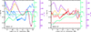 |
Fig. 5. Left: parameters along the line with maximum blueshifts. We show Doppler velocities from the polynomial fit (solid blue lines), Doppler velocities from the Fourier method (dashed blue), the magnetic inclination (green), the total magnetic field strength (violet), and the horizontal magnetic field strength (orange). Horizontal lines mark the zero reference for velocities (blue) and 90° for the magnetic inclination (green). Right: parameters for the maximum redshift. Here, the velocities are displayed in red. An animation of this figure is available online. |
| In the text | |
Current usage metrics show cumulative count of Article Views (full-text article views including HTML views, PDF and ePub downloads, according to the available data) and Abstracts Views on Vision4Press platform.
Data correspond to usage on the plateform after 2015. The current usage metrics is available 48-96 hours after online publication and is updated daily on week days.
Initial download of the metrics may take a while.