| Issue |
A&A
Volume 705, January 2026
|
|
|---|---|---|
| Article Number | A43 | |
| Number of page(s) | 13 | |
| Section | Stellar structure and evolution | |
| DOI | https://doi.org/10.1051/0004-6361/202452694 | |
| Published online | 06 January 2026 | |
A new sample of massive B-type contact binary candidates from the OGLE survey of the Magellanic Clouds
1
Instituto de Astrofísica de Canarias, Avenida Vía Láctea s/n, 38205 La Laguna, Santa Cruz de Tenerife, Spain
2
Universidad de La Laguna, Departamento de Astrofísica, Avenida Astrofísico Francisco Sánchez s/n, 38206 La Laguna, Santa Cruz de Tenerife, Spain
3
Department of Astronomy, 538 West 120th Street, Pupin Hall, Columbia University, New York City, NY 10027, USA
4
Lund Observatory, Division of Astrophysics, Department of Physics, Lund University, Box 43 SE-221 00 Lund, Sweden
5
Institute of Astronomy, Faculty of Physics, Astronomy and Informatics, Nicolaus Copernicus University, Grudziadzka 5, 87-100 Torun, Poland
6
Steward Observatory, Department of Astronomy, University of Arizona, 933 N. Cherry Ave, Tucson, AZ 85721, USA
7
Argelander Institut für Astronomie, Auf dem Hügel 71, DE-53121 Bonn, Germany
8
Max-Planck-Institut für Radioastronomie, Auf dem Hügel 69, DE-53121 Bonn, Germany
★ Corresponding author: This email address is being protected from spambots. You need JavaScript enabled to view it.
Received:
21
October
2024
Accepted:
1
October
2025
Abstract
Context. Massive contact binaries (CBs) are crucial objects for understanding close binary evolution and stellar mergers. Study of these objects has been hampered by a scarcity of observed systems, particularly of B-type systems which are expected to dominate this class.
Aims. We bridge this observational gap by mining a large sample of massive CB candidates from the OGLE-IV database, potentially increasing their current numbers in the Magellanic Clouds by an order of magnitude.
Methods. Using main-sequence color-magnitude limits, an observationally informed period-luminosity-color relation for CBs, and a high morph parameter cut (c ≥ 0.7), we empirically identified a subsample of 68 O and B-type binaries with periods P < 3 days, that exhibit smooth, sinusoidal light curves with nearly equal eclipse depths. To mine our bona fide sample of CB candidates among these, we used theoretical color-magnitude and orbital period distributions based on a vast grid of MESA binary models. We also computed synthetic light curves using PHOEBE corresponding to the contact and near-contact phases of a MESA model.
Results. Our bona fide candidate CB sample consists of 37 systems (9 in the SMC and 28 in the LMC), that fulfill the theoretical predictions for massive CBs. The bona fide sample, which predominantly consists of B-type binaries with periods of P ≈ 0.6 − 1 day, closely agrees with our predicted population count. As our binary models predict mass equalization followed by temperature equalization during nuclear-timescale contact, a substantial fraction of these bona fide CB candidates may have mass ratios of q ≈ 1.
Conclusions. Our work significantly expands the observational sample of B-type candidate massive CBs. Furthermore, our synthetic light curves show a degeneracy between contact and near-contact binary light curves, indicating the possibility of misidentifications between these configurations when characterized based on light curves alone. Spectroscopic follow-up is necessary to test our predictions, particularly for the mass ratios of these CB candidates.
Key words: binaries: close / binaries: eclipsing / binaries: general / stars: early-type / stars: evolution / stars: massive
© The Authors 2026
 Open Access article, published by EDP Sciences, under the terms of the Creative Commons Attribution License (https://creativecommons.org/licenses/by/4.0), which permits unrestricted use, distribution, and reproduction in any medium, provided the original work is properly cited.
This article is published in open access under the Subscribe to Open model. This email address is being protected from spambots. You need JavaScript enabled to view it. to support open access publication.
1. Introduction
Contact binaries (CBs) are a critical class of massive stars that allow us to examine how the closest binary stars evolve and what their end fates may be. In CBs, both stars overflow their Roche lobe volumes simultaneously and share a common envelope over nuclear timescales, rendering the contact phase as an observationally accessible phenomenon. At relatively high metallicities (Z ≥ ZSMC), massive CBs are expected to be the progenitors of stellar mergers of main-sequence (MS) binaries (Menon et al. 2021), while at lower metallicities, CBs may undergo chemically homogeneous evolution and become progenitors of black hole binaries (de Mink et al. 2009; Marchant et al. 2016). As members of triple systems at low metallicities, the CB channel can further contribute to the population of black hole binaries (Dorozsmai et al. 2024; Vigna-Gómez et al. 2025).
Intermediate luminosity transients such as luminous red novae (LRNe) are expected to be powered by stellar mergers. The most famous LRN resulted from the merger of V1309 Sco, a known low-mass CB (Tylenda et al. 2011; Tylenda & Kamiński 2016). More luminous LRNe may hence arise from the mergers of massive CBs. Thus, determining the number of CBs and their properties in an observable population allows the rate of MS stellar mergers and LRNe to be constrained and provides valuable tests for the formation pathways of compact-object binaries.
Menon et al. (2021, hereafter Paper I) built synthetic populations for the Large and Small Magellanic Clouds (LMC and SMC) from large grids of detailed binary models. They determined that massive CBs in the Magellanic Clouds will become MS binaries with mass ratios of q ≈ 1 and predominantly consist of B-type systems with periods ⪅1 day, due to their long contact durations and higher weight in the initial mass function (IMF). This theoretical probabilistic distribution of orbital parameters (P–q) was found to be similar within the metallicity range of the Magellanic Clouds.
Using archival records, Qian et al. (2007) and Abdul-Masih et al. (2022) determined the orbital period-change rates and thereby constrained the mass-transfer rates of massive-contact and near-contact O+O binaries. More recently, Vrancken et al. (2024) performed a similar analysis for five B+B systems, determining period-change rates with improved precision. These works concluded, within their uncertainties, that a subset of these systems are undergoing nuclear-timescale mass transfer, a finding broadly consistent with the prediction of Paper I.
The authors of Paper I had also compiled the first comprehensive list of spectroscopically confirmed massive CBs and near-CBs from the literature, i.e, those with radial velocity (RV) curves and light curves, comprising 26 systems in total from the SMC, LMC, and Milky Way (MW). The majority of these systems are in the MW and only two confirmed CBs have been identified in the Magellanic Clouds: OGLE SMC SC10-108086 (Hilditch et al. 2005), and VFTS 352 (Almeida et al. 2015). Collectively, this sample is also somewhat biased toward O-type systems with Teff ⪆ 30 kK and periods > 1 d. B-type CBs were largely underreported.
The field of massive CBs, thus, suffers from small-number statistics. To rigorously test theoretical predictions, a substantially larger, homogeneously analysed sample of massive CBs is required. Therefore for this work, we mined the largest photometric survey database of eclipsing binaries: the Optical Gravitational Lensing Experiment (OGLE)-IV survey of the Magellanic Clouds (Udalski et al. 2015; Pawlak et al. 2016). This survey comprises 40 204 eclipsing and ellipsoidal binaries in the LMC and 8401 in the SMC, and is largely complete for O and B-type MS binaries.
For paper, we first empirically selected a sample of O- and B-type MS binaries from the OGLE database that have smooth, sinusoidal light curves with nearly equal depths, resembling CBs with equal-temperature components. We further refined this sample using constraints from binary evolutionary models, which led to a “bona fide” sample of 37 massive CB candidates in total from the LMC and SMC, which we predict are the systems likeliest to be CBs. Our sample thus increases the number of known CBs in the Magellanic Clouds by an order of magnitude, making our sample the largest known homogeneous sample of CB candidates. The majority of this sample consists of B-type systems with periods of 0.6−1 days, thus remedying their deficit in existing literature. In addition, we also investigate the light curves of semi-detached and detached binaries nearing contact, compare them to those of CBs, and highlight potential observational misidentifications between these binaries.
This paper is divided as follows: In Section 2 we describe the empirical selection of our subsample of interest, Section 3.1 presents an exemplary binary evolution model, their corresponding light curves, and synthetic populations constructed from our binary model grid. In Section 4 we compare the empirical subsample and theoretical predictions to determine our bona fide CB candidate sample. In Section 5 we discuss the implications and caveats of our study, and place them in context with previous studies. Finally, in Section 6, we summarize the conclusions of our work.
2. Observational sample from OGLE
2.1. The OGLE massive main-sequence binary sample
The OGLE survey has been monitoring the Magellanic Clouds for over two decades. The fourth and current phase of the project began in 2010 and covers an area of about 650 square degrees, including the LMC, the SMC, and the Magellanic Bridge area between the two galaxies. The OGLE-IV observations were taken in Johnson’s V and Cousin’s I filters, with the majority (90%) of the observations taken in the I band. The OGLE-IV saturation limit in the I band is about 13 mag in the Magellanic Clouds. The survey has a high completeness level up to about 19 mag, however, some observations reach as faint as 21.5 mag. The technical details of the OGLE-IV survey can be found in Udalski et al. (2015).
The OGLE catalog reports the apparent V- and I-band magnitudes corresponding to the maximum brightness of the binary– at the peak amplitude of its light curve. We define MV, max and MI, max as the absolute V- and I-band magnitudes of the binary at its light curve maximum, i.e., when the system is at peak brightness and both stars are most visible. First, we de-reddened the individual OGLE sources using the optical reddening maps by Skowron et al. (2021). When comparing the values of E(V − I) implied by Skowron et al. (2021) for O-types stars in the LMC and SMC (selected from Bonanos et al. 2009, 2010, and other literature sources), we found small mean underestimates of 0.016 mag in the LMC and 0.0125 mag in the SMC compared to the spectroscopic reddening values. Therefore, assuming these offsets are also appropriate for massive binaries, we corrected E(V − I) by these values, before de-reddening the sample. We adopted RV, LMC = 3.4 for the LMC and RV, SMC = 2.74 for the SMC (Gordon et al. 2003).
Next, we corrected the de-reddened magnitudes for the distance modulus (DM) to obtain the absolute magnitudes. For this purpose, we adopted the DMLMC = 18.476 mag for the LMC (Pietrzyński et al. 2019) and DMSMC = 18.997 mag for the SMC (Graczyk et al. 2020). Stars in the Magellanic Clouds are generally too far away to have good parallax measurements in Gaia, so any object that has a positive parallax and parallax/parallax-error greater than five must be a Galactic foreground object and not an LMC or SMC member. We used Gaia DR3 parallax data (Gaia Collaboration 2021) to remove these foreground objects from our sample.
We filtered the massive MS binaries from this de-reddened sample using zero Age Main Sequence (ZAMS) and terminal Age Main Sequence (TAMS) color-magnitude diagram (CMD) limits. These limits were determined using absolute V-band magnitudes and absolute V-I colors for LMC single-star models with masses ranging from 7 to 50 solar masses (M⊙) and two initial rotational velocities: vi = 0 km/s and vi = 330 km/s, computed using MESA v. r15140 (Paxton et al. 2011, 2013, 2015; Paxton et al. 2018), which provides bolometric luminosities only. To convert these to absolute V- and I-band magnitudes, we employed the bolometric corrections and colors from the TLUSTY O- and B-star model atmosphere grids (Lanz & Hubeny 2003, 2007).
Figure 1 illustrates the resulting absolute CMD. The theoretical ZAMS and TAMS curves of the MS tracks on the CMD indicate that massive MS binary systems containing stars with initial masses 7 M⊙ have absolute V-band magnitudes of MV ⪆ −2.5, absolute V-I colors of −0.307 ⪅ MV − MI ⪅ −0.165. The OGLE binaries within the above limits are likely to be massive MS binaries, corresponding roughly to spectral types B2 V and earlier according to the classification scheme of Pecaut & Mamajek (2013). Some points fall outside these limits; however, cross-matching the OGLE sample with known OB systems indicates that these are likely the result of incorrect extinction corrections derived from the Skowron et al. (2021) maps that are of low spatial resolution. In total, we obtained 2811 and 861 early MS binaries in the LMC and SMC, respectively, with orbital periods P < 30 days.
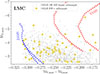 |
Fig. 1. OB binaries with periods P ≤ 3 days across all morph parameter values (from 0 to 1), identified as MS systems from the OGLE sample (light grey dots) on the absolute color (MV, max − MI, max) – magnitude (MV, max) space (where, the absolute magnitudes correspond to their values at maximum brightness of the binary). Overlaid are the empirically identified OGLE EW+ subsample from the LMC (yellow circles, as described in Section 2.2). Curves indicate the limits of the ZAMS and TAMS curves computed from non-rotating and rotating (vi = 330 km/s) models of single stars with masses of 7 − 50 M⊙. |
We also examined the binary number statistics and the completion of our sample selection for CBs. For this, we use the Gaia catalog to estimate the total number of MS stars in each galaxy that lie within the OGLE binary survey spatial and color-magnitude footprints (for a discussion of the completeness of Gaia see Schootemeijer et al. 2021). Reassuringly, both the LMC-to-SMC ratios of OGLE binaries and Gaia MS are nearly identical over an absolute magnitude range corresponding to spectral types O9/B0 V (MV ∼ −5) to approximately B7 V (MV ∼ −1), as can be seen in Fig. 2. For the brightest magnitudes the OGLE survey suffers from incompleteness close to the saturation limits (around MV, max ∼ −6.0 in the LMC and MV, max ∼ −6.4 in the SMC) and stochastic effects (small numbers of stars). In addition, the incompleteness due to faint limits impacts both OGLE and Gaia at different absolute magnitudes. Assuming detection biases are roughly the same in OGLE for both the LMC and SMC, Fig. 2 implies that binary fractions of late O- and B-type stars in both galaxies are roughly the same, indicating a metallicity independence in their distribution. This is consistent with the findings of Paper I, where a similar result for the population of CBs in both Magellanic Clouds was found. While the ratios are similar, the trend of the OGLE binary fraction relative to Gaia MS stars exhibits a drop from around 10% to a few percent at fainter magnitudes. We expect this decrease to be driven primarily by an observational bias: lower signal-to-noise light curves make it increasingly difficult to identify binaries at lower luminosities. In addition, there may be a genuine physical trend, with the intrinsic binary fraction decreasing toward lower masses (Banyard et al. 2022).
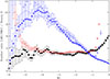 |
Fig. 2. Characterization of the OGLE binary sample. The black filled circles represent the ratio of LMC to SMC OGLE binaries, red circles are the same ratio but for Gaia MS stars, and blue triangles are the percentage binary fractions (OGLE/Gaia) for the LMC (filled triangles) and SMC (open triangles). The x-axis represents the absolute V-band magnitude MV (or MV, max in the case of OGLE binaries). Error bars represent Poisson uncertainties |

The average recall of the classifier used in Pawlak et al. (2016) is about 80%, and is likely to be slightly higher for the early-type contact binaries, as they are bright and therefore have lower scatter than most of the sample. The main limiting factor for the completeness is the inclination of the system. Roughly half of the population of CBs may not show eclipses due to low inclination of the orbit. Some of these systems may be detected as ellipsoidal (ELL) binaries, though. A second limiting factor is the OGLE saturation limit, which excludes the brightest O-type stars (apparent magnitude ⪅13.2).
2.2. Empirical OGLE EW+ subsample
We used the empirical period-luminosity-color (PLC) relation for CBs from Pawlak (2016), to calculate the period of the widest O-type CBs. For an O4V-type MS CB, this is ∼3 days. We note that there is significant scatter in this relation, therefore, this is only a rough estimate of the upper period limit for massive CBs.
Light curves are conventionally classified as: smooth sinusoidal light curves with both eclipses having equal or very similar depths EW, light curves with barely-visible distinction between the eclipse and out-of-eclipse phase but unequal depths EB, light curves with flat-bottomed minima and a clearer distinction between the eclipse and out-of eclipse phase EA and, smooth, sinusoidal light curves without eclipses, where only ellipsoidal modulation is visible ELL. These ELLs typically arise from binaries viewed at low inclinations, making their intrinsic geometric configurations highly uncertain. Examples of EW, EB and ELL light curves from the OGLE database are shown in Fig. 3.
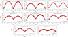 |
Fig. 3. Exemplary I-band light curves from the OGLE database, classified by this study as EW (top), EB (middle) and ELL (bottom). The OGLE database itself uses a different classification scheme. |
In the OGLE database, however, light curves are not classified following these conventions. They were visually classified into three types – contact (C), non-contact (NC), and ellipsoidal (ELL) – within our period range of interest. The label “C” indicates systems with EW light curves; however, since these light curves were classified by eye, they were prone to errors. We therefore discarded the OGLE labels, and systematically selected binaries with light curves suited for our study.
Our primary assumption for selecting contact systems is that they are MS binaries with EW-type light curves, wherein nearly equal eclipse depths imply nearly equal temperature components. This is because the eclipse-depth ratio is proportional to the fourth power of the temperature ratio of its components, (T2/T1)4, or, alternatively, their relative eclipse depth, fΔA ∝ (T2/T1)4. We define the relative eclipse depth as,  , where A1 and A2 represent the difference between the magnitude of the binary at maximum brightness, and the primary and secondary eclipse minima, respectively. Thus for the strict definition of EW light curves, fΔA ∼ 0. However, since there are spectroscopic CBs reported with (T2/T1) slightly away from one, we relaxed this requirement for strictly equal minima and included systems whose light curves show a nominal difference in eclipse depths, namely, with fΔA ≤ 0.1. Within this constraint on eclipse depths, the radii ratio can be reasonably neglected.
Next, we filtered the sample based on their morph-parameter value provided by Bódi & Hajdu (2021) for the above categories of light curves in the OGLE-IV catalog. The morph parameter quantifies the geometric smoothness of the light curve shape and is a continuous value in the range 0 < c < 1; the smoother the light curve is, the closer c is to one (Prša et al. 2008). Bódi & Hajdu (2021) found that EW light curves have c ⪆ 0.68 (see their Fig. 1). Hence, we set a limit of c ≥ 7, to obtain systems with smooth sinusoidal light curves.
To summarize, our empirical criteria for the OGLE EW+ subsample which also includes binaries with slightly asymmetric light curves, are:
-
They must have a high morph parameter (c ≥ 0.7).
-
They must have orbital periods ≤3 days, according to the empirical PLC of Pawlak et al. (2016).
-
Their absolute V-band magnitude is MV, max ⪅ −2.5 and the absolute V-I color is −0.307 ⪅ MV, max − MI, max ⪅ −0.165.
-
The ELL binaries are excluded as their geometric configuration cannot be reliably determined.
-
The relative eclipse depth between the primary and secondary components is fΔA ⪅ 0.1.
Out of 2811 LMC and 861 SMC MS binaries, 56 systems in the LMC and 24 systems in the SMC satisfy these empirical criteria, and subsequently form our OGLE EW+ sample. Critically, these photometric–morphology criteria were defined prior to any reference to our synthetic CB predictions. This separation ensures that the empirically selected sample remains independent of theoretical expectations, which we describe in the next section.
3. Synthetic light curves and populations of massive contact binaries
3.1. Binary evolution
In our binary models, we defined the contact and near-contact phases based on the Roche lobe fill-out factors of the component stars, calculated as the ratio of their volume-equivalent radius to their Roche-lobe radius (R/RRL). During the contact phase both stars have R/RRL > 1, and in the near-contact phase they have R/RRL = 0.9 − 1.0, following the same nomenclature as Paper I.
In Paper I, two pathways to achieving nuclear-timescale contact were elucidated: the “System 1” channel, where binaries achieved early contact, just after the zero-age MS (ZAMS) and sustain contact until the binary overflows through the L2 Lagrangian point, and the “System 2” channel, in which binaries acquired delayed contact after a semi-detached phase. System 1 binaries dominate synthetic CB populations due to their significantly longer contact durations than System 2 binaries. However, System 2 binaries offer the opportunity to self-consistently study both the near-contact and contact phases, and examine the transition in light curve morphology between these phases.
Figure 4 provides an overview of the evolution of the exemplary System 2 of Paper I, with initial parameters, MT, i = 26 M⊙, Pi = 1.0 d, qi = 0.8, computed with MESA v.10398 (Paxton et al. 2011, 2013, 2015). On achieving nuclear-timescale contact at ≈6.4 Myr, this system evolves towards an equal-mass binary (q ≈ 1). The nuclear timescale contact results in temperature equalization following mass equalization, i.e., T2/T1 ≈ 1 as q → 1, as seen in panel 2 of Fig. 4.
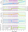 |
Fig. 4. Panels showing the evolution of the exemplary ‘System 2’ binary model from Paper I, with initial parameters: MT, i = 26 M⊙, Pi = 1.0 d, and qi = 0.8. The parameters from top to bottom panels are: the fill-out factor (R/RRL), the temperature and mass ratio (T2/T1; q), orbital period (P), mass of both components and the mass-transfer rate. Also shown are the contact (light-green region) phase and near-contact (pink region) phase, which is further divided into the detached phase (crosshatching) and semi-detached phase (striped hatching). The open circles are the instances at which synthetic PHOEBE light curves are computed (Fig. 5). |
This model, as with all others in this paper, does not include energy transfer within the shared envelope. Although the inclusion of envelope heat-transfer can increase the time spent in the q < 1 phase during contact (Fabry et al. 2023), its overall impact on the parameter distribution of a population is minor (Fabry et al. 2025). We discuss this point later in Section 5.
As the binary approaches contact, the system is first a detached system and later, a semi-detached system. The binary spends ≈4.4 Myr in this near-CB phase, which is about 1.5 times longer than its contact phase, while maintaining a mass ratio of q < 1, demonstrating that a mere 10% difference in the Roche lobe fill-out factor results in a distinctly different structural configuration. As we show in Section 4, such near-contact binaries (near-CBs) are expected to be more numerous than CBs due to their longer evolutionary timescales and typically have longer orbital periods, of ≈1 − 2.5 days.
3.2. Synthetic binary light curves
We next investigated how the light curve of this binary behaves at different instances of its evolution at the time stamps indicated in Fig. 4. We computed synthetic light curves using PHOEBE II (hereafter PHOEBE; Prša et al. 2016; Horvat et al. 2018; Jones et al. 2020; Conroy et al. 2020), which is based on the Wilson–Devinney code (Wilson & Devinney 1971). We assumed a blackbody atmosphere for both stars, which provides a simplified but sufficient approximation for the purpose of light curve morphology. To compute the light curves, we supplied the mass ratio (q), temperatures T1, T2, orbital period (P), inclination (i), primary mass and radius of the secondary at each time-stamp of System 2 indicated in Fig. 4.
Figure 5 shows the resulting PHOEBE light curves. We find that the light curves are most sensitive to the inclination angle, the temperature ratio, and Roche-lobe fill-out factors (R1/RRL, 1, R2/RRL, 2). At high inclination angles, close to 90°, the configuration of the binary can be reliably inferred from the light curve shape with minimal uncertainty.
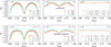 |
Fig. 5. Light curves computed for System 2 at the various evolutionary points marked in Fig. 4, at inclinations of i = 30°, 60° and 90°. Top panel: Light curves from the contact phase (green region in Fig. 4), where the cyan light curve represents the dominant type of CB expected from models, i.e., one which has acquired temperature equalization. Bottom panel: Light curves during the near-contact phase CB (pink striped region in Fig. 4), which is further split as a semi-detached (red and orange light curves) and detached system (cyan light curve). Also labeled are the relative eclipse depths, fΔA, except for ELL binaries, which have an fΔA of the order of 0.001. |
In the contact phase, the model has fill-out factors of R/RRL = 1.1 − 1.2 for both components and is predominantly a binary with T1 ≈ T2 and q ≈ 1. The corresponding EW PHOEBE light curves have relative eclipse depths of fΔA ≈ 0.09 − 0.009, as the inclination lowers from 90° to 60°.
In the phase prior to attaining contact, the binary is a semi-detached or detached binary system nearing contact. The corresponding synthetic EB light curves have relative eclipse depths of fΔA = 0.145 − 0.241, as the mass ratio of the model in this phase is q ≈ 0.71 − 0.84. These EB light curves are visually similar to EW light curves except for their larger values of fΔA, which may lead to their interpretation as belonging to unequal-mass CBs with q < 1; examples of such systems may include V382 Cyg and TU Mus.
Distinguishing contact from near-contact binaries becomes even more challenging at lower inclinations. As the inclination angle approaches 60°, we find an increasing degeneracy between the light curves of the binary during the contact and near-contact phase. Even while the intrinsic T2/T1 ≠ 1, the eclipse depth ratio approaches one, or in other words, the relative eclipse depth, fΔA decreases up to 0.072 at 60°. Thus as the inclination angle decreases, near-CBs can have EW/ELL-type light curves, which lends them the impression of being CBs with nearly equal eclipse depths, although their intrinsic temperature ratio is T2/T1 < 1. At i = 30° the situation worsens with an fΔA of the order of 0.001, as only the ellipsoidal modulations of the binary are visible in the light curve, making it exceptionally challenging to discern the configuration of the binary. Thus a near-CB with a mass and temperature ratio of less than one, could be classified as having an EW/ELL light curve (Fig. 3) at moderate-to-low inclinations.
Thus, while a fill-out factor of 10% can result in a completely different evolutionary configuration of the binary, their light curves, especially at moderate to low inclinations, are not sensitive to this difference and are nearly indistinguishable between contact and near-contact binaries. To summarise:
-
Near CBs at moderate to low inclinations (i ⪅ 60°) can exhibit light curves with nearly equal-eclipse depths, and become misclassified as CBs with EW light curves, particularly at P ≳ 1 days.
-
Near CBs with smooth light curves that have sharp minima and unequal eclipse depths at high inclinations, could also be misinterpreted as CBs with T2 < T1 and possibly q < 1.
-
At extremely low inclinations (i ⪅ 30°), only ellipsoidal variability is visible in the light curve (ELL), making the intrinsic binary configuration difficult to determine.
These degeneracies between contact and near-contact binaries can be somewhat alleviated by studying synthetic populations and their parameter distributions.
3.3. Binary-model grids and synthetic populations
We combined two grids of models in this work: the “Menon grid” from Paper I for binaries with initial periods of 0.6 − 2 days and the “Bonn grid” (Marchant 2017; Sen et al. 2022), spanning 2.1 − 3162 days using MESA (Paxton et al. 2011, 2013, 2015, 2018, 2019). In this work, we extended the Menon grid to ensure full coverage of B-type binaries by computing new models with initial masses of MT, i = 14…18 M⊙. Table 1 summarizes the parameters and relative weights of each grid. These parameters reflect the parameter space coverage for massive binaries, based on the findings of Sana et al. (2013) of 30 Doradus, from the VLT-FLAMES Tarantula survey (Evans et al. 2011). Thereafter, using the same assumptions and methods as Paper I, we constructed synthetic populations from this combined model grid and computed the parametric probability distributions (further described in Appendix A).
Parameters of the two grids of binary models used in this work.
Paper I had shown that the distributions of binary properties are similar for the metallicities of the LMC and SMC for our systems of interest. In Section 2.1, we also found that the binary fraction at different luminosities is similar between the LMC and SMC. Therefore, we constructed the probability distributions only for the LMC and adapted the distributions to the SMC by scaling it to the number of massive MS binaries in the SMC. Case-A mass transfer is expected to occur in binaries with initial orbital periods up to Pi ≈ 23 days, which defines the upper limit for systems contributing to the contact and near-contact binary populations. The number of systems calculated from our synthetic populations (the details of which are in Appendix A) are:
Near-CBs are predicted to be nearly twice as common as contact systems in a population, making them more likely to be observed. The predicted counts of 39 CBs in the LMC and 12 in the SMC serve as benchmarks for comparison with the OGLE sample.
We note that the contribution to the CB population solely originates from the Menon grid, i.e., from binaries with initial periods under 2 days. Including the Bonn grid effectively broadens the parameter space over which near-CBs may be observed compared to Paper I, as we discuss in the next section.
4. Comparing massive CB candidates with theoretical populations
We investigated synthetic distributions for three properties from the OGLE catalog: the absolute magnitude (MV, max), color (MV, max − MI, max), and orbital period (P). Models from MESA provide the intrinsic luminosities of the binary components, whose sum corresponds observationally to the maximum absolute brightness of the system at an inclination of i = 90°. We first converted the bolometric luminosities of the primary and secondary stars in each binary model to their respective absolute V- and I-band magnitudes using the flux–magnitude relation and bolometric corrections from Section 2.1. We then reconverted the V- and I-band magnitudes of each stellar component into their intrinsic luminosities, computed the total binary luminosity in each band (Lbinary, band = L1, band + L2, band), and finally converted Lbinary, band to the absolute V- and I-band magnitudes of the binary (MV, max and MI, max) using the flux–magnitude relation once more.
Figure 6 shows the location of our OGLE EW+ sample on the theoretical CMD. The B-type CBs appear more evolved than the O-type CBs–likely because their longer contact durations allow them to remain on the MS longer before merging. A few OGLE systems are bluer than our theoretical ZAMS curves, suggesting an overestimated extinction (as noted in Section 2.1). Overall, the locations of our mined OGLE sample agree well with the theoretical CMD for massive CBs.
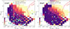 |
Fig. 6. Heat map showing the probabilistic distribution of the absolute color (MV, max − MI, max) and magnitude (MV, max) at the maximum brightness (i.e., the sum of intrinsic luminosities of both components) of CBs for the LMC and SMC. The OGLE data are marked as follows: OGLE bona fide CB sample (blue diamonds), OGLE EW+ subsample (yellow circles) and OGLE Rest (grey dots), which is the sample with morph parameter c > 0.7 and P ≤ 3 days that did not make the cut into either the EW+ nor the bona fide CB sample. For reference, the theoretical ZAMS and TAMS curves from Fig. 1 are also marked. |
Figure 7 shows the probability distributions for CBs from our binary model grid in the period–magnitude plane, together with our empirical OGLE EW+ sample (yellow circles), and all other high-morph parameter binaries occupying the same period–color–magnitude domain but with larger relative eclipse depths fΔA > 0.1 (grey dots). Although the empirical PLC extends to P ≈ 3 days, our OGLE EW+ sample shows clear outliers beyond 2 days, thus deviating from the expected trend and suggesting that the PLC relation may not reliably apply to massive systems in this period regime.
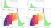 |
Fig. 7. Heat map showing the probabilistic distribution of the absolute magnitude (MV, max) at maximum brightness to orbital period (P) of CBs, for the LMC and SMC. O- and B-type systems are distinguished by a magnitude cutoff at MV, max = −4. The OGLE data are annotated as in Fig. 6. For reference, the theoretical extent of the bona fide CB sample is indicated by the polygon outlined in blue dots, beyond which their number counts from de-convoluted histograms (green histograms) drop below one. |
The high-likelihood region for CBs, indicated by the blue polygon in Fig. 7, extends to P ≈ 1.2 days in the LMC and P ≈ 1.0 days in the SMC– these represent the widest CBs expected from our models. Beyond this limit the population count for CBs is smaller than 1. Systems falling within this region form our “bona fide CB sample”. This sample comprises 28 CB candidates in the LMC and 9 candidates in the SMC. Of these 37 systems, 27 are B-type binaries with orbital periods of 0.6−1.0 days. This sample also includes the two known spectroscopic CBs in the Magellanic Clouds– VFTS 352 (Almeida et al. 2015) in the LMC and OGLE SMC-SC10 108086 system (Hilditch et al. 2005). The full set of bona fide CB candidates and the extended EW+ sample are listed in Tables B.1 and B.2.
For comparison with the theoretical population counts (Section 3.3), we also considered the broader census of EW+ binaries (including the bona fide sample) and ELL binaries within the high-likelihood region of CBs, yielding:
These numbers are remarkably close to our theoretical estimates from Section 3.3, indicating a consistency between the data and theory. The period, magnitude and color distributions of the bona fide sample shown in Figs. 7 and B.1 are consistent with the CB population predicted from our MESA models. Our prediction from Fig. B.1 for this mined sample is that these binaries are likely to have mass ratios of q ≈ 1. Further spectroscopic follow-up with RV data is required to confirm our prediction.
Figure B.1 also shows that near-CBs are expected to be twice as numerous as CBs and have orbital periods of ∼1 − 2.5 days and mass ratios of q ≈ 0.4 − 1. This orbital period limit is longer than the number predicted in Paper I due to the inclusion of the Bonn grid in our work. A fraction of these systems may have light curves similar to CBs, as demonstrated in Section 3.2, and masquerade as CBs with P ⪆ 1 days in a population.
5. Discussion
We empirically mined 56 LMC and 24 SMC massive MS binaries from the OGLE survey with EW light curves, indicating these systems have nearly equal temperature components. Of these, 28 LMC systems and 9 SMC systems form our bona fide contact binary (CB) candidate sample, making the largest homogeneous sample of massive CB candidates in literature. Including ELL binaries would further increase this sample, and bringing the sample size strikingly close to our predicted number of CBs: 39 and 12 systems in the LMC and SMC respectively. Accounting for the OGLE survey’s ∼80% classifier recall suggests that the underlying population of massive CBs may be even larger, and thus we may be missing about 20% of systems from our mined sample. Conversely, incorporating the detailed star-formation histories of the Magellanic Clouds may instead reduce these estimates. During the preparation of this manuscript, OGLE released an updated database (Głowacki et al. 2024), the consideration of which may further affect the above numbers.
Our models suggest that the bona fide CB candidates are likely undergoing a nuclear-timescale contact phase, during which mass equalization leads to subsequent temperature equalization. According to our synthetic populations, such q ≈ 1 CBs are expected to dominate the overall census of massive CBs. This result is further reinforced by the recent work of Fabry et al. (2025), who included additional physics such as envelope energy transport and tidal deformation in their CB models (which were not included in our models). By building synthetic populations with their models, they inferred that while heat-transfer physics allows for a minority population (⪅10%) of delayed-contact CBs with q < 1, the dominant majority of CBs remain as B-type binaries that attain contact soon after ZAMS. Therefore, even with the inclusion of these physics mechanisms, the P − q distribution of massive CBs remains dominated by q ≈ 1 systems with periods less than 1 day, consistent with our predictions from Paper I and this work.
Such equal-mass CBs are not uncommon in the literature. Of the two previously reported spectroscopic CBs in the Magellanic Clouds, the deep-contact binary VFTS 352 (Almeida et al. 2015; Mahy et al. 2020), which is also part of our OGLE sample, has a mass ratio of q ≈ 1. The sole spectroscopic CB reported in the SMC, OGLE SMC SC10-108086 (Hilditch et al. 2005), is also part of our sample. Its reported mass ratio of  , suggests that this system can have a mass ratio up to q = 0.91, which though not exactly equal to one, is close to a mass ratio of unity. B-type spectroscopic binaries in deep contact in the MW also have equal-mass components, as do two recent photometric systems discovered in the M31 galaxy (Li et al. 2022). VFTS 066 was earlier classified as a CB in Mahy et al. (2020), however, this system has an inclination of i = 17.5° and only shows ellipsoidal variability (Vrancken et al. 2024). Thus its intrinsic configuration cannot be definitively ascertained.
At this juncture, we wish to emphasize that the compendium of spectroscopic systems presented in Paper I represents a mixed population, with many q < 1 systems occupying ambiguous contact or near-contact configurations. Indeed, our PHOEBE models demonstrate that contact and near-contact configurations can be degenerate, implying that a fraction of near-CBs with smooth EW light curves could be mistaken for contact systems, especially at low inclinations. We encourage that a given system in the sample compendium of Paper I be carefully assessed to be interpreted as a q < 1 semi-detached or detached binary to avoid overstating the likelihood of genuine CBs with q < 1 CBs.
A close examination of the literature reporting q < 1 CBs, revealed that the uncertainty in their Roche lobe fill-out factor allows for their interpretation also as binaries only approaching contact. Examples of such systems include V382 Cyg (Yaşarsoy & Yakut 2013; Martins et al. 2017), TU Mus (Penny et al. 2008) and LSS 3074 (Raucq et al. 2017), which have been described as “marginally in contact”, “shallow contact”, or “approaching contact”, highlighting the ambiguity in the configuration of reported contact systems. Based on analysis of spectroscopic and photometric data, V729 Cyg (Yaşarsoy & Yakut 2014) and V382 Cyg (Yaşarsoy & Yakut 2013; Martins et al. 2017) can be classified either as a binary in “weak” contact, barely filling its Roche lobes, or as a semi-detached binary nearing contact. V729 Cyg may in fact not even be a MS binary, but a system containing a Wolf-Rayet star. These uncertainties in fill-out factors, coupled with the presence of such atypical systems, suggest that the existing sample in the literature likely represents a mixed population of contact and near-contact binaries, with near-contact systems expected to be about twice as common as contact systems, according to our findings.
We do not preclude the possibility of q < 1 massive CBs, nor make predictions for their population counts, which is beyond the scope of this study. A fraction of these q < 1 systems may be included in our sample, since we also accommodate systems with slightly unequal temperatures, and therefore possibly, unequal masses. We also do not rule out the existence of CBs with periods longer than 1.2 days, which are included in the “extended sample” of systems in Tables B.1 and B.2. A multi-epoch spectroscopy campaign is essential to determine the mass ratios of our sample.
6. Conclusions
We have identified a total of 37 bona fide CB candidates from the Magellanic Clouds, with nearly equal eclipse depths, which may be associated with binaries containing equal-temperature components. Notably, this sample also contains 27 B-type systems, thus addressing the long-standing dearth of B-type CBs and equal-temperature CBs in the literature. Along with ten O-type systems (of which two were previously known), we have increased the number of massive CB candidates in the Magellanic Clouds, by an order of magnitude. Incorporating additional ELL-type binaries brings the sample into close agreement with our theoretical predictions. However, classification uncertainties and the underlying star-formation histories may affect the true population size of CBs.
Our theoretical models and synthetic light curves suggest that these CB candidates may have undergone mass equalization prior to achieving temperature equalization. Therefore, we expect a subset of the sample to represent the previously underreported population of q ≈ 1 massive CBs.
The synthetic light curves we constructed for evolutionary models of semi-detached and detached systems nearing contact were found to be similar to CBs, except for their distinctly unequal eclipse depths. This morphological similarity may lead to the misidentification of some near-CBs as CBs with highly unequal mass components, which becomes more pronounced at low inclinations. Thus, a 10% difference in the Roche lobe fill-out factor, which appears modest from an observational perspective, can mask critical differences in physical configuration and result in observational ambiguity between contact and near-contact states.
Our theoretical predictions and candidate CB sample suggest that massive contact binaries comprise about 1−2% of the massive MS binary population. Despite their small numbers, these systems represent an important population, which can serve as an observational portal into the understudied channel of binary evolution involving stellar mergers and in extremely metal-poor environments, a pathway towards chemically homogeneous evolution and thereafter towards q = 1 black hole binaries. Furthermore, our study establishes a promising pipeline that connects binary evolutionary models with their predicted light curves and leverages this combined output to mine photometric surveys and multi-epoch radial-velocity data from spectroscopic surveys such as the BLOeM survey (Shenar et al. 2024) and the upcoming 4MOST survey (Cioni et al. 2019; de Jong et al. 2019). Deep learning techniques and machine-learning classifications, will further develop this pipeline and enable full-fledged population studies of various binary classes and the distribution of their properties.
Acknowledgments
AM was supported by the Juan de la Cierva Incorporación fellowship IJC2020-045628-I for this work. MP is supported by the BEKKER fellowship BPN/BEK/2022/1/00106 from the Polish National Agency for Academic Exchange and the Royal Physiographic Society in Lund through the Märta and Erik Holmbergs Endowment. We thank Michael Abdul-Masih for their help with PHOEBE and Artemio Herrero for insightful discussions that helped shape this paper.
References
- Abdul-Masih, M., Escorza, A., Menon, A., Mahy, L., & Marchant, P. 2022, A&A, 666, A18 [NASA ADS] [CrossRef] [EDP Sciences] [Google Scholar]
- Almeida, L. A., Sana, H., de Mink, S. E., et al. 2015, ApJ, 812, 102 [Google Scholar]
- Banyard, G., Sana, H., Mahy, L., et al. 2022, A&A, 658, A69 [NASA ADS] [CrossRef] [EDP Sciences] [Google Scholar]
- Bódi, A., & Hajdu, T. 2021, ApJS, 255, 1 [CrossRef] [Google Scholar]
- Bonanos, A. Z., Massa, D. L., Sewilo, M., et al. 2009, AJ, 138, 1003 [Google Scholar]
- Bonanos, A. Z., Lennon, D. J., Köhlinger, F., et al. 2010, AJ, 140, 416 [NASA ADS] [CrossRef] [Google Scholar]
- Cioni, M. R. L., Storm, J., Bell, C. P. M., et al. 2019, The Messenger, 175, 54 [NASA ADS] [Google Scholar]
- Conroy, K. E., Kochoska, A., Hey, D., et al. 2020, ApJS, 250, 34 [Google Scholar]
- de Jong, R. S., Agertz, O., Berbel, A. A., et al. 2019, The Messenger, 175, 3 [NASA ADS] [Google Scholar]
- de Mink, S. E., Cantiello, M., Langer, N., et al. 2009, A&A, 497, 243 [NASA ADS] [CrossRef] [EDP Sciences] [Google Scholar]
- Dorozsmai, A., Toonen, S., Vigna-Gómez, A., de Mink, S. E., & Kummer, F. 2024, MNRAS, 527, 9782 [Google Scholar]
- Dunstall, P. R., Dufton, P. L., Sana, H., et al. 2015, A&A, 580, A93 [NASA ADS] [CrossRef] [EDP Sciences] [Google Scholar]
- Evans, C. J., Taylor, W. D., Hénault-Brunet, V., et al. 2011, A&A, 530, A108 [NASA ADS] [CrossRef] [EDP Sciences] [Google Scholar]
- Fabry, M., Marchant, P., Langer, N., & Sana, H. 2023, A&A, 672, A175 [NASA ADS] [CrossRef] [EDP Sciences] [Google Scholar]
- Fabry, M., Marchant, P., Langer, N., & Sana, H. 2025, A&A, 695, A109 [NASA ADS] [CrossRef] [EDP Sciences] [Google Scholar]
- Gaia Collaboration (Brown, A. G. A., et al.) 2021, A&A, 649, A1 [NASA ADS] [CrossRef] [EDP Sciences] [Google Scholar]
- Głowacki, M., Soszyński, I., Udalski, A., et al. 2024, Acta Astron., 74, 241 [Google Scholar]
- Gordon, K. D., Clayton, G. C., Misselt, K. A., Landolt, A. U., & Wolff, M. J. 2003, ApJ, 594, 279 [NASA ADS] [CrossRef] [Google Scholar]
- Graczyk, D., Pietrzyński, G., Thompson, I. B., et al. 2020, ApJ, 904, 13 [Google Scholar]
- Hilditch, R. W., Howarth, I. D., & Harries, T. J. 2005, MNRAS, 357, 304 [NASA ADS] [CrossRef] [Google Scholar]
- Horvat, M., Conroy, K. E., Pablo, H., et al. 2018, ApJS, 237, 26 [Google Scholar]
- Jones, D., Conroy, K. E., Horvat, M., et al. 2020, ApJS, 247, 63 [Google Scholar]
- Lanz, T., & Hubeny, I. 2003, ApJS, 146, 417 [NASA ADS] [CrossRef] [Google Scholar]
- Lanz, T., & Hubeny, I. 2007, ApJS, 169, 83 [CrossRef] [Google Scholar]
- Li, F. X., Qian, S. B., Jiao, C. L., & Ma, W. W. 2022, ApJ, 932, 14 [NASA ADS] [CrossRef] [Google Scholar]
- Mahy, L., Almeida, L. A., Sana, H., et al. 2020, A&A, 634, A119 [NASA ADS] [CrossRef] [EDP Sciences] [Google Scholar]
- Marchant, P. 2017, Ph.D. Thesis, Rheinische Friedrich Wilhelms University of Bonn, Germany [Google Scholar]
- Marchant, P., Langer, N., Podsiadlowski, P., Tauris, T. M., & Moriya, T. J. 2016, A&A, 588, A50 [NASA ADS] [CrossRef] [EDP Sciences] [Google Scholar]
- Martins, F., Mahy, L., & Hervé, A. 2017, A&A, 607, A82 [NASA ADS] [CrossRef] [EDP Sciences] [Google Scholar]
- Menon, A., Langer, N., de Mink, S. E., et al. 2021, MNRAS, 507, 5013 [NASA ADS] [CrossRef] [Google Scholar]
- Pawlak, M. 2016, MNRAS, 457, 4323 [CrossRef] [Google Scholar]
- Pawlak, M., Soszyński, I., Udalski, A., et al. 2016, Acta Astron., 66, 421 [Google Scholar]
- Paxton, B., Bildsten, L., Dotter, A., et al. 2011, ApJS, 192, 3 [Google Scholar]
- Paxton, B., Cantiello, M., Arras, P., et al. 2013, ApJS, 208, 4 [Google Scholar]
- Paxton, B., Marchant, P., Schwab, J., et al. 2015, ApJS, 220, 15 [Google Scholar]
- Paxton, B., Schwab, J., Bauer, E. B., et al. 2018, ApJS, 234, 34 [NASA ADS] [CrossRef] [Google Scholar]
- Paxton, B., Smolec, R., Schwab, J., et al. 2019, ApJS, 243, 10 [Google Scholar]
- Pecaut, M. J., & Mamajek, E. E. 2013, ApJS, 208, 9 [Google Scholar]
- Penny, L. R., Ouzts, C., & Gies, D. R. 2008, ApJ, 681, 554 [Google Scholar]
- Pietrzyński, G., Graczyk, D., Gallenne, A., et al. 2019, Nature, 567, 200 [Google Scholar]
- Prša, A., Guinan, E. F., Devinney, E. J., et al. 2008, ApJ, 687, 542 [CrossRef] [Google Scholar]
- Prša, A., Conroy, K. E., Horvat, M., et al. 2016, ApJS, 227, 29 [Google Scholar]
- Qian, S. B., Yuan, J. Z., Liu, L., et al. 2007, MNRAS, 380, 1599 [NASA ADS] [CrossRef] [Google Scholar]
- Raucq, F., Gosset, E., Rauw, G., et al. 2017, A&A, 601, A133 [NASA ADS] [CrossRef] [EDP Sciences] [Google Scholar]
- Sana, H., de Koter, A., de Mink, S. E., et al. 2013, A&A, 550, A107 [NASA ADS] [CrossRef] [EDP Sciences] [Google Scholar]
- Schootemeijer, A., Langer, N., Lennon, D., et al. 2021, A&A, 646, A106 [NASA ADS] [CrossRef] [EDP Sciences] [Google Scholar]
- Sen, K., Langer, N., Marchant, P., et al. 2022, A&A, 659, A98 [NASA ADS] [CrossRef] [EDP Sciences] [Google Scholar]
- Shenar, T., Bodensteiner, J., Sana, H., et al. 2024, A&A, 690, A289 [NASA ADS] [CrossRef] [EDP Sciences] [Google Scholar]
- Skowron, D. M., Skowron, J., Udalski, A., et al. 2021, ApJS, 252, 23 [Google Scholar]
- Tylenda, R., & Kamiński, T. 2016, A&A, 592, A134 [NASA ADS] [CrossRef] [EDP Sciences] [Google Scholar]
- Tylenda, R., Hajduk, M., Kamiński, T., et al. 2011, A&A, 528, A114 [NASA ADS] [CrossRef] [EDP Sciences] [Google Scholar]
- Udalski, A., Szymański, M. K., & Szymański, G. 2015, Acta Astron., 65, 1 [NASA ADS] [Google Scholar]
- Vigna-Gómez, A., Grishin, E., Stegmann, J., et al. 2025, A&A, 699, A272 [NASA ADS] [CrossRef] [EDP Sciences] [Google Scholar]
- Vrancken, J., Abdul-Masih, M., Escorza, A., et al. 2024, A&A, 691, A150 [NASA ADS] [CrossRef] [EDP Sciences] [Google Scholar]
- Wilson, R. E., & Devinney, E. J. 1971, ApJ, 166, 605 [Google Scholar]
- Yaşarsoy, B., & Yakut, K. 2013, AJ, 145, 9 [CrossRef] [Google Scholar]
- Yaşarsoy, B., & Yakut, K. 2014, New Astron., 31, 32 [CrossRef] [Google Scholar]
Appendix A: Construction of synthetic populations
We assumed a constant star formation rate and adopt a Salpeter initial mass function (IMF) for primary masses, along with flat distributions in log-period and mass ratio. For the initial parameter space encompassing all massive binaries, we consider the parameter limits sampled by the VLT-FLAMES (Sana et al. 2013; Dunstall et al. 2015) and Tarantula Massive Binary Monitoring (TMBM) (Almeida et al. 2015) surveys of 30 Doradus, which are: initial primary masses 6 ≤ M1/M⊙ ≤ 90, mass ratios 0.275 ≤ q ≤ 1.0, and orbital periods 0.6 ≤ Pi d ≤ 3162. We denote the “bulk weight” corresponding to this initial parameter space of all massive binaries as Wmassivebinaries. Similarly, we determined the bulk weights of each model grid (Menon or Bonn) based on its initial parameter range:
The coverage fraction of either grid, relative to the complete parameter space of massive binaries is: 8% for the Menon grid and 45% for the Bonn grid. The reason the sum of these fractions is not 1, is because neither grid extends to the complete mass and period range of massive stars. Regardless, our grids sufficiently cover the parameter space relevant for short-period MS systems that are studied in this work.
To determine the probability distributions of CBs and near-CBs from our synthetic populations, we revisited the method of Paper I. We first calculated the fraction of the CB and near-CB population to the MS binary population in each grid, according to equation 8 in Paper I:
 (A.1)
(A.1)
where, s is an index that loops through all binary models in each grid, ws stands for the birth weight of the system, using the priors on the IMF, period and mass ratio discussed at the beginning of this section, τcontact, s and τMS-binary, s are the contact duration and MS lifetimes, respectively. The denominator of Eq. A.1 considers the MS lifetime of each binary across the entire grid, so that fcontact/MS (fnear-contact/MS) gives us the overall fraction of CBs (near-CBs) in a population of MS binaries.
We then computed the expected number of contact and near-contact systems in each galaxy as:
 (A.2)
(A.2)
 (A.3)
(A.3)
where,  stands for the coverage in initial parameter space by each grid as a fraction of the total initial parameter range for all massive binaries in the Universe.
The term NOGLE, MS stands for the number of OGLE MS binaries (as described in Section 2.1), and fcontact/MS and fnear-contact/MS are the weighted fraction of contact and near-contact binaries from either grid, computed according to Eq. 8 of Paper I.
Plugging in NOGLE, MS = 2811 for the LMC in equations A.2 and A.3, with values from Table 1, we obtained:
Using NOGLE, massive-MS = 861 for the SMC, we obtained:
To obtain the number distributions shown in Figs. 6 to B.1, we multiplied the p.d.fs with the above numbers for each grid, and combine the total weighted population across both grids to a seamless distribution function for each property considered.
Appendix B: OGLE CB candidates in the LMC and SMC
Large Magellanic Cloud massive contact binary candidates from the OGLE survey.
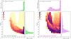 |
Fig. B.1. Heat map showing the probability distribution of period (P) and mass ratio (q) from our LMC synthetic population of CBs and near-CBs, tailored for the OGLE sample. The SMC has a closely similar P − q distribution as the LMC for massive CBs, as determined in Paper I. |
Small Magellanic Cloud massive contact binary candidates from the OGLE survey.
All Tables
Large Magellanic Cloud massive contact binary candidates from the OGLE survey.
Small Magellanic Cloud massive contact binary candidates from the OGLE survey.
All Figures
|
Fig. 1. OB binaries with periods P ≤ 3 days across all morph parameter values (from 0 to 1), identified as MS systems from the OGLE sample (light grey dots) on the absolute color (MV, max − MI, max) – magnitude (MV, max) space (where, the absolute magnitudes correspond to their values at maximum brightness of the binary). Overlaid are the empirically identified OGLE EW+ subsample from the LMC (yellow circles, as described in Section 2.2). Curves indicate the limits of the ZAMS and TAMS curves computed from non-rotating and rotating (vi = 330 km/s) models of single stars with masses of 7 − 50 M⊙. |
| In the text | |
|
Fig. 2. Characterization of the OGLE binary sample. The black filled circles represent the ratio of LMC to SMC OGLE binaries, red circles are the same ratio but for Gaia MS stars, and blue triangles are the percentage binary fractions (OGLE/Gaia) for the LMC (filled triangles) and SMC (open triangles). The x-axis represents the absolute V-band magnitude MV (or MV, max in the case of OGLE binaries). Error bars represent Poisson uncertainties |
| In the text | |
|
Fig. 3. Exemplary I-band light curves from the OGLE database, classified by this study as EW (top), EB (middle) and ELL (bottom). The OGLE database itself uses a different classification scheme. |
| In the text | |
|
Fig. 4. Panels showing the evolution of the exemplary ‘System 2’ binary model from Paper I, with initial parameters: MT, i = 26 M⊙, Pi = 1.0 d, and qi = 0.8. The parameters from top to bottom panels are: the fill-out factor (R/RRL), the temperature and mass ratio (T2/T1; q), orbital period (P), mass of both components and the mass-transfer rate. Also shown are the contact (light-green region) phase and near-contact (pink region) phase, which is further divided into the detached phase (crosshatching) and semi-detached phase (striped hatching). The open circles are the instances at which synthetic PHOEBE light curves are computed (Fig. 5). |
| In the text | |
|
Fig. 5. Light curves computed for System 2 at the various evolutionary points marked in Fig. 4, at inclinations of i = 30°, 60° and 90°. Top panel: Light curves from the contact phase (green region in Fig. 4), where the cyan light curve represents the dominant type of CB expected from models, i.e., one which has acquired temperature equalization. Bottom panel: Light curves during the near-contact phase CB (pink striped region in Fig. 4), which is further split as a semi-detached (red and orange light curves) and detached system (cyan light curve). Also labeled are the relative eclipse depths, fΔA, except for ELL binaries, which have an fΔA of the order of 0.001. |
| In the text | |
|
Fig. 6. Heat map showing the probabilistic distribution of the absolute color (MV, max − MI, max) and magnitude (MV, max) at the maximum brightness (i.e., the sum of intrinsic luminosities of both components) of CBs for the LMC and SMC. The OGLE data are marked as follows: OGLE bona fide CB sample (blue diamonds), OGLE EW+ subsample (yellow circles) and OGLE Rest (grey dots), which is the sample with morph parameter c > 0.7 and P ≤ 3 days that did not make the cut into either the EW+ nor the bona fide CB sample. For reference, the theoretical ZAMS and TAMS curves from Fig. 1 are also marked. |
| In the text | |
|
Fig. 7. Heat map showing the probabilistic distribution of the absolute magnitude (MV, max) at maximum brightness to orbital period (P) of CBs, for the LMC and SMC. O- and B-type systems are distinguished by a magnitude cutoff at MV, max = −4. The OGLE data are annotated as in Fig. 6. For reference, the theoretical extent of the bona fide CB sample is indicated by the polygon outlined in blue dots, beyond which their number counts from de-convoluted histograms (green histograms) drop below one. |
| In the text | |
|
Fig. B.1. Heat map showing the probability distribution of period (P) and mass ratio (q) from our LMC synthetic population of CBs and near-CBs, tailored for the OGLE sample. The SMC has a closely similar P − q distribution as the LMC for massive CBs, as determined in Paper I. |
| In the text | |
Current usage metrics show cumulative count of Article Views (full-text article views including HTML views, PDF and ePub downloads, according to the available data) and Abstracts Views on Vision4Press platform.
Data correspond to usage on the plateform after 2015. The current usage metrics is available 48-96 hours after online publication and is updated daily on week days.
Initial download of the metrics may take a while.