| Issue |
A&A
Volume 705, January 2026
|
|
|---|---|---|
| Article Number | A245 | |
| Number of page(s) | 18 | |
| Section | Planets, planetary systems, and small bodies | |
| DOI | https://doi.org/10.1051/0004-6361/202555433 | |
| Published online | 23 January 2026 | |
The coupled tidal evolution of the moons and spins of warm exoplanets
1
Department of Astrophysical Sciences, Princeton University,
4 Ivy Lane,
Princeton,
NJ
08540,
USA
2
Canadian Institute for Theoretical Astrophysics,
60 St. George Street,
Toronto,
ON
M5S 3H8,
Canada
3
LTE, Observatoire de Paris, Université PSL, Sorbonne Université, Université de Lille, LNE, CNRS,
61 Avenue de l’Observatoire,
75014
Paris,
France
★ Corresponding authors: This email address is being protected from spambots. You need JavaScript enabled to view it.
; This email address is being protected from spambots. You need JavaScript enabled to view it.
Received:
8
May
2025
Accepted:
31
October
2025
Abstract
Context. The Solar System giant planets harbor a wide variety of moons. Among them, the largest moons have moon-to-planet mass ratios of the order of 10−4. Moons around exoplanets are plausibly similarly abundant, even though most of them are likely too small to be easily detectable with modern instruments. Moons are known to affect the long-term dynamics of the spin of their host planets; however, their influence on warm exoplanets (i.e. with moderately short periods of about 10 to 200 days), which undergo significant star–planet tidal dissipation, is still unclear.
Aims. Here, we study the coupled dynamical evolution of exomoons and the spin dynamics of their host planets, focusing on warm exoplanets.
Methods. Analytical criteria give the relevant dynamical regimes at play as a function of the system’s parameters. Possible evolution tracks mostly depend on the hierarchy of timescales between the star–planet and the moon-planet tidal dissipations. We illustrate the variety of possible trajectories using self-consistent numerical simulations.
Results. We find two principal results: i) Due to star–planet tidal dissipation, a substantial fraction of warm exoplanets naturally evolve through a phase of instability for the moon’s orbit (the ‘Laplace plane’ instability). Many warm exoplanets may have lost their moon(s) through this process. ii) Surviving moons slowly migrate inwards due to the moon-planet tidal dissipation until they are disrupted below the Roche limit. During their last migration stage, moons – even small ones – eject planets from their tidal spin equilibrium. Planets can then converge back to this equilibrium or adopt a new one with a low or high obliquity. Additionally, before their disruption, massive exomoons (with moon-to-planet mass ratios of the order of 10−2) can maintain their planet in a long-lived high-obliquity state.
Conclusions. The loss of moons through the Laplace plane instability may contribute to disfavor the detection of moons around close-in exoplanets. Moreover, moons (even those that have been lost) play a critical role in the final obliquities of warm exoplanets. Hence, the existence of exomoons poses a serious challenge in predicting the present-day obliquities of observed exoplanets.
Key words: planets and satellites: dynamical evolution and stability
© The Authors 2026
 Open Access article, published by EDP Sciences, under the terms of the Creative Commons Attribution License (https://creativecommons.org/licenses/by/4.0), which permits unrestricted use, distribution, and reproduction in any medium, provided the original work is properly cited.
This article is published in open access under the Subscribe to Open model. This email address is being protected from spambots. You need JavaScript enabled to view it. to support open access publication.
1 Introduction
The obliquity of a planet, the angle between its spin and orbital axes, is affected by a number of processes. In the Solar System, the planets’ obliquities range from nearly zero for Mercury to about 180◦ for Venus, including the puzzling 98◦ value of Uranus. This large variety of obliquities is likely the result of distinct combinations of dissipative processes, giant impacts, as well as spin–orbit and precession resonances (e.g., Goldreich & Peale 1966; Safronov 1966; Gold & Soter 1969; Tremaine 1991; Laskar & Robutel 1993; Touma & Wisdom 1993; Correia & Laskar 2001; Ward & Hamilton 2004; Hamilton & Ward 2004; Ward & Canup 2006; Boué & Laskar 2010; Vokrouhlický & Nesvorný 2015; Rogoszinski & Hamilton 2020, 2021).
Recently, the first constraints on the obliquities of exoplanets have become possible (Bryan et al. 2020, 2021; Palma-Bifani et al. 2023; Poon et al. 2024). Such measurements have become significantly more feasible with the launch of the James Webb Space Telescope, which can help infer a planet’s spin state via either asymmetries in its transit light curve (for giant planets; Lammers & Winn 2024; Liu et al. 2025; Lu et al. 2025) or direct measurement of its thermal phase curve (for close-in planets; Greene et al. 2023; Hu et al. 2024; Hammond et al. 2024). The obliquities of exoplanets are important because they are strong markers of the formation processes and subsequent dynamical evolution of planets, as witnessed by the Solar System planets (Levrard et al. 2007; Fabrycky et al. 2007; Millholland & Laughlin 2018; Millholland & Laughlin 2019; Millholland & Spalding 2020; Su & Lai 2021). Moreover, planetary obliquities play a decisive role in the dynamics – and possible detection – of moons and rings around exoplanets (see Ohta et al. 2009; Tremaine et al. 2009). Because of the close connection between the obliquity and climate of a planet, exoplanetary obliquities are also of critical importance for habitability studies (Kite et al. 2011; Ferreira et al. 2014; Penn & Vallis 2017; Lobo & Bordoni 2020; Guerrero et al. 2024).
Recent works suggest that the orbital migration of the moons of Jupiter, Saturn, and possibly Uranus are a key ingredient needed to explain the obliquities of these planets (Saillenfest et al. 2020, 2021a,b; Wisdom et al. 2022; Dbouk & Wisdom 2023), and Earth’s relatively much more massive moon also greatly affects its spin evolution (see e.g., Goldreich 1966; Laskar et al. 1993). This is in spite of the comparatively small masses of the moons, which tend to have moon-to-planet mass ratios ≲10−4. The dynamical effect that makes this possible is a secular spin–orbit resonance, a commensurability between the precession of the planet’s spin axis about its orbit normal (modulated by the moon) and a harmonic of the precession of the planet’s orbit about the planetary system’s invariable plane (e.g., Colombo 1966; Peale 1969; Boué & Laskar 2006; Saillenfest et al. 2019, 2021a). While exomoons with such small masses are likely undetectable with present-day instruments, the ongoing interest in exomoon detection (e.g., Kipping 2009; Teachey & Kipping 2018; Kipping et al. 2022; Yahalomi et al. 2024) as well as their aforementioned significant effect on planetary obliquities motivate careful study of their dynamical impact.
While the general problem of predicting exoplanetary obliq-uities requires understanding both planet formation and subsequent dynamical evolution (e.g., Dones & Tremaine 1993; Millholland & Batygin 2019; Su & Lai 2020; Li et al. 2021), and it generally yields a wide range of possible final states, the obliquities of warm exoplanets are in theory able to be much better forecast. Indeed, the star–planet tidal dissipation generally drives the planet’s obliquity to zero in the absence of secular spin–orbit resonances, or to one specific state among a few stable equilibria in the presence of resonances (Ward 1975; Levrard et al. 2007; Fabrycky et al. 2007; Saillenfest et al. 2019; Su & Lai 2021; Su & Lai 2022). The precise outcome of resonance encounter and capture can be modeled as a probabilistic event and be efficiently quantified (Henrard 1982; Henrard & Murigande 1987; Henrard 1993; Su & Lai 2021). However, many exoplanets probably have (or have had) moons that continuously migrate as a result of tidal dissipation. The effect of exomoons on previous predictions of the obliquity states of warm planets has not been previously considered.
In this work, we aim to determine the possible spin history of planets subject to: (i) orbital perturbations from other planets, (ii) a dissipative torque from its host star, and (iii) an additional torque from a moon that may migrate inwards or outward due to moon-planet tidal dissipation. These basic ingredients are generic for close-in planets and expected to be very common in exoplanetary systems. According to the actual hierarchy of timescales between each dynamical effect, a rich variety of evolutions can be produced, and we investigate a few of interest here. Note that we restrict our attention to the constant time lag model (Alexander 1973; Hut 1981) of tidal dissipation: the internal structures of exoplanets are poorly known, and even less is known about their tidal dissipation properties. Therefore, in this first attempt to explore the coupled dynamics of close-in planets and their exomoons, we do not try to cover the wealth of possible evolution pathways that could be produced by different tidal models, particular rheologies, and dynamical interiors (see e.g., Ferraz-Mello 2013; Boué et al. 2016; Fuller et al. 2016; Ragazzo & Ruiz 2017; Ferraz-Mello et al. 2020; Boué 2020).
In Sect. 2, we recall the dynamical mechanisms at play and outline the basic equations that govern the spin, orbit, lunar, and tidal evolutions. We then describe trajectories obtained in three different regimes according to the ratio between the timescale of star–planet tidal dissipation τp and that of moon-planet tidal dissipation τm. In Sect. 3, we first study the regime where τm ≲ τp and find that the planet spindown enhances obliquity excitation due to lunar migration. This section connects our work to previous studies which have focused on the regime τm ≪ τp. In Sect. 4, we study the early phases of the regime where τm ≫ ωp and show that moons can be lost more frequently than previously thought. In Sect. 5, we study the late phases of the same regime τm ≫ ωp, where the eventual runaway tidal inspiral of the moon breaks the planet out of its tidal equilibrium state. We summarize and discuss our results in Sect. 6.
2 Theoretical background
In this section, we describe some simple, and sometimes approximate, analytical results that are useful toward understanding the combined spin and orbital evolution of planets and their moons. Later in this paper, we use these results to analyze numerical simulations that are not subject to the same approximations.
2.1 Spin-orbit precession and secular resonances
In this section, we follow the formalism of Saillenfest et al. (2019) and Su & Lai (2021), with some changes in notation. We consider a star hosting several planets that perturb each other’s orbits. We study the spin dynamics of one of these planets denoted with the subscript “p” (to distinguish quantities related to the planet from quantities related to its moon, see below). We assume that the planetary system is long-term stable, then the orbital inclination of the planet can be written (at least locally in time) as a convergent quasi-periodic series truncated to N terms:
![Mathematical equation: ${\zeta _{\rm{p}}} \equiv \sin {{{I_{\rm{p}}}} \over 2}\exp \left( {i{\Omega _{\rm{p}}}} \right) = \sum\limits_{j = 1}^N {{\Upsilon _j}} \exp \left[ {i{\phi _j}(t)} \right]$](/articles/aa/full_html/2026/01/aa55433-25/aa55433-25-eq1.png) (1)
(1)
Here, Ip is the orbital inclination of the planet and Ωp is its longitude of ascending node measured in some inertial reference frame. Υj is a real positive constant and  evolves linearly with time t with frequency νj. Such a quasi-periodic decomposition can be obtained from an analytical theory (e.g. the Lagrange–Laplace system, see Murray & Dermott 1999) or from a Fourier analysis of a numerical solution (see e.g. Laskar 1988, 1990). Equation (1) defines the motion of the unitary orbital angular momentum vector Îp of the planet due to interactions with the other planets in the system via
 (2)
(2)
Next, we study the evolution of the unitary spin angular momentum of the planet, denoted ŝp. In the absence of moons, the dominant torque on ŝp is due to the attraction of the star on the planet’s equatorial bulge. At quadrupolar order, and upon averaging over the fast orbital and spin angles, the equation of motion for ŝp is
 (3)
(3)
where
 (4)
(4)
(see e.g., Laskar & Robutel 1993, Eq. (2)). Here, 𝒢 is the gravitational constant, m⋆ is the mass of the star, ap and ep are the semi-major axis and eccentricity of the planet’s orbit around the star, J2 is the second zonal gravity coefficient of the planet, ω is its spin rate, and λ is its normalized polar moment of inertia. The quantities J2 and λ are defined using the same normalising radius Rp of the planet (e.g. its equatorial radius at time t = 0).
In Eq. (3), the spin-axis motion of the planet is forced by its orbital motion through the explicit time dependence of Îp coming from Eq. (1). As the orbital angular momentum of the planet is much larger that its spin angular momentum, the back reaction of the planet’s spin-axis motion on the planet’s orbit is negligible.
The obliquity θ of the planet is defined as cos θ = ŝp · Îp. Because of the motion of the planet’s orbital plane, the planet’s spin-axis dynamics is affected by secular spin–orbit resonances, that is, by resonances between the precession of the spin axis and one or several harmonics appearing in Eq. (1). As detailed by Saillenfest et al. (2019), the strongest resonances are of order 1 in the amplitudes Υj. If the planet is trapped in such a resonance with harmonic j = k, then the resonance angle σ = ψ + ϕk oscillates around a fixed value, where ψ is the precession angle of the planet’s spin axis (following the convention of Laskar & Robutel 1993; Saillenfest et al. 2019). In other words, the planet’s obliquity θ evolves such that the relation α cos θ + νk ≈ 0 is maintained. This kind of equilibrium is called a ‘Cassini State’ (see e.g. Peale 1969; Henrard & Murigande 1987). Depending on the value of parameters, there can be up to four distinct Cassini states.
Neglecting terms of order  and beyond, we introduce the nondimensional variables γ = fγ/α and β = fβ/α, where
 (5)
(5)
As an immediate property of the Lagrange–Laplace system, we expect dominant terms in Eq. (1) to have negative frequencies νj if the planetary system is roughly coplanar (see e.g., Laskar 1990). This means that for the strongest resonances, γ and β are both positive.
At the vicinity of resonance with harmonic k, Eq. (3) can be rewritten component-wise as (see Saillenfest et al. 2019, Eq. (16))1
 (6)
(6)
 (7)
(7)
The Cassini states are the equilibrium points of this system of two equations. For γ2/3 + β2/3 ⩾ 1, there are only two distinct Cassini states and no resonance can be defined (i.e. there is no separatrix). For γ2/3 + β2/3 < 1, there are four Cassini states, and a separatrix encloses the resonance region. The equilibrium points corresponding to the resonance centeris called ‘Cassini state 2’.
If the orbital inclination dynamics of the planet is dominated by one single harmonic in Eq. (1) with frequency ν and amplitude Υ = sin(Ip/2), then, only one secular spin–orbit resonance exists. For this isolated resonance, γ and β are simplified to γ = −ν cos Ip/α and β = −ν sin Ip/α, and we recover the for-mulas given by Su & Lai (2021). In general, however, the orbital dynamics of planets are composed of many harmonics that create a web of resonances. These resonances can either be isolated (see e.g. Saillenfest et al. 2020) or overlap and create chaotic zones (see Laskar & Robutel 1993).
2.2 Tidal dissipation and stable equilibria
We consider that the planet is relatively close to its host star, with an orbital period smaller than a few hundred days. In this case, the substantial star–planet tidal interactions produce redistributions of mass inside the planet, leading to a dissipation of energy. Using the standard ‘constant time lag’ weak friction theory of the equilibrium tide (Alexander 1973; Hut 1981; Lai 2012), the spin rate ω and obliquity θ of the planet evolve due to tidal dissipation, following
![Mathematical equation: ${\left. {{{{\rm{d}}\omega } \over {{\rm{d}}t}}} \right|_{{\rm{tides }}}} = {\omega \over {{\tau _{\rm{p}}}}}\left[ {{{2{n_{\rm{p}}}} \over \omega }\cos \theta - \left( {1 + {{\cos }^2}\theta } \right)} \right],$](/articles/aa/full_html/2026/01/aa55433-25/aa55433-25-eq10.png) (8)
(8)
 (9)
(9)
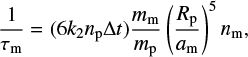
where np is the mean motion of the planet, and τp is the tidal timescale. Assuming that the planet behaves as a self-gravitating fluid, τp is given by
 (10)
(10)
where ∆t is the tidal time lag2 and k2 is the second tidal Love number of the planet. Due to planetesimal accretion for small planets (Dones & Tremaine 1993; Miguel & Brunini 2010), and to a combination of runaway accretion and magnetic despinning for giant planets (Takata & Stevenson 1996; Batygin 2018), we can expect planets to be born with a spin rate up to critical rotation. Therefore, their initial spin rates ω0 can be substantially supersynchronous:
 (11)
(11)
where  is the critical spin rate of the planet above which its centrifugal potential overwhelms its gravitational potential. As a consequence, the time it takes for a planet to become tidally synchronized (i.e. to reach ω ≈ np) is typically several τp.
As ω evolves due to tidal dissipation, the planet’s oblateness evolves following its hydrostatic equilibrium figure (Eggleton 2006),
 (12)
(12)
where k2 is the hydrostatic Love number of the planet.
The variations in ω mean that the coefficient α in Eq. (4) is not constant; yet, the change in α due to tidal dissipation is considered to be slow enough so that Eqs. (6) and (7) still hold, with α treated as a slowly-varying parameter. Hence, the complete set of equations that governs the spin-axis dynamics of the planet due to secular spin–orbit resonances and star–planet tidal dissipation is obtained by adding both contributions (see Eqs. (6)–(7) and (8)–(9)), resulting in a system of three equations for the variables (ω, θ, σ).
The equilibria of this system are the ‘tidal Cassini equilibria’ (or tCE; see Su & Lai 2021). In the limit of weak dissipation, the locations of tCE only depend on γsync = fγ/αsync and βsync = fβ/αsync, where αsync is the value of α computed at ω = np. For a configuration of the system to be a tCE, Eq. (8) implies that the planet must have reached the pseudo-synchronous spin state, that is,
 (13)
(13)
This condition requires the planet’s spin at equilibrium to be prograde, that is, θ ⩽ 90◦. For  , there is only one tCE, called tCE2, which corresponds to the Cassini state 2 at pseudo-synchronisation3. For
  , there are two tCE, called tCE1 and tCE2, which correspond to the Cassini states 1 and 2 at pseudo-synchronisation. The one with higher obliquity is tCE2; it is located at the centerof the secular spin– orbit resonance. In order for the Cassini states 1 and 2 to exist at θ ⩽ 90◦, the frequency νk of the resonance needs to be negative, which implies that γ and β are positive.
In the limit α ≫ |νk|, that is, γ ≪ 1 and β ≪ 1, the Cassini state 2 is located at cos θ ≈ γ. By virtue of (13), the obliquity and spin rate at tCE2 are therefore
 (14)
(14)
 (15)
(15)
2.3 Tidal resonance breaking
For strong enough dissipation (i.e. small enough tidal timescale τp), the high-obliquity Cassini state 2 is no longer stable to tidal dissipation (specifically, it undergoes a saddle node bifurcation with the unstable Cassini State 4 Levrard et al. 2007; Fabrycky et al. 2007; Su & Lai 2021). Indeed, Eqs. (6) and (9) imply that a necessary condition for dθ/dt to have a zero is
 (16)
(16)
Evaluating this equation for ω and θ given by Eqs. (14) and (15), we obtain that
 (17)
(17)
This is a necessary condition for tCE2 to be stable to tidal dissipation. As such, if the tidal timescale τp becomes sufficiently short, or if γsync becomes sufficiently small, then the planet is ejected out of the high-obliquity tCE2, whereupon it settles into the low-obliquity tCE1.
2.4 Precession dynamics with a moon: general theory
We next consider the spin dynamics of the planet as affected by a moon in orbit around it. Since the moon’s eccentricity is expected to damp relatively rapidly (e.g. Goldreich & Gold 1963), we consider for now that the moon’s orbit is circular. Otherwise, call the moon’s mass mm, its semimajor axis am, and the inclination of its orbit relative to the planet’s equatorial plane im.
The orbit of a moon is affected by secular precessional torques from both the planet’s equatorial bulge and the distant host star. In the limit of a massless moon, there are six equilibria of these precession equations, known as the Laplace states (Tremaine et al. 2009; Saillenfest & Lari 2021). We note them P1, P2, P3, and P−1, P−2, P−3, where the negative indexes denote the twin equilibria under the transformation Îm → −Îm, where Îm is the moon’s orbit normal. Since regular moons probably form in an environment where damping is efficient due to gas drag and/or mutual collisions, their initial orbital plane is thought to lie very close to a stable equilibrium near the equator of their host planets. The Laplace states corresponding to such an equilibrium are P1 and P−1, which are denoted the “circular coplanar Laplace equilibrium” by Tremaine et al. (2009). In the limit of a massless moon, the inclination of P1 is given by (Saillenfest & Lari 2021; see Boué & Laskar 2006 for the general expression)
![Mathematical equation: ${i_{{\rm{m}}1}} = {1 \over 2}\left[ {\pi + {\mathop{\rm atan}\nolimits} 2\left( { - \sin 2\theta , - {{\left( {{r_{\rm{M}}}/{a_{\rm{m}}}} \right)}^5} - \cos (2\theta )} \right)} \right],$](/articles/aa/full_html/2026/01/aa55433-25/aa55433-25-eq23.png) (18)
(18)
where
 (19)
(19)
is the “midpoint radius”, related to the canonical Laplace radius rL (Tremaine et al. 2009) via  . We prefer to use rM since it is the lunar semimajor axis at which im1 lies exactly halfway between the planet’s equatorial and orbital planes (i.e., im1 = θ/2 for θ < 90◦). For clarity, we call im,−1 the inclination of P−1 (i.e., the “twin” state to P1 with reversed lunar orbital motion). Its value is
 (20)
(20)
The behavior of im1 as functions of the evolving system parameters is illustrated in Fig. 1. Depending on the formation process of regular moons (e.g., in a primordial circumplanetary disk, or as a second generation moon system following a tilting impact; see e.g. Morbidelli et al. 2012), their orbits can be initially prograde or retrograde to their planet’s spin. If we consider a pro-grade moon around a retrograde spinning planet (i.e., θ > 90◦, such as the major moons of Uranus), this moon occupies the P−1 state and has an inclination equal to im,−1. Following Fig. 1, we see that such a moon evolves into a retrograde orbit by the time the planet has despun (left panel in conjunction with Eq. (20); see also Figs. 3 and 4 in Saillenfest & Lari 2021). This is because the oscillations of the moon’s orbital pole around the stable equilibrium occur on a much shorter timescale than the despinning of the planet, such that the moon adiabatically follows the equilibrium.
For a moon located in the P1 or P−1 state, the spin-axis precession of the planet is modified by replacing α in Eq. (3) by
 (21)
(21)
where we define the effective J2 and λ as (French et al. 1993; Boué & Laskar 2006; Saillenfest & Lari 2021)
 (22)
(22)
 (23)
(23)
and im is equal to either im1 or im,−1. Here, nm is the moon’s mean motion. We note that this expression differs from that used by Ward & Hamilton (2004) and Millholland & Laughlin (2019) – see discussion by Saillenfest & Lari (2021)4. For tidally despun planets, we stress that both λ′ and  generally differ substantially from λ and J2.
As first pointed out by Tremaine et al. (2009), the P1 and P−1 state of the moon are linearly unstable to eccentricity growth in a closed region of the space (am/rM, θ). We call this region E1; it has a cardioid-like shape, whose border has a simple analytical expression (see Saillenfest & Lari 2021 and the hatched region in Fig. 1). Qualitatively, the E1 region lies at am ∼ rM for planet’s obliquity values θ ∈ [68.9◦, 111.1◦]. When smoothly entering E1 via a slow change of parameters, trajectories on the circular P1 and P−1 equilibria transition to stable eccentric equilibria, which then become linearly unstable deeper in the E1 region.
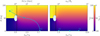 |
Fig. 1 Orbital inclinations of Laplace state P1 and its twin P−1 (colorbar, given by Eqs. (18), (20)) as functions of am/rM and the planet’s obliquity θ. In both panels, the location of am = rM is denoted with a vertical black dashed line, and the E1 region (where P1 and P−1 are unstable) is shown by a white hatched zone. Across the two panels, a representative evolutionary history is shown via the three cyan points and arrows (S1, S2, S3). While the inclinations of P1 and P−1 only depend on θ and am/rM, we also illustrate the evolution using the following concrete parameters for interpretability: ap = 0.4 au, ep = 0, Rp = 2 R⊕, and mp = 10 M⊕. We then denote the corresponding values of the planet’s spin rate along the top-left axis (relevant to planetary tidal evolution) and the lunar semi-major axis along the top-right axis (relevant to lunar migration). In the left panel, the planet is initially rapidly rotating with a period of 7.5 hours, and the moon is located at am = 5Rp (S1). Then, as the planet despins and the obliquity damps, rM decreases while the moon is still located at am = 5Rp, and the system reaches S2 (we have neglected lunar tidal migration for illustrative purposes). Going from S1 to S2, the inclination of the lunar orbit smoothly flips from prograde to retrograde (assuming that the moon occupies P−1). In the right panel, as the moon inspirals, starting from S2, am decreases until the moon is disrupted by the planet when am ≃ Rp ≳ rM (S3). |
2.5 Precession dynamics with a moon: synchronously spinning planet
Here, we derive some special cases of the results presented in the previous section for applications toward planets that have tidally synchronized. First, for ep = 0 and mp ≪ m⋆, the midpoint radius rM can be approximated by
 (24)
(24)
As such, we can see that as planets approach spin–orbit synchronization, rM ≲ Rp, so their moons are always exterior to the midpoint radius (by merit of being outside of the planet).
Next, we seek expressions for α′ in this limit. It follows from Eqs. (18) and (19) that when am ≫ rM,
 (25)
(25)
![Mathematical equation: ${\alpha ^\prime } \approx {\alpha _0}\left[ {1 + {{{m_{\rm{m}}}a_{\rm{p}}^3} \over {{m_ \star }a_{\rm{m}}^3}}} \right]{{{\lambda ^\prime }} \over \lambda }.$](/articles/aa/full_html/2026/01/aa55433-25/aa55433-25-eq33.png) (26)
(26)
Since λ ≫ J2, the relative change from λ to λ′ is often modest, even while the relative change from J2 to  is significant (Eqs. (22) and (23)). Accordingly, α′ only varies moderately as the planet spins down, and it is constant in the limit λ′ ≈ λ.
2.6 Lunar orbit evolution
Throughout this paper, we consider cases for which the planet’s spin evolution due to the tide raised by the star is either slower or faster than the moon’s orbital evolution due to the tide it raises on the planet. The variety of possible evolution pathways depend on the hierarchy between these two timescales. By looking at the major moons in the Solar System, we know that regular moons can be found at distances am between a few and a few tens of Rp. The most distant major moons may have reached their current distances through tidal migration (see e.g., Goldreich & Soter 1966; Lainey et al. 2020). Adopting the same constant time lag model as in Sect. 2.2, but for the lunar tide, the lunar orbit evolves following:
 (27)
(27)
 (28)
(28)
 (29)
(29)
The backreaction of the moon’s orbital evolution on the planet’s spin tends to drive the planet toward synchronization and alignment with the orbit of its moon on characteristic timescale
 (30)
(30)
For the fiducial values considered in Eq. (29), the lunar tide typically results in evolution on longer timescales than the stellar tide (i.e., τp,m > τp). However, for more sophisticated tidal processes, lunar inspiral can be accelerated compared to the naïve model considered here. For instance, resonance locks are thought to be responsible for the anomalously rapid migration of the moons of Saturn (Fuller et al. 2016; Lainey et al. 2020; but see also Jacobson 2022). We note here that we also neglect the effect of cross tides, a phenomenon that arises when two bodies raise tidal perturbations on the same primary (Goldreich 1966; Touma & Wisdom 1994; Neron de Surgy & Laskar 1997). We justify this omission in Appendix A.
2.7 Numerical procedure
The previous subsections outline the dominant effects at play, allowing us to get an intuition of the possible evolutionary tracks of the planet and its moon. For the case studies analyzed in the following sections, we systematically validate our analytical approximations and explore the dynamics in more details using a self-consistent numerical model.
Our numerical experiments below are produced with the coupled equations of motion of the planet’s spin axis and the orbit of its moon. The methodology is described in Appendix C of Saillenfest et al. (2022): It is based on the secular equations of motion expanded to quadrupole order developed by Correia et al. (2011), which are valid for arbitrary eccentricities and inclinations for the planet and the moon. The orbital evolution of the moon is integrated self consistently, with no assumption regarding its eccentricity or inclination. In order to reproduce the perturbations from additional planets in the system, the orbital evolution of the planet is made to vary with quasi-periodic series as in Eq. (1).
The tidal dissipation due to the stellar torque acting on the planet’s spin axis is included using the constant time lag theory (see Sect. 2.2 and Eq. (22) of Correia et al. 2011). As the orbital angular momentum of the planet is much larger than its spin angular momentum, we neglect any dissipative effect on the planet’s orbit (i.e., the planet does not migrate on its orbit around the star).
Depending on the section, the tidal dissipation due to the moon’s torque is included in a different way. In Sect. 3, the moon’s orbital migration (i.e., the evolution of its semi-major axis) is introduced as a pre-defined function of time, and we neglect its effect on the planet’s despinning. In Sects. 4 and 5, the moon’s migration and tidal despinning of the planet are included self consistently: the moon migrates as a response of angular momentum transfer (see Eq. (20) of Correia et al. 2011). Each setting is described in the corresponding section.
As the equations of motion are averaged over the mean anomaly of the moon and the mean anomaly of the planet, nonsecular effects such as evection and eviction-like resonances are not included in our numerical experiments (see Touma & Wisdom 1998; Vaillant & Correia 2022). This choice is justified in Appendix B. We show that evection and eviction-like resonances do not play a role here because the star–planet tidal dissipation despins the planet to near spin–orbit synchronization; As a consequence, these resonances are shifted to distances below the planet’s own radius before the moon has a chance to reach them.
Our numerical experiments do not include tidal dissipation within the moon’s interior or the evolution of the moon’s spin axis. The moon is always treated here as a point mass. This approximation is justified by the timescales at play. As the moon adiabatically follows its Laplace plane equilibrium, its orbital eccentricity remains small at all times (this is verified in all simulations). The only substantial eccentricity increase of the moon is due to crossing the unstable E1 region. The timescale of exponential eccentricity increase in the E1 region is given by Eq. (19) of Saillenfest & Lari (2021), adapted from Tremaine et al. (2009). Once inside the E1 region, the timescale for the moon’s eccentricity to be multiplied by 100 drops rapidly below hundreds of years for all physical parameters considered here (see also Fig.7 by Saillenfest et al. 2022 for a distant Uranus-like planet). This very short timescale should be compared to the eccentricity damping timescale due to tidal dissipation within the moon. Using classical formulas (e.g., Eq. (4.198) by Murray & Dermott 1999) with physical parameters consistent with those of the moons considered in this paper, we invariably obtain timescales that count in millions of years. Due to the many orders of magnitude different between these two timescales, we conclude that tidal dissipation within the moon would not qualitatively change the picture here. The same argument applies to obliquity tides: as the moon adiabatically follows its Laplace plane equilibrium, its spin axis would adiabatically follow its orbit normal. The moon may acquire a substantial nonzero obliquity only in the E1 region, but there the destabilization timescale is so fast that obliquity tides would not have time to operate.
3 Slow planet spindown: Generating long-lived high-obliquity planets
We first consider the case τp ≳ τm. Saillenfest & Lari (2021) have shown how the tidal migration of a moon can lead to a capture of the host planet in secular spin–orbit resonance. As the moon continues migrating, the planet’s obliquity increases and the system converges toward the unstable region E1. This phenomenon has been shown to be efficient for distant planets such as Jupiter, Saturn, and Uranus, for which the star-driven tidal despinning is negligible (i.e. τp ≫ τm). It may also be responsible for the formation of a very oblique ring around the long-period exoplanet HIP 41378 f (Saillenfest et al. 2023). The question then naturally arises about how this mechanism is modified for closer-in planets, for which the star–planet tidal dissipation is nonnegligible (i.e., τp ≳ τm). We illustrate this regime with numerical experiments using the code described in Sect. 2.7.
The interior structure of the planet is unknown, and the presence of resonances with internal oscillations modes can greatly enhance or decrease tidal dissipation (see e.g., Fuller et al. 2016; Farhat et al. 2022); for this reason, the details of the moon migration law are essentially unconstrained. Therefore, in this section we set the outward orbital migration of the moon as a predefined function of time (e.g., a linear law) and we neglect its corresponding contribution to the despinning of the planet (i.e., we consider that τp,m = ∞). This approximation is relevant for small moons around rapidly rotating planets – for which the moon orbital angular momentum is negligible compared to the spin angular momentum of the planet. The validity of this approximation is verified a posteriori: including the moon-driven tidal dissipation does not noticeably affect the trajectories shown in this section. The moon is initialized with 10−4 seed eccentricity and an inclination of 10−4 rad with respect to its local Laplace plane.
The red curve in Fig. 2 shows the obliquity evolution of the exoplanet HIP 41378 f as a result of the outward tidal migration of a hypothetical moon. Once the system reaches the unstable region E1, the moon’s eccentricity increases very rapidly, until the moons is disrupted below the planet’s Roche limit. The planet’s obliquity then becomes extremely stable, away from any resonance (see Saillenfest et al. 2023). In order to power the moon migration, the tidal time lag of the planet is assumed here to be of the order of ∆t = 3 × 10⁻⁹ yr, which is the value measured for Io and Jupiter5 (Lainey et al. 2009). HIP 41378 f being distant from its host star (period 541 days; semi-major axis 1.41 au), the inclusion of the star–planet tidal dissipation with this value of ∆t does not noticeably affect the dynamics. In other words, τp ≫ τm, so the red trajectory in Fig. 2 is identical to that of Saillenfest et al. (2023), Fig. 4.
If we artificially increase the star–planet tidal dissipation, however, the dynamics of HIP 41378 f appreciably changes. The blue curve in Fig. 2 shows the evolution when using ∆t = 2 × 10⁻⁴ years, which mimics the tidal dissipation felt by a closer-in planet with orbital period 35 days (i.e., semi-major axis 0.23 au). Interestingly, resonance capture and obliquity increase still occur, but in a shorter time span. This is mostly due to the gradual spin down of the planet, which decreases its oblateness (see Eq. (12)). The planet’s spin down consequently decreases the critical distance rM that the moon must reach in order to fully tilt the planet through the resonance (see Eq. (24)). The tilting mechanism considered by Saillenfest et al. (2023) is therefore not hampered by star–planet tidal dissipation; it is accelerated. After the disruption of the moon, the planet’s obliquity is damped by tidal dissipation, as expected, and the planet converges toward spin–orbit synchronisation and zero obliquity. However, as the planet’s obliquity is very large just after the loss of the moon, the effect of tidal dissipation is minimized (see Eqs. (8) and (9)). Hence, for a moderately close-in planet with τp ≳ τm, as in the case shown by the blue curve, the damping process takes tens of billions of years, such that in practice, the planet keeps a large obliquity during the remaining lifetime of the planetary system.
For an even closer-in planet, the resonance capture and obliquity increase due to the moon is only limited to a small transient stage of the evolution (see black curve in Fig. 2, which mimics a planet with orbital period 10 days, i.e., semi-major axis 0.1 au). In that case, we have now τp < τm. The star–planet tidal dissipation is so strong that the obliquity is rapidly damped after the moon’s disruption. The same outcome would have been obtained if the planet had had no moon in the first place and had experienced no obliquity increase. Yet, it is interesting to note that even in the case of a strong dissipation, the resonance capture and obliquity increase still occurs, even though the moon has not much time to migrate at all before the planet has completely spun down. This shows that the star–planet tidal dissipation alone can reproduce the mechanism described by Saillenfest et al. (2023), even for a non-migrating moon. This property is illustrated by the green curve in Fig. 2, for which the moon migration is artificially turned off (i.e. τm = ∞). In this example, the resonance capture and obliquity increase is still due to the presence of the moon; however, the increase in am/rM is not due to an increase in am, but to a decrease in rM as a result of the planet’s spin-down. This is yet another way of showing that star–planet tidal dissipation assists the moon-induced tilting of the planet described by Saillenfest et al. (2023).
Previous articles showed how the geometry of resonances depends on the distance am of the moon (see e.g., Saillenfest & Lari 2021; Saillenfest et al. 2023). If instead, we assume that the moon does not migrate (i.e., am is fixed), but that the planet’s spin rate ω varies as a result of star–planet tidal dissipation, the properties of secular spin–orbit resonances can again be expressed as a function of only two variables: ω and θ. Figure 3 illustrates the result obtained for HIP 41378 f assuming different parameters for the moon. Interesting geometries can be observed. Even though the boost α′/α in the planet’s spin-axis precession rate due to the moon varies slowly when am ≫ rM (see Sect. 2.5), resonances still converge toward a singular point with θ = 90◦ near am ≃ rM (the blue hatched region in Panels c and d). Geometries also depend on the distance am of the moon, taken here as a parameter. Strictly speaking, the geometries observed in Fig. 3 are therefore relevant when the timescale of the star-driven tidal dissipation is much shorter than the timescale of moon migration (i.e., τp ≪ τm): this regime is the focus of the next two sections.
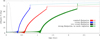 |
Fig. 2 Example of obliquity evolution of the planet HIP 41378 f and a hypothetical moon. The mass of the moon is m/M = 7 × 10⁻⁴, and it is initialized at a distance am = 5 Rp. For the red, blue, and black curves, the lunar migration rate is analogous to that measured for Io and Jupiter (Lainey et al. 2009). Dark colors show the trajectory when the moon is still present; light colors show the trajectory after the loss of the moon, assumed to be instantly disrupted once its pericenter goes below the Roche limit. For the red curve, the star–planet tidal dissipation is taken into account with tidal time-lag ∆t = 3×10⁻⁹ years. For the blue curve, the star–planet tidal dissipation is artificially increased using ∆t = 2×10⁻⁴ years. For the black curve, the star–planet tidal dissipation is artificially increased using ∆t = 2 × 10⁻² years. For the green curve, the moon’s migration is turned off, and the star–planet tidal dissipation is taken into account using ∆t = 2 × 10⁻⁴ years. |
4 Rapid planet spindown: Moon loss through the E1 instability
We next turn our attention to to the regime where the planet’s spindown is rapid, i.e. τp ≪ τm. In this regime, we identify a novel mechanism by which exoplanets can lose their moons as they spin down.
In previous studies, whether a moon can exist around a given planet is determined by whether the moon either experiences runaway tidal inspiral or tidally migrates beyond the stability limit am ≳ 0.36 rH (Barnes & O’Brien 2002; Sasaki et al. 2012; but see also Kisare & Fabrycky 2024), where rH is the planet’s Hill radius and is given by
 (31)
(31)
 (32)
(32)
Here, we show that moons need not reach the orbital stability limit to experience dynamical instability. The key to our mechanism is the dynamical instability of the P1 (or P−1) Laplace equilibrium when the system configuration is within the region E1. This can drive lunar instability at much smaller orbital separations than in previous works, since
 (33)
(33)
In order for the moon to experience this dynamical instability, the system must evolve through E1. There are two distinct tidal dissipation mechanisms that can contribute to such an evolution, which correspond to the limits τp ≪ τm and τp ≫ τm.
First, for τp ≪ τm, the tidal evolution of the young planet’s spin (predominantly driven by the host star) naturally acts to drive systems toward E1. As the planet spins down, its rM ∝ ω2/5 decreases (see Eq. (24)). Thus, since initially am < rM, the equality am = rM is satisfied at some point during the planet’s spindown. At the same time, tidal dissipation also drives the young planet’s obliquity toward 90◦ due to tidal dissipation when the planet’s spin is sufficiently rapid: to be precise, cos θ is driven toward 2np/ω ≪ 1, see Eq. (9)6. Combining these two observations, it is clear that evolution through E1 can be very common. We note that a passage through E1 leads to dynamical instability of the moon’s orbit on short timescales ( , which is much shorter than the tidal timescale τp; see Eq. (9) of Saillenfest & Lari 2021).
In Fig. 4, the lightly shaded regions denote the regions of parameter space such that the planet’s tidal evolution results in passage through E1; we have assumed that (i) the moon’s distance does not vary, and (ii) the moon adiabatically follows its Laplace state as the planet spins down. We consider two lunar distances, am = 5 Rp and 7 Rp, consistent with the locations of major regular moons in the Solar System. We note that for sufficiently small (θ ≈ 0◦) or large (θ ≈ 180◦) initial obliquities, the instability is not reached, but it is reached for a broad range of intermediate obliquities. This range is wider for planets that are born with larger ω/np, that is, for more distant planets that must despin more. However, the tidal timescale τp of more distant planets is larger, and possibly comparable with the moon migration timescale τm, which leads us to the second case.
If instead τp ≫ τm, the system can still pass through the E1 region because of the tidal evolution of the lunar orbit alone. In this case, the lunar orbit widens (due to the tide it raises on the rapidly rotating planet) such that am approaches rM from below. Such an evolution results in E1 passage for an intermediate range of obliquities (denoted by the dashed curves in Fig. 4). As seen in Fig. 4, the fraction of initial conditions that result in E1 passage and lunar dynamical instability is smaller when τp ≫ τm than when τp ≪ τm. Intermediate regimes for which τp ≈ τm would lie between these two extreme cases.
We note that in Fig. 4, we assume that the planet does not encounter any secular spin–orbit resonance. If secular spin–orbit resonances are present due to other planets in the system, the planet’s spin down and/or moon migration may indirectly induce obliquity changes for the planet, and possibly drive the system toward E1 (see Sect. 3). Depending on the precise location of resonances, the existence of resonances may therefore increase the fraction of initial conditions that result in lunar instability.
In Fig. 5, we show the regions of parameter space where each regime dominates. Barnes & O’Brien (2002) show that moons cannot be found around planets if their maximum lunar migration time, found when the moon is located at 0.36 rH, is ≲ Gyr. We can evaluate this region of parameter space using Eq. (29); it is shown as the gray shaded region in the bottom three panels of Fig. 5. In our mechanism, we require that either the planet’s despinning time τp (Eq. (10)) or the lunar migration time τm evaluated at the edge of E1 (namely, rM/31/5; see Saillenfest & Lari 2021) be ≲Gyr. These two conditions correspond to the green and blue shaded regions of parameter space respectively. It can be seen for common lunar mass ratios that our proposed mechanism greatly expands the region of parameter space where exomoons are lost.
In Fig. 5, we have taken care to distinguish between the regions where the E1 instability is crossed due to planetary spindown (green shaded regions) or to lunar migration (blue shaded regions). The exact mechanism responsible changes the fraction of initial conditions susceptible to dynamical instability (see Fig. 4). To quantify the boundary between these two regimes, we compare the contributions of lunar migration (ȧm) and planetary spindown ( ) to the time evolution of the ratio am/rM. Quantitatively, the two contributions are equal when
κ = 1, where we define
 (34)
(34)
When κ < 1, the planet’s spin down is the main driver of variations in am/rM resulting in crossing the E1 region. In that case, a substantial tidal evolution of the planetary obliquity is expected (Fig. 4). In contrast, when κ > 1, the moon migration is the main driver of variations in am/rM. In that case, the moon reaches the E1 instability before the planet obliquity has any chance to change, so moons are lost only for planets with initial obliquities compatible with the E1 range (approximately ∈ [69◦, 111◦]). We see that efficient lunar ejection via the E1 instability favors lower-mass moons and less-dense planets. Fortuitously, young planets are expected to be less dense (e.g., Thao et al. 2024).
We now turn to numerical simulations of this mechanism using the same secular code as previously (see Sect. 2.7). Figure 6 illustrates the moon disruption process due to planetary spin down for an existing exoplanet. We consider the exoplanet Kepler-79 d, which has a period of 52 days and is member of a four-planet system (see Jontof-Hutter et al. 2014; Yoffe et al. 2021). Kepler-79 d belongs to the class of ‘super-puff’ exo-planets, with its measured density being 0.2 g cm−3. The large radius of Kepler-79 d is still unexplained; however, its present-day parameters are coincidentally consistent with those of a young, inflated sub-Neptune, so for concreteness we adopt its present-day mass and radius: M = 11.3 M⊕ and R = 6.912 R⊕ (Yoffe et al. 2021). The three other planets in the system generate secular spin–orbit resonances that Kepler-79 d can encounter during its tidal evolution. The tidal time lag ∆t of Kepler-79 d is assumed to be 10−6 years for all simulations. The moon migration and tidal despinning of the planet, both due to stellar and lunar tides, are included self consistently. The moon migrates as a response of angular momentum transfer. It is initialized on its Laplace surface (in P1 for θ < 90◦, P−1 for θ > 90◦) with seed eccentricity em = 10−4.
In Fig. 6, it can be seen that for intermediate planetary obliquities the moon becomes dynamically unstable, and is eventually tidally disrupted as its eccentricity grows, when it encounters the E1 region. This behavior was predicted analytically in Figs. 4 and 5. We note that the moon is lost slightly after encountering the limit of the E1 region; this is due to the fact that the moon first tranfers to an eccentric stable equilibrium, which then becomes unstable, too (see Tremaine et al. 2009; Saillenfest & Lari 2021). For trajectories that do not encounter the E1 region, the moon survives and the system continues to evolve due to tidal dissipation. Most trajectories then cross one or several secular spin–orbit resonances; some trajectories are captured in resonance and follow the resonance center (Cassini State 2) as the planet despins. When trajectories cross a resonance separatrix, the capture process can be modeled as a probabilistic event (see e.g., Su & Lai 2021).
In Fig. 6, we intentionally adopt a very small moon mass in order for the system to be firmly in the green region of Fig. 5 (i.e., κ ≪ 1 in Eq. (34)). With such a small moon mass, τp is significantly shorter than τm, which means that the moon only slightly migrates during the entire simulation; as a result, the crossing of the E1 region is largely due to the planetary spin down. For larger moon masses (not shown), the E1 region would be reached earlier because the moon migration would be more substantial.
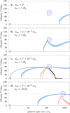 |
Fig. 3 Locations and widths of secular spin–orbit resonances for the exoplanet HIP 41378 f for different parameters of a hypothetical moon. The moon is placed on its Laplace equilibrium plane at a fixed distance from the planet (see labels). The three resonances reachable appear in blue, red, and green. They correspond to the resonances labeled s3, s6, and s1 by Saillenfest et al. (2023). The hatched blue zone is the E1 region where the classic Laplace plane of the moon is unstable. The magenta circle highlights the fully relaxed state of the planet (ω = np and θ ≈ 0). Panel c additionnaly shows the black trajectory from Fig. 2: the system evolves from right to left; the moon is lost in the E1 region, then the planet fully relaxes due to tidal dissipation. |
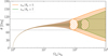 |
Fig. 4 Plot of the E1 region for two different values of am/Rp. For a planet born rapidly rotating, no moon will be found in the shaded regions of parameter space, as otherwise passage through the E1 region during the planet’s tidal despinning and alignment occurs. The E1 region can also be encountered due to lunar migration if the lunar migration timescale is faster than the planet’s despinning timescale. In this case, the moon is lost if the planet’s obliquity lies within about 69◦ and 111◦ (i.e. between the black dashed lines) independent of am/Rp. |
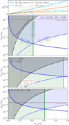 |
Fig. 5 Different mechanisms of moon loss as a function of the system’s parameters. The top panel shows the instability limit (am = 0.36 rH) for a Super Earth-like and Jupiter-like planet in solid lines, and the midpoint radius rM (evaluated with the planet spinning at 2/3 its maximal rate) in dashed lines. The second panel shows the regions of parameter space for the lunar mass ratio (mm/mp) and planet semi-major axis (ap) for a typical super Earth (SE). The gray region above the black dashed line is where moons are lost anyway through runaway migration (Barnes & O’Brien 2002). The vertical green line denotes the boundary between where planets do and do not despin within ∼1 Gyr (Eq. (10)). The blue solid curve denotes the boundary where lunar tidal migration (Eq. (29)) and tidal planet despinning result in comparable changes to am/rM (Eq. (34)): above this curve, E1 is crossed due to lunar migration; below this curve, E1 is crossed due to planetary despinning. The blue dashed line denotes the boundary where lunar tidal migration results in significant changes to am/rM in ∼ Gyr timescales. Accordingly, the region where moons are lost due to lunar migration (with or without capture in secular spin–orbit resonance) is shaded blue, and the region where moons are lost due to planetary despinning is shaded green. The vertical purple line denotes the point at which rM = 5Rp (Eq. (33)). The middle panel is the same for the parameters of Kepler-79d, and the red cross denotes the fiducial parameters adopted for a hypothetical moon (see Fig. 6). The bottom panel is the same for a Jupiter-mass planet. |
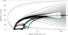 |
Fig. 6 Self-consistent obliquity and spin rate evolution for several realizations of exoplanet Kepler-79 d. Trajectories go from right to left. The planet is initalized with a spin rate of 7.5 hours (i.e. ω/np ≈ 170) and different obliquities equispaced in cos θ. A moon with mass mm/mp = 10−6 is initialized at a distance am = 4 Rp. Integrations are stopped when the moon’s pericenter goes below the Roche limit. The three largest resonances reachable by Kepler-79 d appear in red, blue, and green. The hatched blue zone is the E1 region. For definitiveness, the resonances and E1 region in the background are drawn assuming that the moon is on a circular orbit at am = 4 Rp; for moons that do not cross the E1 region, this remains approximatively true during the whole simulation. |
5 Moons and spin-axis dynamics of despun planets
In this section, we examine the effect of lunar migration on the spin evolution of tidally despun planets, that is, when the planet is close to spin–orbit synchronization. This corresponds to the late-time regime of the same τp ≪ τm limit considered in Section 4. While lunar migration can have dramatic effects on the obliquities of distant fast-spinning planets (e.g., Saillenfest et al. 2021a, 2023), its impact on close-in despun planets remains to be investigated.
5.1 Obliquity equilibria broken by moon inspiral
Around slowly spinning planets, moons all migrate inwards due to tidal dissipation – irrespective of whether the moon is pro-grade or retrograde. When the moon is sufficiently close to the planet, the tide it raises on the planet dominates the tide raised by the star. By comparison of Eqs. (10) and (30), we find that this occurs when the lunar semi-major axis is smaller than the critical value am,crit satisfying:
 (35)
(35)
 (36)
(36)
When the moon is at a distance am,crit from the planet, its orbital angular momentum Lm can quite easily be comparable to the spin angular momentum Sp of the despun planet:
 (37)
(37)
As such, as the moon inspirals, the spin of the planet tends to synchronize with the orbit of its moon. The runaway lunar inspiral stops either when the moon is tidally disrupted below the Roche limit, or when the planet becomes tidally synchronized to the moon. For typical lunar mass ratios (mm ≲ 10−3mp), the latter is impossible, as the moon’s orbit does not contain enough angular momentum to spin up the planet before being disrupted (the classic Darwin instability; Darwin 1879; Makarov & Efroimsky 2023). Nevertheless, the migration of moons can still appreciably change the final spin states of planets.
As discussed in Section 2, a moon-less planet in a multi-planetary system tidally evolves toward one of two tidal Cassini Equilibria (Levrard et al. 2007; Su & Lai 2021), one at low obliquity (tCE1) and one at high obliquity (tCE2). After the planet has reached one of these tCE due to the stellar tide, we now consider the effect of the runaway lunar inspiral. If a prograde moon undergoes runaway inspiral around a planet in tCE1 (θ ≈ 0◦ and ω/np ≈ 1), then the moon simply spins the planet up for a short amount of time without changing its obliquity. Then, after the moon has been disrupted below the Roche limit, the planet converges back to ω/np = 1.
On the other hand, if runaway lunar inspiral occurs around a planet in tCE2 (high obliquity, subsynchronous spin), both the spin rate and obliquity of the planet can be affected. We expect that the moon’s tidal torque, which grows as it inspirals, rapidly overwhelms the spin–orbit resonance (see Sect. 2.3), with the result of ejecting the planet out of tCE2. In such cases, the planet’s spin then aligns with the lunar orbit. Eventually, after the moon is disrupted below the Roche limit, the planet tidally evolves to another equilibrium state.
In order to investigate this scenario, we ran additional simulations with the model of Sect. 2.7, still taking into account the tidal dissipation due to both the star and the moon self-consistently following the constant time-lag theory. We adopt the following parameters: the star has mass m⋆ = 1 M⊙, the planet has mass mp = 10 M⊕, semi-major axis ap = 0.4 au, and zero eccentricity. The moon has mass mm/mp = 3 × 10⁻⁴; it is initialized on its Laplace plane (see below) with 10−4 seed eccentricity. The planet’s Love number is set to k2 = 0.29 and constant time-lag ∆t = 7 × 10⁻⁵ years. The system is perturbed by a 1 MJ planet at 10 au inclined by 10◦, which generates a large secular spin–orbit resonance. In order to produce a (probabilistic) capture into resonance, the planet is initialized with a retrograde obliquity θ ≈ 150◦ and spin period 2π/ω ≈ 5 hours. We note that, for initially retrograde-spinning planets, the lunar orbit in the P1 Laplace state is retrograde with respect to the spin of the planet (im1 > 90◦, point S1 in Fig. 1). Thus, for completeness, we consider both initially prograde (P−1) and retrograde-orbiting (P1) moons as initial conditions.
First, we consider the case in which the orbit of the moon is initially prograde with respect to the planet’s spin; this would be expected if the moon forms from the same disk of material as does the planet, and corresponds to the Laplace equilibrium P−1. The resulting evolution is shown in Fig. 7. The moon first migrates outward, because it is initially located beyond the synchronous radius. However, as the spin rate of the planet is still high, the amount of angular momentum extracted by the moon is negligible. The tidal evolution of the planet is driven by the stellar tides, which damp the planet’s obliquity and spin rate. In this example, the planet is captured in the secular spin–orbit resonance, and it converges toward the tidal Cassini Equilibrium tCE2, in a similar way to moon-less planets (Levrard et al. 2007; Su & Lai 2021). During this process, the moon’s migration is stalled at am ≈ 25 Rp. As the planet’s obliquity and oblateness vary, the moon’s orbital plane adiabatically follows the orientation of the Laplace plane P−1 (see Eq. (20)). For about 100 Myr, the system remains at tCE2 with no much variation, except that the moon slowly inspirals toward the planet. When the moon reaches a distance of am ≈ 15 Rp, however, it starts its runaway inspiral and its angular momentum exchange with the planet becomes more efficient. This ejects the planet out of tCE2. Because at tCE2 the moon is now retrograde to the planet’s spin axis (see left panel of Fig. 1), the moon’s runaway inspiral initially spins the planet further down, and it drives the planet’s spin axis toward θ ≈ 180◦, that is, toward alignment with the (retrograde) moon’s orbital angular momentum. Yet, once the planet’s obliquity goes back to values θ > 90◦, the moon’s orbit is prograde again to the planet’s spin axis, and the moon’s inspiral spins the planet back up. At the end of the moon’s runaway inspiral, the planet’s spin angular momentum and the moon’s orbital angular momentum are approximatively aligned, and the planet’s obliquity is θ ≈ 180◦. At that point, the moon reaches the planet’s Roche limit (considered here to be 2 Rp): we assume that the moon is instantly disrupted into pieces that collide with each other and efficiently damp the remaining angular momentum of the moon. The spin dynamics of the – now moon-less – planet is then driven by stellar tides only. In the example of Fig. 7, the planet is trapped again in Cassini State 2, and it eventually converges back to tCE2.
The peculiar evolution of the system observed here reveals the decisive role of the moon’s angular momentum during its runaway inspiral, despite the modest mass of the moon mm/mp = 3 × 10⁻⁴. As a variant scenario, we wonder what would be the effect of a prograde inspiralling moon, which would spin the planet up at tCE2 (instead of spinning it down), and align its spin axis toward θ ≈ 0◦ (instead of 180◦). The result is shown in Fig. 8. In order for the moon’s orbit to be prograde to the planet’s spin axis at tCE2, we initialize it at the Laplace equilibrium P1. Such a ‘regular retrograde’ moon can be formed as a result of a giant impact that would have tilted the planet to such a large initial obliquity (see e.g. Morbidelli et al. 2012). Contrary to the previous case, the moon initially migrates inwards – because it is retrograde; then, it still migrates inwards when the planet has reached tCE2 – because it is prograde and located below the synchronization radius. Again, the system remains at tCE2 for about 100 Myr, while the moon slowly inspirals. However, when the moon starts its runaway inspiral, it gives angular momentum to the planet and strongly torques its spin axis toward θ ≈ 0◦, which breaks the resonance. When the moon reaches the Roche limit, the planet’s spin angular momentum and the moon’s orbital angular momentum are approximatively aligned, with the planet’s obliquity now θ ≈ 0◦. The stellar tide then directly drives the planet to the tCE1 state, with θ ≈ 0◦ and ω/np ≈ 1. Hence, in this example, the moon’s inspiral and disruption has changed the equilibrium spin state of the planet from a high obliquity to a low obliquity.
The reversed situation can be obtained if the planet initially has a low obliquity – in that case, the existence of a retrograde moon can be explained by a captured object like Triton around Neptune. Figure 9 shows that the planet first converges to tCE1, but it is then ejected by the moon’s runaway inspiral, and it eventually stabilizes at tCE2.
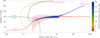 |
Fig. 7 Example of ejection from a tidal Cassini Equilibrium due to moon inspiral. The color of the curve shows the moon’s distance to the planet; the gray curve shows the evolution after the moon has been lost. The center of the resonance (Cassini state 2; red curve) and its width (pink region) are shown at capture time, when the moon’s semi-major axis is am ≈ 25 Rp. Along the dashed black curve, the star-driven tidal dissipation results in |

5.2 Long-lived high obliquity due to moon-driven spin up
Above, we pointed out that moons with typical mass ratios mm/mp ≲ 10−3 experience runaway inspiral and are disrupted before they can tidally synchronize their host planets. However, when the lunar mass is sufficiently large, the moon can considerably spin up and realign the planet (Makarov & Efroimsky 2023; Makarov & Efroimsky 2025), introducing new possibilities for spin–orbit resonances. We consider this possibility here.
As the moon synchronizes the planet, conservation of angular momentum of the moon-planet system demands that the new spin rate of the planet ωnew (also equal to the new mean motion of the moon) satisfies
![Mathematical equation: ${m_{\rm{m}}}\sqrt {G{m_{\rm{p}}}{a_{{\rm{m}},{\rm{crit }}}}} \approx \left[ {{k_{\rm{p}}}{m_{\rm{p}}}R_{\rm{p}}^2 + {m_{\rm{m}}}{{\left( {G{m_{\rm{p}}}/\omega _{{\rm{new }}}^2} \right)}^{2/3}}} \right]{\omega _{{\rm{new }}}},$](/articles/aa/full_html/2026/01/aa55433-25/aa55433-25-eq49.png) (38)
(38)
![Mathematical equation: $\sqrt {{{{a_{{\rm{m}},{\rm{crit }}}}} \over {{R_{\rm{p}}}}}} \approx \left[ {{k_{\rm{p}}}{{{m_{\rm{p}}}} \over {{m_{\rm{m}}}}} + {1 \over {\tilde \omega _{{\rm{new }}}^{4/3}}}} \right]{{\tilde \omega }_{{\rm{new }}}}.$](/articles/aa/full_html/2026/01/aa55433-25/aa55433-25-eq50.png) (39)
(39)
Here,  (Eq. (36)), and we have neglected the contribution of the planet’s spin angular momentum to the initial angular momentum budget (see Eq. (37)). A solution for
  only exists if the minimum of the right-hand side is less than the left-hand side, which requires (cf. Makarov & Efroimsky 2023)
 (40)
(40)
Note that this is a significantly more massive moon than used previously in our fiducial parameters. For an insufficiently massive moon, the right-hand side of Eq. (39) always exceeds the left-hand side, and the moon is tidally disrupted by the planet before it synchronizes the planet’s spin. In contrast, for a sufficiently massive moon, the new planetary spin rate is given by the smaller root of Eq. (39), which yields
 (41)
(41)
 (42)
(42)
This estimate neglects the solar tide during the moon-driven spinup; when including the spindown driven by the solar tide, ωnew will be somewhat lower than this. Note that this result seems somewhat counter-intuitive at first glance: a more massive moon spins the planet up less! There is a simple explanation: for a more massive moon, spinning up the planet requires a smaller change to the lunar orbit, resulting in a smaller lunar mean motion (and planetary spin rate).
Once the massive moon has synchronized the planet, the planet-moon system is in an equilibrium of the lunar tidal evolution. As such, further evolution of the planet’s spin proceeds due to the stellar tide, which acts to weakly drive the planet back to its orbital frequency. Since the lunar tidal torque is stronger than the stellar one, the planet’s spin angular momentum lost to the stellar tidal torque is rapidly replenished by the moon’s orbital angular momentum. Due to the large mass and angular momentum of the moon, this significantly extends the lifetime of the planet’s supersynchronous spin state. However, once even the moon’s angular momentum is depleted by the stellar tide, the moon is tidally disrupted, and the planet rapidly evolves to a tCE following the moon-less spin–orbit evolution (see Sects. 2.1 and 2.2).
This peculiar effect of massive moons prompts us to investigate whether such moons are able to not only produce long-lived supersynchronous spin states, but also high obliquities. As discussed in Sect. 2, lunar migration can change the planet’s spin–orbit coupling frequency, and introduce new possibilities for resonant interactions. In Fig. 10, we illustrate an example of a planet’s spin evolution under the influence of a massive moon with mm/mp = 8 × 10⁻³. We adopt the same parameters as for Figs. 7–9 except that the perturbing planet is located closer in (at 3 au), which moves the spin–orbit resonance to the right of the figure. It can be seen that the initial location of tCE2 is at a relatively low obliquity (red curve). However, as the moon gradually inspirals, two effects occur: (i) am decreases, and (ii) rM increases as the planet is spun up. Both of these effects shift the spin–orbit resonance toward lower values of ω (blue curve). Therefore, as the planet adiabatically follows the location of Cassini state 2, its obliquity increases due both to the moon’s migration and to the planet’s spin up. When the moon-induced tidal dissipation becomes too strong, however, the resonance is broken. The planet then rapidly spins up, and its obliquity damps to zero by the time the moon is disrupted below the Roche limit.
Even though the obliquity increase discussed here is only temporary, it can still persist for millions of years. Figure 11 shows the evolution of the planet’s obliquity and spin rate over time. We see that ω reaches a long-lived steady state: the pseudo-synchronization with the moon (see Eq. (13)), for which ω/nm ≈ 2 cos im/(1 + cos2 im), where im is the inclination of the moon’s orbit with respect to the planet’s equator (where im ≈ im1 is large, see Eq. (18)).
The reason for the somewhat short lifetime of the oblique state can be seen in the bottom panel of Fig. 11: am continues decreasing, rather than reaching a tidally-locked equilibrium. This is because im generally remains large even after the planet spins up, since the moon remains outside the planet’s Laplace radius:
 (43)
(43)
As such, the moon remains on a significantly inclined orbit, far from the tidal equilibrium of the planet-moon system, and the ongoing lunar tide in the planet results in lunar inspiral after several millions of years.
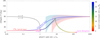 |
Fig. 10 Example of evolution toward a temporary high obliquity due to inspiral of a moon with mass ratio mm/mp = 8 × 10⁻³. Symbols have the same meaning as in previous figures. The system is initialized at tCE2 and the evolution after the moon’s disruption is not shown. In red, we show the resonance at initial time (for am = 25 Rp); in blue, we show the resonance when CS2 is broken (am ≈ 17 Rp). |
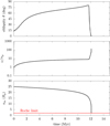 |
Fig. 11 Time evolution of the three quantities shown in Fig. 10: the planet’s obliquity θ, the planet’s spin rate ω, and the moon’s semi-major axis am. |
6 Conclusion
6.1 Summary and discussion
Moons affect the spin-axis dynamics of their host planets. Even the moons of the Solar System giant planets, which only have moon-to-planet mass ratios of the order of 10−4 or less, contribute very significantly to the spin-axis precession rate of their planets. As the orbits of moons expand or contract due to tidal dissipation, moons can have a decisive effect on the planet’s spin-axis dynamics, and in particular increase the planet’s obliquity. This intricate dynamical system can lead to complex outcomes, as the ejection or disruption of the moon. So far, this process has been studied for long-period planets, which are not affected by star–planet tidal dissipation (see e.g., Saillenfest et al. 2021a, 2023).
The spin-axis dynamics of short-period planets is largely influenced by star–planet tidal dissipation, which tends to synchronize the planet’s spin rate to its orbital frequency and damp its obliquity. Yet, high-obliquity states do exist. Tidal dissipation creates new kinds of equilibria (Su & Lai 2021; Yuan et al. 2025); it can either have a destabilising or stabilising influence (Su & Lai 2022). So far, the spin dynamics of short-period planets has been limited to planets without moons, even though moons can readily been formed around short-period planets.
Here, we have investigated the coupled dynamics of warm planets (with periods of about 10 to 200 days) and their moons. We have focused both on the spin dynamics of the planet and the fate of its moon. Depending on the hierarchy of timescales between the star–planet tidal dissipation τp (which synchronizes the planet’s spin rate and damps its obliquity) and the moon-planet tidal dissipation τm (which produces the orbital migration of the moon), a variety of possible evolutions can occur.
First, for moderately short-period planets, for which τp ≳ τm, the star–planet tidal dissipation is noticeable but it unfolds on a longer timescale than the moon’s migration. In that case, our results show that the planet-moon coupled dynamics described in previous works (see e.g., Saillenfest & Lari 2021; Dbouk & Wisdom 2023) still applies, but it is accelerated: see Sect. 3 and Fig. 2. In other words, the migration of the moon is still able to trigger a secular spin–orbit resonance and increase the planet’s obliquity, but the migration range needed for the moon is reduced. Consequently, as compared to long-period planets for which τp ≫ τm, a larger proportion of moderately short-period planets should have been tilted and possibly have lost their moons through the final unstable phase (see Saillenfest et al. 2022, 2023). The resulting planets have large obliquities θ ≳ 80◦ that persist during the lifetime of their planetary systems, because τp is not short enough to damp the obliquity over billions of years. These findings enlarge the parameter space where moon-driven obliquity excitations are possible, together with the potential formation of very inclined rings (see Saillenfest et al. 2023).
Second, we show that lunar orbital destabilization occurs more readily than predicted by previous works (e.g., Barnes & O’Brien 2002; Tremaine et al. 2009; Saillenfest & Lari 2021). In particular, the dynamically unstable E1 region (which occurs for moons with am ≃ rM orbiting planets with obliquities ≃90◦, Tremaine et al. 2009) can be reached with the star–planet tidal dissipation alone, even if the moon’s migration is negligible. This is due to a combination of several factors: First, the Laplace radius, which sets the moon’s dynamical regimes, scales as ω2/5, where ω is the planet’s spin rate, so a decrease in ω is equivalent to an effective outward moon migration. Second, in the process of damping a planet’s obliquity, the star–planet tidal dissipation initially makes the obliquity converge toward 90◦ (see Eq. (9)), where the E1 region lies. This property implies that short-period planets, for which τp ≪ τm, have a natural tendency to loose their moons by forcing them to cross the E1 region. This significantly increases the parameter space where moons are lost compared to existing results (Barnes & O’Brien 2002): Fig. 5 summarizes the analytical boundaries between the different regions of the parameter space where each of moon loss dominates.
Third, for moons that survive the planet’s star-driven tidal despinning stage of evolution, interesting dynamical effects can then occur. As τp ≪ τm for short-period planets, the stellar tides first make the planet converge to one of the two tidal Cassini equilibria, tCE1 or tCE2, as they would do for a moon-less planet in a multiplanetary system (see Su & Lai 2021). The resulting planet has a slow rotation, close to spin–orbit synchronization, and is in a stable state, either with a low obliquity (tCE1) or high obliquity (tCE2). Yet, the moon slowly migrates inwards due to the planet-moon tidal dissipation with timescale τm. This stage can last several hundreds of million years, depending on the parameters of the moon, until the moon enters in a phase of runaway inward migration. At this point, the moon’s orbital angular momentum dominates the planet’s spin angular momentum (even for small moons with masses mm ≲ 10−4mp) because the planet spins very slowly. As a consequence, the runaway moon migration ejects the planet from its tidal Cassini equilibrium and temporarily aligns the planet’s spin angular momentum with the moon’s orbital angular momentum. The runaway moon migration ends when the moon is disrupted below the Roche limit, after which the star–planet tidal dissipation makes the planet converge again toward tCE1 or tCE2. This kind of evolution shows that exomoons, even when they no longer exist today, strongly affect the dynamical history of exoplanets. The migration of moons can eject planets out of spin–orbit equilibria and make them converge to a different equilibrium. We conclude that the demographics of exomoons represent a crucial uncertainty in theoretical predictions of the present-day obliquities of warm exoplanets.
In addition to small moons, with mass ratios comparable to those of moons around the Solar system giant planets (mm ≈ 10−4mp), we have also considered the case of big moons, with mass ratios comparable to that of the Earth’s Moon (mm ≈ 10−2mp). For such big moons, the moon-planet tidal dissipation is strong enough to spin the planet all the way up to synchronization with the moon’s orbit. This process is yet another pathway to a high planetary obliquity through a capture in secular spin–orbit resonance. Contrary to previous scenarios (see e.g., Saillenfest et al. 2021a) the obliquity increase here is primarily due to variations in the planet’s spin rate and oblateness, and not to the moon’s actual migration. Such high obliquity states are transient, because the moon still slowly migrates inwards toward the Roche limit, but they can be relatively long-lived, of the order of tens of millions of years.
6.2 Caveats and future work
Throughout this paper, we have assumed that the lunar orbital evolution is driven by the standard constant time lag prescription, and the stellar and lunar tides are modeled self-consistently according to the same prescription. More complex rheologies and tidal models may result in different evolutionary behaviors compared to those shown in Sections 4 and 5 (in particular in Figs. 6–11). Most importantly, the tidal frequencies of the lunar and planetary orbits differ significantly, suggesting that they may have significantly different dissipation rates when more physically motivated (frequency-dependent) tidal models are adopted. The impact of adopting such an approach is not immediately clear, and future work will be required to understand whether qualitatively new behaviors are found. However, we note that some of the other key dynamical evolutionary features necessary for our work are qualitatively present under more complex rheologies, specifically (i) obliquity excitation at rapid spins and obliquity damping at near-synchronous ones (Boué et al. 2016; Valente & Correia 2022) as well as (ii) the presence of high-obliquity tidally-stable equilibria (Boué 2020).
Additionally, a resonance lock between the lunar orbit and planet’s oscillation modes may result in accelerated orbital evolution of the moon, an effect tentatively supported by Solar System observations (Fuller et al. 2016; Lainey et al. 2020). Such a mechanism is particularly feasible in our scenario if the moon experiences a resonance lock with an inertial mode of the planet: since inertial mode frequencies scale with the planet’s rotation frequency, the planet’s spindown would cause the inertial mode frequencies to decrease, raising the lunar semi-major axis (Fuller et al. 2016). While the role of resonance locks in stellar and/or lunar tides is still not fully well-characterized, more realistic tidal models including resonance locks may change the hierarchy of timescales between τp and τm. The limits of the different regimes derived in this paper and shown in Fig. 5 should therefore not be interpreted as very precise boundaries, but as indicative guidelines for the different regimes of tidal evolution.
Finally, as a third caveat of our tidal model, we neglect cross tides, which arise due to the torque exerted by the tidal bulge raised on the primary by one perturber on a second perturber, as first pointed out in Goldreich (1966) but often omitted without mention in subsequent works on lunar dynamics. The detailed analysis for why this effect can be neglected are somewhat complex (see Appendix A), but the broad reason for its omission is that cross tides are subdominant to the solar-tide-driven planetary spindown as long as the planetary spindown is not significantly slower than the lunar-tide-driven lunar migration.
We have focused here on fluid planets. For rocky planets, their nonzero rigidity would allow them to support J2 moments in excess of their hydrostatic values. For Earth and Venus-like planets, this contribution places a lower bound on their J2 values of ∼4 × 10⁻⁶ (Yoder 1995). For an Earth-like planet at 0.4 au as we used here in our fiducial parameters, this would result in a minimum Laplace radius of
 (44)
(44)
Around such planets, our assertion that the Laplace radius lies within the planet for tidally despun planets is no longer accurate. In such cases, the second crossing of the Laplace radius as the moon tidally inspirals may give rise to additional cases of interesting evolution. However, the maximum asphericity that can be supported by rigidity scales with the dimensionless effective rigidity (Murray & Dermott 1999; Zanazzi & Lai 2017; Yuan et al. 2025)
 (45)
(45)
where µ is the shear modulus of the planet,  is its surface gravity, and ρp its density. Thus, for planets more massive than a few M⊕, the maximum
  decreases sufficiently that rM,min ≲ Rp, and the conclusions in the our study remain qualitatively accurate.
Throughout this work, we have assumed that the putative close-in exoplanets form in their current locations with moon systems resembling those of Solar System planets. However, orbital migration and even instability are thought to occur in many exoplanetary systems, ideas dating back to the proposed disk-driven migration of hot Jupiters (Lin et al. 1996) and still relevant in the context of the formation and breaking of planetary resonant chains (Izidoro et al. 2017; Li et al. 2025). The survival of exomoons through such an active phase of planet formation remains an open question. In this vein, a recent work (Bolmont et al. 2025) considered the survival of exomoons around close-in giant planets during disk-driven migration (paralleling earlier work by Trani et al. 2020 for exomoon survival during high-eccentricity migration formation of hot Jupiters). Our results are complementary to this existing body of literature, focusing on the long-term survival (∼Gyr) of exomoons after other obstacles to their existence during the early phases of the planet’s lifetime.
In this paper, we have not considered tidal dissipation in the moon’s interior and the associated circularization of the moon’s orbit. This would have required to track the moon’s own spin-axis dynamics. With such a more detailed model, our results would remain qualitatively unaffected because the dynamical evolution timescale of the moon (including the destabilization in the E1 region) is very fast, of the order of 100 yr, as compared to the millions of years needed for tidal eccentricity damping (see Sect. 2.7). Yet, including dissipation in the moon’s interior would be needed to determine the actual ultimate fate of the moon when it becomes unstable, whether it is ejected from the planet or disrupted within the Roche limit. In this last case, dedicated simulations (see e.g. Hyodo et al. 2017) can be used to assess how the angular momentum of the moon is removed, either through collisions among the debris, or by transfer to the planet.
Finally, we have only considered here the dynamical effects of a single moon. Multiple major moons, as those of Jupiter, would potentially produce more complex dynamical evolutions, with inner moons migrating faster and dynamically interacting with outer moons. If a given moon is destabilized by passing through the E1 region, it could also produce a chain reaction among other moons and generate a complicated reorganization of the moon system. These possibilities open the door to many more interesting evolution pathways, and draw us back to the conclusion that the possible existence of exomoons, for which we have no statistics yet, is a confounding factor in obliquity predictions.
Acknowledgements
We thank the referee for detailed and insightful comments that improved the quality of this manuscript. YS thanks Daniel Fabrycky, Gongjie Li, and Scott Tremaine for useful discussions. YS acknowledges support by the Lyman Spitzer Jr. Postdoctoral Fellowship at Princeton University and by the Natural Sciences and Engineering Research Council of Canada (NSERC) [funding reference CITA 490888-16]. The authors acknowledge funding by Paris Observatory Research Council for a research stay of YS at Paris Observatory.
References
- Alexander, M. 1973, Astrophys. Space Sci., 23, 459 [Google Scholar]
- Barnes, J. W., & O’Brien, D. 2002, ApJ, 575, 1087 [NASA ADS] [CrossRef] [Google Scholar]
- Batygin, K. 2018, AJ, 155, 178 [NASA ADS] [CrossRef] [Google Scholar]
- Bolmont, E., Galantay, E., Blanco-Cuaresma, S., Oza, A. V., & Mordasini, C. 2025, A&A, 704, A9 [NASA ADS] [CrossRef] [EDP Sciences] [Google Scholar]
- Boué, G. 2020, Celest. Mech. Dyn. Astron., 132, 21 [CrossRef] [Google Scholar]
- Boué, G., & Laskar, J. 2006, Icarus, 185, 312 [Google Scholar]
- Boué, G., & Laskar, J. 2010, ApJ, 712, L44 [CrossRef] [Google Scholar]
- Boué, G., Correia, A. C. M., & Laskar, J. 2016, Celest. Mech. Dyn. Astron., 126, 31 [CrossRef] [Google Scholar]
- Bryan, M. L., Chiang, E., Bowler, B. P., et al. 2020, AJ, 159, 181 [Google Scholar]
- Bryan, M. L., Chiang, E., Morley, C. V., Mace, G. N., & Bowler, B. P. 2021, AJ, 162, 217 [NASA ADS] [CrossRef] [Google Scholar]
- Colombo, G. 1966, AJ, 71, 891 [Google Scholar]
- Correia, A. C. M., & Laskar, J. 2001, Nature, 411, 767 [Google Scholar]
- Correia, A. C. M., Laskar, J., Farago, F., & Boué, G. 2011, Celest. Mech. Dyn. Astron., 111, 105 [NASA ADS] [CrossRef] [Google Scholar]
- Darwin, G. H. 1879, Proc. Roy. Soc. Lond. Ser. I, 29, 168 [Google Scholar]
- Dbouk, R., & Wisdom, J. 2023, PSJ, 4, 188 [Google Scholar]
- Dones, L., & Tremaine, S. 1993, Icarus, 103, 67 [NASA ADS] [CrossRef] [Google Scholar]
- Efroimsky, M., & Lainey, V. 2007, J. Geophys. Res. (Planets), 112, E12003 [NASA ADS] [CrossRef] [Google Scholar]
- Eggleton, P. 2006, Evolutionary Processes in Binary and Multiple Stars, 40 (Cambridge University Press) [Google Scholar]
- Fabrycky, D. C., Johnson, E. T., & Goodman, J. 2007, ApJ, 665, 754 [Google Scholar]
- Farhat, M., Auclair-Desrotour, P., Boué, G., & Laskar, J. 2022, A&A, 665, L1 [NASA ADS] [CrossRef] [EDP Sciences] [Google Scholar]
- Ferraz-Mello, S. 2013, Celest. Mech. Dyn. Astron., 116, 109 [Google Scholar]
- Ferreira, D., Marshall, J., O’Gorman, P., & Seager, S. 2014, Icarus, 243, 236 [Google Scholar]
- Ferraz-Mello, S., Beaugé, C., Folonier, H. A., & Gomes, G. O. 2020, Eur. Phys. J. Spec. Top., 229, 1441 [Google Scholar]
- French, R. G., Nicholson, P. D., Cooke, M. L., et al. 1993, Icarus, 103, 163 [Google Scholar]
- Fuller, J., Luan, J., & Quataert, E. 2016, MNRAS, 458, 3867 [Google Scholar]
- Greene, T. P., Bell, T. J., Ducrot, E., et al. 2023, Nature, 618, 39 [NASA ADS] [CrossRef] [Google Scholar]
- Gold, T., & Soter, S. 1969, Icarus, 11, 356 [NASA ADS] [CrossRef] [Google Scholar]
- Goldreich, P. 1966, Rev. Geophys. Space Phys., 4, 411 [Google Scholar]
- Goldreich, P., & Gold, T. 1963, MNRAS, 126, 257 [Google Scholar]
- Goldreich, P., & Peale, S. 1966, AJ, 71, 425 [NASA ADS] [CrossRef] [Google Scholar]
- Goldreich, P., & Soter, S. 1966, Icarus, 5, 375 [Google Scholar]
- Guerrero, N. M., Ballard, S. A., & Su, Y. 2024, ApJ, 975, 256 [Google Scholar]
- Hammond, M., Bell, T. J., Challener, R. C., et al. 2024, AJ, 168, 4 [Google Scholar]
- Hamilton, D. P., & Ward, W. R. 2004, AJ, 128, 2510 [Google Scholar]
- Henrard, J. 1982, Celest. Mech., 27, 3 [Google Scholar]
- Henrard, J. 1993, The Adiabatic Invariant in Classical Mechanics (Berlin, Heidelberg: Springer Berlin Heidelberg), 117 [Google Scholar]
- Henrard, J., & Murigande, C. 1987, Celest. Mech., 40, 345 [Google Scholar]
- Hut, P. 1981, Astron. Astrophys., 99, 126 [Google Scholar]
- Hu, R., Bello-Arufe, A., Zhang, M., et al. 2024, Nature, 630, 609 [NASA ADS] [CrossRef] [Google Scholar]
- Hyodo, R., Charnoz, S., Ohtsuki, K., & Genda, H. 2017, Icarus, 282, 195 [Google Scholar]
- Izidoro, A., Ogihara, M., Raymond, S. N., et al. 2017, MNRAS, 470, 1750 [Google Scholar]
- Jacobson, R. A. 2022, AJ, 164, 199 [NASA ADS] [CrossRef] [Google Scholar]
- Jontof-Hutter, D., Lissauer, J. J., Rowe, J. F., & Fabrycky, D. C. 2014, ApJ, 785, 15 [NASA ADS] [CrossRef] [Google Scholar]
- Kipping, D. M. 2009, MNRAS, 392, 181 [NASA ADS] [CrossRef] [Google Scholar]
- Kipping, D., Bryson, S., Burke, C., et al. 2022, Nat. Astron., 6, 367 [NASA ADS] [CrossRef] [Google Scholar]
- Kisare, A. M., & Fabrycky, D. C. 2024, MNRAS, 527, 4371 [Google Scholar]
- Kite, E. S., Gaidos, E., & Manga, M. 2011, ApJ, 743, 41 [Google Scholar]
- Lai, D. 2012, MNRAS, 423, 486 [NASA ADS] [CrossRef] [Google Scholar]
- Lammers, C., & Winn, J. N. 2024, ApJ, 977, L1 [Google Scholar]
- Laskar, J. 1988, A&A, 198, 341 [NASA ADS] [Google Scholar]
- Laskar, J. 1990, Icarus, 88, 266 [NASA ADS] [CrossRef] [Google Scholar]
- Li, R., Chiang, E., Choksi, N., & Dai, F. 2025, AJ, 169, 323 [Google Scholar]
- Lin, D. N. C., Bodenheimer, P., & Richardson, D. C. 1996, Nature, 380, 606 [Google Scholar]
- Liu, Q., Zhu, W., Zhou, Y., et al. 2025, AJ, 169, 79 [Google Scholar]
- Lobo, A. H., & Bordoni, S. 2020, Icarus, 340, 113592 [Google Scholar]
- Lu, T., Rein, H., Tamayo, D., et al. 2023, ApJ, 948, 41 [NASA ADS] [CrossRef] [Google Scholar]
- Lu, T., Li, G., Cassese, B., & Lin, D. N. C. 2025, ApJ, 980, 39 [Google Scholar]
- Lainey, V., Arlot, J.-E., Karatekin, Ö., & van Hoolst, T. 2009, Nature, 459, 957 [Google Scholar]
- Lainey, V., Casajus, L. G., Fuller, J., et al. 2020, Nat. Astron., 4, 1053 [Google Scholar]
- Laskar, J., & Robutel, P. 1993, Nature, 361, 608 [Google Scholar]
- Laskar, J., Joutel, F., & Robutel, P. 1993, Nature, 361, 615 [Google Scholar]
- Levrard, B., Correia, A. C. M., Chabrier, G., et al. 2007, A&A, 462, L5 [NASA ADS] [CrossRef] [EDP Sciences] [Google Scholar]
- Li, J., Lai, D., Anderson, K. R., & Pu, B. 2021, MNRAS, 501, 1621 [Google Scholar]
- Makarov, V. V., & Efroimsky, M. 2023, A&A, 672, A78 [NASA ADS] [CrossRef] [EDP Sciences] [Google Scholar]
- Makarov, V. V., & Efroimsky, M. 2025, Universe, 11 [Google Scholar]
- Mathis, S., & Le Poncin-Lafitte, C. 2009, A&A, 497, 889 [NASA ADS] [CrossRef] [EDP Sciences] [Google Scholar]
- Millholland, S., & Batygin, K. 2019, ApJ, 876, 119 [Google Scholar]
- Millholland, S., & Laughlin, G. 2018, ApJ, 869, L15 [CrossRef] [Google Scholar]
- Millholland, S., & Laughlin, G. 2019, Nat. Astron., 3, 424 [Google Scholar]
- Millholland, S. C., & Spalding, C. 2020, ApJ, 905, 71 [NASA ADS] [CrossRef] [Google Scholar]
- Morbidelli, A., Tsiganis, K., Batygin, K., Crida, A., & Gomes, R. 2012, Icarus, 219, 737 [NASA ADS] [CrossRef] [Google Scholar]
- Miguel, Y., & Brunini, A. 2010, MNRAS, 406, 1935 [Google Scholar]
- Murray, C. D., & Dermott, S. F. 1999, Solar System Dynamics (Cambridge University Press) [Google Scholar]
- Neron de Surgy, O., & Laskar, J. 1997, A&A, 318, 975 [NASA ADS] [Google Scholar]
- Ohta, Y., Taruya, A., & Suto, Y. 2009, ApJ, 690, 1 [NASA ADS] [CrossRef] [Google Scholar]
- Palma-Bifani, P., Chauvin, G., Bonnefoy, M., et al. 2023, A&A, 670, A90 [NASA ADS] [CrossRef] [EDP Sciences] [Google Scholar]
- Peale, S. J. 1969, AJ, 74, 483 [Google Scholar]
- Penn, J., & Vallis, G. K. 2017, ApJ, 842, 101 [Google Scholar]
- Poon, M., Bryan, M. L., Rein, H., et al. 2024, AJ, 168, 270 [Google Scholar]
- Ragazzo, C., & Ruiz, L. S. 2017, Celest. Mech. Dyn. Astron., 128, 19 [NASA ADS] [CrossRef] [Google Scholar]
- Rogoszinski, Z., & Hamilton, D. P. 2020, ApJ, 888, 60 [Google Scholar]
- Rogoszinski, Z., & Hamilton, D. P. 2021, PSJ, 2, 78 [Google Scholar]
- Saillenfest, M., & Lari, G. 2021, A&A, 654, A83 [NASA ADS] [CrossRef] [EDP Sciences] [Google Scholar]
- Saillenfest, M., Laskar, J., & Boué, G. 2019, A&A, 623, A4 [NASA ADS] [CrossRef] [EDP Sciences] [Google Scholar]
- Saillenfest, M., Lari, G., & Courtot, A. 2020, A&A, 640, A11 [EDP Sciences] [Google Scholar]
- Saillenfest, M., Lari, G., & Boué, G. 2021a, Nat. Astron., 5, 345 [Google Scholar]
- Saillenfest, M., Lari, G., Boué, G., & Courtot, A. 2021b, A&A, 647, A92 [NASA ADS] [CrossRef] [EDP Sciences] [Google Scholar]
- Saillenfest, M., Rogoszinski, Z., Lari, G., et al. 2022, A&A, 668, A108 [NASA ADS] [CrossRef] [EDP Sciences] [Google Scholar]
- Saillenfest, M., Sulis, S., Charpentier, P., & Santerne, A. 2023, A&A, 675, A174 [NASA ADS] [CrossRef] [EDP Sciences] [Google Scholar]
- Safronov, V. S. 1966, Soviet Ast., 9, 987 [NASA ADS] [Google Scholar]
- Sasaki, T., Barnes, J. W., & O’Brien, D. P. 2012, ApJ, 754, 51 [NASA ADS] [CrossRef] [Google Scholar]
- Su, Y., & Lai, D. 2020, ApJ, 903, 7 [Google Scholar]
- Su, Y., & Lai, D. 2021, MNRAS, 509, 3301 [CrossRef] [Google Scholar]
- Su, Y., & Lai, D. 2022, MNRAS, 513, 3302 [NASA ADS] [CrossRef] [Google Scholar]
- Takata, T., & Stevenson, D. J. 1996, Icarus, 123, 404 [NASA ADS] [CrossRef] [Google Scholar]
- Teachey, A., & Kipping, D. M. 2018, Sci. Adv., 4, eaav1784 [Google Scholar]
- Thao, P. C., Mann, A. W., Feinstein, A. D., et al. 2024, AJ, 168, 297 [Google Scholar]
- Tremaine, S. 1991, Icarus, 89, 85 [Google Scholar]
- Tremaine, S., Touma, J., & Namouni, F. 2009, AJ, 137, 3706 [Google Scholar]
- Touma, J., & Wisdom, J. 1993, Science, 259, 1294 [NASA ADS] [CrossRef] [Google Scholar]
- Touma, J., & Wisdom, J. 1994, AJ, 108, 1943 [NASA ADS] [CrossRef] [Google Scholar]
- Touma, J., & Wisdom, J. 1998, AJ, 115, 1653 [NASA ADS] [CrossRef] [Google Scholar]
- Trani, A. A., Hamers, A. S., Geller, A., & Spera, M. 2020, MNRAS, 499, 4195 [NASA ADS] [CrossRef] [Google Scholar]
- Valente, E. F., & Correia, A. C. 2022, A&A, 665, A130 [NASA ADS] [CrossRef] [EDP Sciences] [Google Scholar]
- Vaillant, T., & Correia, A. C. M. 2022, A&A, 657, A103 [NASA ADS] [CrossRef] [EDP Sciences] [Google Scholar]
- Vokrouhlický, D., & Nesvorný, D. 2015, ApJ, 806, 143 [Google Scholar]
- Ward, W. R. 1975, AJ, 80, 64 [Google Scholar]
- Ward, W. R., & Hamilton, D. P. 2004, AJ, 128, 2501 [Google Scholar]
- Ward, W. R., & Canup, R. M. 2006, ApJ, 640, L91 [Google Scholar]
- Wisdom, J., Dbouk, R., Militzer, B., et al. 2022, Science, 377, 1285 [NASA ADS] [CrossRef] [Google Scholar]
- Yahalomi, D. A., Kipping, D., Nesvorný, D., et al. 2024, MNRAS, 527, 620 [Google Scholar]
- Yuan, H. D. A., Su, Y., & Goodman, J. 2025, ApJ, 987, 9 [Google Scholar]
- Yoffe, G., Ofir, A., & Aharonson, O. 2021, ApJ, 908, 114 [NASA ADS] [CrossRef] [Google Scholar]
- Yoder, C. F. 1995, in Global Earth Physics: A Handbook of Physical Constants, ed. T. J. Ahrens, 1 [Google Scholar]
- Zanazzi, J. J., & Lai, D. 2017, MNRAS, 469, 2879 [Google Scholar]
- Zanazzi, J. J., Dewberry, J., & Chiang, E. 2024, ApJ, 967, L29 [Google Scholar]
We note that the sign of σ here is opposite to that of Su & Lai (2021), so our equations of motion are consistent with theirs.
We note that the tidal lag time is sometimes associated with an “effective” tidal quality factor Q via 2np∆t ∼ 1/Q (Lai 2012; Lu et al. 2023).
Strictly speaking, the spin equilibrium has a small nonzero σ, and hence could be called a modified Cassini state to distinguish from the non-dissipative equilibrium (Su & Lai 2021). Since we study only the dissipative dynamics, we refer to them as just Cassini states for the remainder of the work.
Equation (23) also slightly differs from Eq. (39) of Saillenfest & Lari (2021), as we have removed an absolute value. This absolute value was put by Saillenfest & Lari (2021) to enforce the moon to always be prograde to the planet’s spin in their calculations, without the need to change the expression of im from im1 to im,−1. We drop this ambiguous notation here and use the classic expression with parentheses (see e.g., French et al. 1993).
More precisely, the linear law assumed here for the moon’s semi-major axis am produces the same variation range ∆am during the integration time as a constant time-lag prescription with ∆t = 3 × 10⁻⁹ yr (see e.g., Efroimsky & Lainey 2007 for the explicit formula).
We note that while we consider only the constant time lag model here (see Sect. 2.2), more general conditions for tidal obliquity excitation can be developed for general equilibrium tidal models (e.g., Boué et al. 2016; Valente & Correia 2022), and obliquity excitation can even arise in dynamical tidal models such as resonance locks (e.g., see appendix of Zanazzi et al. 2024).
Appendix A Cross tides
A rather subtle yet important caveat in our work is the omission of the so-called “cross tidal” interactions (Goldreich 1966; Touma & Wisdom 1994; Neron de Surgy & Laskar 1997; Mathis & Le Poncin-Lafitte 2009). While these interactions are often neglected without explicit consideration, they are known to significantly affect the history of the lunar orbit, as first pointed out by the seminal work of Goldreich (1966). Here, we present an abbreviated discussion of cross tides, focusing on the key results necessary for justifying their omission.
In the standard tidal theory, the [time-lagged] bulge raised by a perturbing body exerts a torque on that same perturber, driving dissipation. However, in systems with at least three bodies, the bulges raised on the primary by one perturber also exert torques on the other perturber[s]. Readers interested in a more complete discussion of this phenomenon are encouraged to refer to Touma & Wisdom (1994), which contains the most complete expressions for the architecture we consider: they do not average over the lunar orbital precession as do Goldreich (1966) and Neron de Surgy & Laskar (1997), which is only appropriate for moons beyond the Laplace radius, such as Earth’s moon today.
The essential effect of cross tides can be understood simply. As above, we consider a three-body system consisting of the star, planet, and moon. In the frame of the planet, the two perturbers are the star, which orbits with frequency np, and the moon, which orbits with frequency nm. We assume that the system is not near any resonances, so np and nm are not commensurate. In each cross tidal contribution, the bulge raised by one body, the “perturbing” body, effects a torque on the other body, the “torqued” body. Then, when averaging over the mean anomalies of both orbits, it is clear that only the axisymmetric components of the gravitational potentials of both the perturbing and torqued bodies can interact in a way that results in a non-vanishing torque. While it is not obvious that time-lagged axisymmetric perturbations can lead to a net torque, this indeed is possible when the two orbits are misaligned (e.g., see Lai 2012 for another example of this).
By recognizing the independence of the cross tidal torques of the bodies’ mean anomalies, we identify one of their key features: they cannot change the magnitudes of the orbital angular momenta in the system (notably, they do not yield lunar migration; see also the explicit torques provided by Touma & Wisdom 1994). Thus, the cross tide results in the planet’s spin axis and torqued body’s orbit normal being driven toward alignment at constant total angular momentum and constant orbital angular momentum magnitude. A complementary decrease of the planet’s spin rate is a consequence of these two constraints. The characteristic evolution timescale of the planet’s spin rate due to cross tides can be written (Goldreich 1966; Touma & Wisdom 1994)
 (A.1)
(A.1)
where τp as given by Eq. (10) is the despinning timescale due to the bulge raised by the star torquing the star. The instantaneous despinning time due to cross tides includes some prefactors, but they generally result in a longer spin evolution timescale than predicted by Eq. (A.1), approaching infinity as the misalignment in the system goes to zero (where there is no cross-tidal torque), toward understanding the effect of cross tides on our results, we turn to a timescale analysis. Note that
 (A.2)
(A.2)
where τp,m is the despinning time due to the lunar bulge torquing the moon (Eq. 30). Since τp,m ∼ τm(Sp/Lm), we see that τp,cross−tide ≲ τp requires τm ≲ τp(Lm/Sp) ≪ τp. In other words, requiring that the cross-tidal despinning timescale be nonnegligible also requires that the lunar migration time be significantly shorter (even more so than the angular momentum ratio Lm/Sp) than the planetary spin evolution timescale. Since the focus of this paper is on regimes where the planetary spin evolution is at least as fast as the lunar migration, we conclude that the cross-tidal evolution is negligible in affecting the planet’s spin evolution in our study. In conjunction with the lack of an effect on the lunar orbit, we justify the omission of cross tides in our study.
Appendix B Evection and eviction resonances
Evection and eviction resonances happen when the apsidal or nodal precession frequencies of a moon are commensurable with the mean motion of its host planet on its orbit around the star (Touma & Wisdom 1998; Vaillant & Correia 2022). These resonances can substantially affect the eccentricity and inclination of a moon; however, these resonances are not included in secular models that are averaged over the orbital motion of the planet. In order to use a secular code (as we do in all the numerical experiments in this paper), we must assert that these resonances cannot be reached, or cannot appreciably change the dynamics at play.
In this paper, we only consider relatively small moons (mm/mp of the order of 10−4) orbiting close to their Laplace equilibrium (see Tremaine et al. 2009). The close proximity to the Laplace equilibrium is indeed verified at all times in our simulations, except when the system enters the E1 region, in which case the moon is rapidly destabilized anyway (see Sect. 4). Therefore, outside of the E1 region, a good approximation to the apsidal and nodal precession frequencies of the moon is given by the frequencies of small oscillations around the Laplace equilibrium. These frequencies have been computed by Tremaine et al. (2009) for a massless moon. We call them µ1 and ξ1, respectively, following Eqs. (19) and (16) of Saillenfest & Lari (2021).
Evection and eviction-like resonances are triggered when the planet’s mean motion np is in an integer commensurability with µ1 or/and ξ1. Vaillant & Correia (2022) give a list of all possible commensurabilities in the quadrupolar approximation. For a given spin rate ω of the planet, we can locate where these commensurabilities occur in the plane (am, θ). By doing so, we note that, for the parameters considered in this paper, evection and eviction-like resonances are all located at distances am significantly closer to the planet than the mid-point radius rM. Consequently, we can simplify the expression of µ1 and ξ1 to
 (B.1)
(B.1)
(see Eqs. B.2 and B.5 of Saillenfest & Lari 2021). By equating µ1 (or −ξ1) with np, we get the nominal location of the evection (or eviction) resonance:
![Mathematical equation: ${{{a_{\rm{m}}}} \over {{R_{\rm{p}}}}} = {\left[ {{{k_2^2} \over 4}{{{m_ \star }} \over {{m_{\rm{p}}}}}{{\left( {{{{R_{\rm{p}}}} \over {{a_{\rm{p}}}}}} \right)}^3}{{\left( {{\omega \over {{n_{\rm{p}}}}}} \right)}^4}} \right]^{1/7}}.$](/articles/aa/full_html/2026/01/aa55433-25/aa55433-25-eq64.png) (B.2)
(B.2)
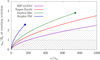 |
Fig. B.1 Distance of the moon at the evection (or eviction) resonance as a function of the spin rate of the planet. The four curves cover all different settings considered throughout this paper. On each curve, the dot shows the planet’s breakup spin rate. The two hatched zones below am/Rp = 1 and am/Rp = 2 show the planet’s radius and approximate Roche limit, respectively. |
As a function of the spin rate of the planet, the resulting distance of the moon is shown in Fig. B.1. We note that, as the planet spins down due to the star-driven tidal dissipation, the location of the evection resonance rapidly drifts below the planet’s own radius. This is because J2 decreases, which slows down the moon’s orbital precession. As a result, the evection or eviction resonances can never be reached by the moon.
Figure B.1 only shows the location of the resonance np + ξ1 = 0. Among the other resonances listed by Vaillant & Correia (2022), some are located farther away from the planet. If we consider the most distant resonance, this adds a factor 32/7 ≈ 1.37 to Eq. (B.2). This distance still remains firmly below the distance of the moon at any point during its evolution. Moreover, for moons close to their Laplace equilibrium, with nearly circular orbits, Vaillant & Correia (2022) note that only the resonances np + ξ1 = 0 and 2np + ξ1 = 0 can have a substantial effect (and the resonance 2np + ξ1 = 0 is located even closer-in than shown in Fig. B.1).
From this discussion, we conclude that evection and eviction-like resonances can safely be ignored throughout this paper. This justifies the use of a secular code averaged over the orbital motion of the planet.
All Figures
|
Fig. 1 Orbital inclinations of Laplace state P1 and its twin P−1 (colorbar, given by Eqs. (18), (20)) as functions of am/rM and the planet’s obliquity θ. In both panels, the location of am = rM is denoted with a vertical black dashed line, and the E1 region (where P1 and P−1 are unstable) is shown by a white hatched zone. Across the two panels, a representative evolutionary history is shown via the three cyan points and arrows (S1, S2, S3). While the inclinations of P1 and P−1 only depend on θ and am/rM, we also illustrate the evolution using the following concrete parameters for interpretability: ap = 0.4 au, ep = 0, Rp = 2 R⊕, and mp = 10 M⊕. We then denote the corresponding values of the planet’s spin rate along the top-left axis (relevant to planetary tidal evolution) and the lunar semi-major axis along the top-right axis (relevant to lunar migration). In the left panel, the planet is initially rapidly rotating with a period of 7.5 hours, and the moon is located at am = 5Rp (S1). Then, as the planet despins and the obliquity damps, rM decreases while the moon is still located at am = 5Rp, and the system reaches S2 (we have neglected lunar tidal migration for illustrative purposes). Going from S1 to S2, the inclination of the lunar orbit smoothly flips from prograde to retrograde (assuming that the moon occupies P−1). In the right panel, as the moon inspirals, starting from S2, am decreases until the moon is disrupted by the planet when am ≃ Rp ≳ rM (S3). |
| In the text | |
|
Fig. 2 Example of obliquity evolution of the planet HIP 41378 f and a hypothetical moon. The mass of the moon is m/M = 7 × 10⁻⁴, and it is initialized at a distance am = 5 Rp. For the red, blue, and black curves, the lunar migration rate is analogous to that measured for Io and Jupiter (Lainey et al. 2009). Dark colors show the trajectory when the moon is still present; light colors show the trajectory after the loss of the moon, assumed to be instantly disrupted once its pericenter goes below the Roche limit. For the red curve, the star–planet tidal dissipation is taken into account with tidal time-lag ∆t = 3×10⁻⁹ years. For the blue curve, the star–planet tidal dissipation is artificially increased using ∆t = 2×10⁻⁴ years. For the black curve, the star–planet tidal dissipation is artificially increased using ∆t = 2 × 10⁻² years. For the green curve, the moon’s migration is turned off, and the star–planet tidal dissipation is taken into account using ∆t = 2 × 10⁻⁴ years. |
| In the text | |
|
Fig. 3 Locations and widths of secular spin–orbit resonances for the exoplanet HIP 41378 f for different parameters of a hypothetical moon. The moon is placed on its Laplace equilibrium plane at a fixed distance from the planet (see labels). The three resonances reachable appear in blue, red, and green. They correspond to the resonances labeled s3, s6, and s1 by Saillenfest et al. (2023). The hatched blue zone is the E1 region where the classic Laplace plane of the moon is unstable. The magenta circle highlights the fully relaxed state of the planet (ω = np and θ ≈ 0). Panel c additionnaly shows the black trajectory from Fig. 2: the system evolves from right to left; the moon is lost in the E1 region, then the planet fully relaxes due to tidal dissipation. |
| In the text | |
|
Fig. 4 Plot of the E1 region for two different values of am/Rp. For a planet born rapidly rotating, no moon will be found in the shaded regions of parameter space, as otherwise passage through the E1 region during the planet’s tidal despinning and alignment occurs. The E1 region can also be encountered due to lunar migration if the lunar migration timescale is faster than the planet’s despinning timescale. In this case, the moon is lost if the planet’s obliquity lies within about 69◦ and 111◦ (i.e. between the black dashed lines) independent of am/Rp. |
| In the text | |
|
Fig. 5 Different mechanisms of moon loss as a function of the system’s parameters. The top panel shows the instability limit (am = 0.36 rH) for a Super Earth-like and Jupiter-like planet in solid lines, and the midpoint radius rM (evaluated with the planet spinning at 2/3 its maximal rate) in dashed lines. The second panel shows the regions of parameter space for the lunar mass ratio (mm/mp) and planet semi-major axis (ap) for a typical super Earth (SE). The gray region above the black dashed line is where moons are lost anyway through runaway migration (Barnes & O’Brien 2002). The vertical green line denotes the boundary between where planets do and do not despin within ∼1 Gyr (Eq. (10)). The blue solid curve denotes the boundary where lunar tidal migration (Eq. (29)) and tidal planet despinning result in comparable changes to am/rM (Eq. (34)): above this curve, E1 is crossed due to lunar migration; below this curve, E1 is crossed due to planetary despinning. The blue dashed line denotes the boundary where lunar tidal migration results in significant changes to am/rM in ∼ Gyr timescales. Accordingly, the region where moons are lost due to lunar migration (with or without capture in secular spin–orbit resonance) is shaded blue, and the region where moons are lost due to planetary despinning is shaded green. The vertical purple line denotes the point at which rM = 5Rp (Eq. (33)). The middle panel is the same for the parameters of Kepler-79d, and the red cross denotes the fiducial parameters adopted for a hypothetical moon (see Fig. 6). The bottom panel is the same for a Jupiter-mass planet. |
| In the text | |
|
Fig. 6 Self-consistent obliquity and spin rate evolution for several realizations of exoplanet Kepler-79 d. Trajectories go from right to left. The planet is initalized with a spin rate of 7.5 hours (i.e. ω/np ≈ 170) and different obliquities equispaced in cos θ. A moon with mass mm/mp = 10−6 is initialized at a distance am = 4 Rp. Integrations are stopped when the moon’s pericenter goes below the Roche limit. The three largest resonances reachable by Kepler-79 d appear in red, blue, and green. The hatched blue zone is the E1 region. For definitiveness, the resonances and E1 region in the background are drawn assuming that the moon is on a circular orbit at am = 4 Rp; for moons that do not cross the E1 region, this remains approximatively true during the whole simulation. |
| In the text | |
|
Fig. 7 Example of ejection from a tidal Cassini Equilibrium due to moon inspiral. The color of the curve shows the moon’s distance to the planet; the gray curve shows the evolution after the moon has been lost. The center of the resonance (Cassini state 2; red curve) and its width (pink region) are shown at capture time, when the moon’s semi-major axis is am ≈ 25 Rp. Along the dashed black curve, the star-driven tidal dissipation results in |
| In the text | |
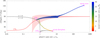 |
Fig. 8 Same as Fig. 7, but with an initially retrograde moon. |
| In the text | |
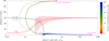 |
Fig. 9 Same as Fig. 8, but for an initially low-obliquity planet. |
| In the text | |
|
Fig. 10 Example of evolution toward a temporary high obliquity due to inspiral of a moon with mass ratio mm/mp = 8 × 10⁻³. Symbols have the same meaning as in previous figures. The system is initialized at tCE2 and the evolution after the moon’s disruption is not shown. In red, we show the resonance at initial time (for am = 25 Rp); in blue, we show the resonance when CS2 is broken (am ≈ 17 Rp). |
| In the text | |
|
Fig. 11 Time evolution of the three quantities shown in Fig. 10: the planet’s obliquity θ, the planet’s spin rate ω, and the moon’s semi-major axis am. |
| In the text | |
|
Fig. B.1 Distance of the moon at the evection (or eviction) resonance as a function of the spin rate of the planet. The four curves cover all different settings considered throughout this paper. On each curve, the dot shows the planet’s breakup spin rate. The two hatched zones below am/Rp = 1 and am/Rp = 2 show the planet’s radius and approximate Roche limit, respectively. |
| In the text | |
Current usage metrics show cumulative count of Article Views (full-text article views including HTML views, PDF and ePub downloads, according to the available data) and Abstracts Views on Vision4Press platform.
Data correspond to usage on the plateform after 2015. The current usage metrics is available 48-96 hours after online publication and is updated daily on week days.
Initial download of the metrics may take a while.