| Issue |
A&A
Volume 705, January 2026
|
|
|---|---|---|
| Article Number | A15 | |
| Number of page(s) | 13 | |
| Section | The Sun and the Heliosphere | |
| DOI | https://doi.org/10.1051/0004-6361/202555912 | |
| Published online | 23 December 2025 | |
The Uniturbulence and Alfvén Wave Solar Model (UAWSoM) in MPI-AMRVAC
1
Centre for mathematical Plasma Astrophysics, Department of Mathematics, KU Leuven, Celestijnenlaan 200B Bus 2400, 3001 Leuven, Belgium
2
Starion Group S.A., Rue des Etoiles 140, 6890 Libin, Belgium
3
Solar-Terrestrial Centre of Excellence – SIDC, Royal Observatory of Belgium, Ringlaan -3- Av. Circulaire, 1180 Brussels, Belgium
★ Corresponding author: This email address is being protected from spambots. You need JavaScript enabled to view it.
Received:
12
June
2025
Accepted:
30
October
2025
Abstract
Context. The coronal heating problem and the generation of the solar wind remain fundamental challenges in solar physics. While approaches based on, e.g., the Alfvén Wave Solar Model (AWSoM) have proven highly successful in reproducing the large-scale structure of the solar corona, they inherently neglect contributions from additional wave modes that arise when the effects of transverse structuring are fully incorporated into the magnetohydrodynamic (MHD) equations.
Aims. In this paper, we compare the respective roles of heating driven by kink waves and Alfvén waves in sustaining a region of the solar atmosphere. We employ newly developed physics and radiative cooling modules within MPI-AMRVAC.
Methods. We extended the existing MHD physics module in MPI-AMRVAC by incorporating additional Alfvén and kink wave energy contributions to the MHD equations. We examined their roles in heating the solar atmosphere and driving the solar wind. To validate our approach, we compared our numerical results from Python-based simulations with those obtained using the UAWSoM module in MPI-AMRVAC. Furthermore, we assessed the heating efficiency of kink waves relative to that of pure Alfvén waves through two parameter studies: (1) exploring how different Alfvén wave reflection rates impact the simulated atmosphere and (2) varying the relative magnitudes of Alfvén and kink wave energy injections. Finally, we present the results of a larger scale domain fully sustained by kink wave-driven heating.
Results. Our results show that kink wave-driven (UAWSoM) models can sustain a stable atmosphere without requiring any artificial background heating terms, unlike traditional Alfvén-only models. We attribute this to the increased heating rate associated with kink waves compared with Alfvén waves, given the same energy injection.
Conclusions. Kink waves have the capacity to sustain a model plasma with temperature and density values representative of coronal conditions, without the need to resort to ad hoc heating terms.
Key words: magnetohydrodynamics (MHD) / turbulence / Sun: corona / Sun: magnetic fields
© The Authors 2025
 Open Access article, published by EDP Sciences, under the terms of the Creative Commons Attribution License (https://creativecommons.org/licenses/by/4.0), which permits unrestricted use, distribution, and reproduction in any medium, provided the original work is properly cited.
This article is published in open access under the Subscribe to Open model. This email address is being protected from spambots. You need JavaScript enabled to view it. to support open access publication.
1. Introduction
The magnetohydrodynamic (MHD) equations offer a theoretical framework through which the dynamic behavior of magnetised plasma can be explored, revealing a rich spectrum of wave solutions as a response to perturbations of various plasma quantities. MHD waves have long been thought to carry energy to higher altitudes of the solar atmosphere (Alfvén 1947), where various dissipative mechanisms are thought to convert magnetic energy into thermal energy, subsequently heating the surrounding plasma.
Perhaps the simplest solution among the wave modes supported by the MHD equations is the pure Alfvén wave (Alfvén 1942). The Alfvén wave solution (as is the case for all wave solutions) is not inherently straightforward due to a single perturbation generally giving rise to both forward and backward (with respect to the magnetic field) propagating wave components. This complicates the analysis of wave dynamics, particularly in nonlinear regimes where counterpropagating waves can interact nonlinearly, leading to the development of turbulence, ultimately leading to the dissipation of wave energy (see, e.g., Matthaeus et al. 1999; Verdini & Velli 2007; Chandran & Hollweg 2009; Chandran et al. 2011). To address this, the Elsässer variables (Elsasser 1950) have proven especially useful, enabling the decomposition of the total perturbation into two distinct fields that can be used to separately track the propagation of wave energy along and against the magnetic field direction, as well as the nonlinear interaction between counterpropagating waves.
The so-called Alfvén Wave Solar Model (AWSoM) proposed by van der Holst et al. (2014) adopted this wave frame variable approach, modeling the evolution and dissipation of Alfvén waves as an additional contribution to the MHD equations. These models are widely employed for space weather forecasting and have been shown to reproduce large-scale properties of the solar wind (e.g., Riley et al. 2019). AWSoM models possess heating terms that contain both Elsässer components, which requires Alfvén wave reflection to generate any non-adiabatic wave heating. Alfvén waves can be excited in the photosphere by convective motions and propagate along the magnetic field lines, whereby stratification can cause partial wave reflection, leading to a source of counterpropagating wave energy. Numerical models often incorporate this by including an analytical reflection term in the Alfvén wave energy evolution equations. This reflection rate is usually defined in terms of the Alfvén speed gradient (van der Holst et al. 2014; Downs et al. 2016) and dictates the proportion of Alfvén wave energy available for contributing to the heating of the plasma. Simple linear models can capture wave reflection due to the presence of longitudinal gradients in the wave speed; however, these models only show significant reflection if the length scale of the inhomogeneity is comparable to the wavelength (Soler 2025). That being said, Morton et al. (2015) presented observational evidence obtained from the Coronal Multi-channel Polarimeter (CoMP) of the existence of counterpropagating Alfvénic waves with around 20–80% of the energy of outward propagating wave energy, depending on the wave frequency (Tomczyk et al. 2007). However, many of these numerical models do not rely solely on Alfvén wave dissipation. They often require anomalous heating functions to produce stable atmospheres. For instance, Mikić et al. (2018) found insufficiently heated regions near magnetic null points and open field lines connected to weak field regions. To circumvent this, they employed two spherically symmetric heating functions to provide extra heating in the low corona. Compressive modes such as acoustic shock waves are thought to play a major role in heating the chromosphere and low corona (Suzuki & Inutsuka 2005, 2006; Cranmer et al. 2007), with Alfvén wave heating playing the role in heating the upper corona. These background heating terms could be thought to replicate the role of these compressive phenomena without introducing other wave modes into the domain to allow for the parameterisation of wave energy in such AWSoM(-like) models. The ability of acoustic waves to heat the chromosphere has received criticism, however, as Beck et al. (2009, 2012) found the wave energy to be insufficient to maintain the temperature of the atmosphere. This naturally leads to one fundamental unanswered question: what physical processes are missing in these models?
Traditionally, turbulent dissipation in magnetised plasmas has long been associated with the nonlinear interaction of counterpropagating pure Alfvén waves. However, the solar atmosphere is highly inhomogeneous and transverse structures have long been observed to extend far into the corona (see, e.g., Raymond et al. 2014; DeForest et al. 2018; Stenborg et al. 2021). This complexity gives rise to a broader spectrum of wave modes supported by the MHD equations (Roberts 1981). Goossens et al. (2019) showed that generally, in inhomogeneous plasmas any perturbation across Alfvén speed isosurfaces has mixed properties. Specifically related to the presence of transverse inhomogeneity, Magyar et al. (2019) demonstrated that surface Alfvén waves possessed both Elsässer components and demonstrated that transverse structuring leads to a nonlinear self-deformation process known as uniturbulence, enabling wave-driven heating without requiring reflected or externally driven counterpropagating waves. Evans et al. (2012) incorporated such surface Alfvén waves into global MHD models and successfully reproduced key observational signatures without invoking an ad hoc heating term, highlighting the critical role of transverse structuring in models of turbulent wave heating. Extending this concept, Van Doorsselaere et al. (2024) developed the Q-variable framework, a generalisation of the Elsässer variables that allows for the decomposition of kink waves into forward- and backward-propagating components, and the authors showed that kink waves have non-zero heating rates in the absence of wave reflection. Much like the Elsässer formulation for Alfvén waves, this approach enables us to analyze turbulent wave dissipation and energy transport in transversally structured plasmas representative of the corona.
The aim of this paper is to advance upon the work conducted by Van Doorsselaere et al. (2025), who numerically investigated the turbulent dissipation of kink waves in a stratified coronal plasma using a newly developed Python code. This implementation serves as a reference implementation for the UAWSoM concept and has been made available on Gitlab1. To build upon this work, we introduced a new physics module called the Uniturbulence and Alfvén wave Solar Model (UAWSoM) into the MPI-AMRVAC framework (Xia et al. 2018; Keppens et al. 2023) to model the nonlinear turbulent dissipation of Alfvén and kink wave energy and the impact this has on a solar atmospheric plasma. We have made a separate repository for UAWSoM in MPI-AMRVAC available on Github2.
The structure of this investigation is as follows. In Section 2, we re-introduce the mathematical formalism introduced by Van Doorsselaere et al. (2024) and set out the equations implemented in this new physics module. In Section 3, we discuss a comparison case between the Python implementation and our new MPI-AMRVAC implementation and present a fully self-consistent equilibrium obtained through kink wave heating without the requirement of an ad hoc heating function. In Sections 4 and 5, we describe the parameter studies we conducted, where we varied the reflection rate of Alfvén waves and the ratio between the Alfvén and kink wave energy injection, respectively. In Section 6, we present simulations extending to 3 R⊙, Section 7 discusses the potential impact of two physical effects: kink wave reflection and resonant absorption. In Section 8, we conclude our results and propose plans for future directions of research.
2. Model description
The macroscopic behavior of a plasma can be described in terms of the MHD equations. In the context of these equations, we consider the additional effects of wave energy on the energy and momentum of the system. To model the evolution of Alfvén and kink wave energy in the solar atmosphere, we used both the Elsässer variables given by Z± = V ± vA and Q variables given by Q± = V ± αB, where V represents the velocity of the fluid, B represents the magnetic field, vA the Alfvén speed, and α a generic placeholder for the speed of other waves, in this case taken to be the kink speed. Introducing these new variables allows for the formulation of the following equations:
 (1)
(1)
 (2)
(2)
 (3)
(3)
![Mathematical equation: $$ \begin{aligned}&\frac{\partial }{\partial t} \left( \rho _0 \frac{V^2}{2} + \frac{p}{\gamma - 1} + \frac{B_0^2}{2\mu } + \sum W_\mathrm{A,k} ^\pm \right) \nonumber \\&+ \nabla \cdot \Bigg ( \left[ \rho _0 \frac{V^2}{2} + \frac{p}{\gamma - 1} + \frac{B_0^2}{2\mu } \right] \boldsymbol{V} - \boldsymbol{B}_0 \frac{\boldsymbol{V} \cdot \boldsymbol{B}_0}{\mu } \Bigg ) \nonumber \\&+ \nabla \cdot \left( \boldsymbol{Z}_0^- W_\mathrm{A} ^+ + \boldsymbol{Z}_0^+ W_\mathrm{A} ^- + \boldsymbol{Q}_0^- W_\mathrm{k} ^+ + \boldsymbol{Q}_0^+ W_\mathrm{k} ^- \right) + \nabla \cdot \left( [P_\mathrm{A} + P_\mathrm{k} ] \boldsymbol{V} \right) \nonumber \\&= - \mathcal{L} - \rho _0 \boldsymbol{V} \cdot \boldsymbol{g}(\boldsymbol{z}) + \frac{\zeta - 1}{\zeta + 1} P_\mathrm{k} \nabla \cdot \boldsymbol{V}, \end{aligned} $$](/articles/aa/full_html/2026/01/aa55912-25/aa55912-25-eq4.gif) (4)
(4)
 (5)
(5)
 (6)
(6)
where μ is the permeability constant, p the hydrodynamic pressure, and PA, k are the additional pressure contributions from Alfvén and kink waves, respectively. These expressions are defined by van der Holst et al. (2014), Van Doorsselaere et al. (2025) as
 (7)
(7)
Continuing the adopted notation, g represents gravity, γ is the polytropic index taken to be 5/3 (corresponding to an ideal monatomic gas with the pressure and density related via p ∝ ργ), WA, k± represents the Alfvén and kink wave energies for inward and outward propagating waves, Z0 and Q0 represent the equilibrium Elsässer and Q-fields, corresponding to the Alfvén and kink speeds, respectively (with B0 the equilibrium magnetic field), ℒ the radiative losses, ζ the density contrast of the plasma between the inside and outside of the coronal plume (prescribed later), and Γ± are the heating rates for Alfvén waves (defined later). Furthermore, the correlation length scale for Alfvén and kink waves are given by L⊥, AW, VD, respectively, and ℛA, k represents the Alfvén and kink wave energy reflection term. In this initial implementation, we set the reflection terms, ℛk, in the kink wave energy equation (Equation 6) to zero. Their correct values are not well determined (Pelouze et al. 2023) and will be investigated in a future study. Alfvén wave reflection is crucial to obtain direct Alfvén wave heating and this will be discussed in more detail later. In Equations (1)–(7), the density, ρ0, is the weighted average between the external (ρe) and internal density (ρi) of the assumed transverse structure (e.g., a plume). To perform our investigation of kink wave propagation, we collapsed the dimensions of what is inherently a 3D structure down to a single dimension. To do this, we must calculate the average density over the cross-section, weighted by the density of the structure and its surroundings. When averaging the density over a cross-section, we have
 (8)
(8)
where R represents the radius of the fine scale structure within a coronal plume, often referred to as micro-plumes (Wilhelm et al. 2011) or plumelets (Uritsky et al. 2021), which expands according to the magnetic field with height and f is the filling factor taken to be 0.1 throughout the present investigation (as introduced by Van Doorsselaere et al. 2014). This value quantifies the area occupied by the plumelets as a fraction of the total volume and is assumed to be constant. We note that investigations by Morton & Cunningham (2023) show that the corona is structured down to the smallest observable scales with a power law dependence on scale, which could result in the filling factor being larger than 0.1. Altering the filling factor in our simulations leads to changes in the averaged density, kink wave correlation length, wave speed, and, hence, the wave flux, leading to altered heating rates and, of course, the radiative losses.
The Alfvén heating terms were taken from van der Holst et al. (2014), given by
 (9)
(9)
We slightly modify the factor in front of the expression for the Alfvén wave correlation length given by van der Holst et al. (2014) to provide a more consistent estimation that agrees with comparable works (e.g., Verdini et al. 2010; Lionello et al. 2014; Downs et al. 2016). This adjustment should not be overinterpreted, given the simplicity of our model. For instance, van Ballegooijen et al. (2011) found that the actual dissipation rate in MHD simulations was about four to five times smaller than the corresponding phenomenological estimate given in these previous works. To reproduce this lower dissipation rate, the aforementioned authors would need to increase their values of L⊥, AW by a similar factor. We expect this is why Downs et al. (2016) and Réville et al. (2020) both investigated a range of different factors that produce stronger or weaker damping that could also potentially be used to capture a frequency dependence on the wave energy injection. In that regard, the results that follow consider  , leading to a value consistent with the median of the range of values employed by Downs et al. (2016). In our given expression, T is the temperature of the plasma, given in MK, B is the total magnetic field, given in Gauss. The constant in this expression absorbs the conversion of units from Tesla to Gauss and has units such that the total expression is given in meters. Van Doorsselaere et al. (2024) introduced a correlation length for kink waves that is dependent on the physical structure of the plasma, and is shown to vary with the density contrast, radius of the plume, and filling factor, and is given by
 (10)
(10)
The dependence on density contrast is physically expected, since larger density contrasts naturally lead to the onset of smaller spatial scales (Soler & Terradas 2015). This effect is similar to the enhanced dissipation of Alfvén wave damping due to phase mixing (e.g., see, Heyvaerts & Priest 1983; McMurdo et al. 2023, 2025).
Special care must be taken when calculating the radiative losses of the plasma. Since we are considering an averaging process to calculate a single density, we must carefully consider the relative contributions to the radiative losses from the internal and external regions of our plume. Thus, in addition to developing the UAWSoM module, we modified the existing MPI-AMRVAC radiative cooling module to better capture the locality of radiative losses, while still employing an averaging process for the assumed density structure. This approach allows us to solve the one-dimensional evolution of the atmosphere more accurately.
The average of the squared density over both the interior and the exterior of the plume, ⟨ρ02⟩, is an important quantity to be defined as this dictates the averaged radiative losses of the plasma associated with the density contrast across the plume. To derive this quantity, we began with the expression for the total averaged density, ρ0, given by
![Mathematical equation: $$ \begin{aligned} \rho _0&= (1 - f)\rho _\mathrm{e} + f\rho _\mathrm{i} \\&= \rho _\mathrm{e} \left[(1 - f) + f\zeta \right] \\&= \rho _\mathrm{e} (1 - f + f\zeta ). \end{aligned} $$](/articles/aa/full_html/2026/01/aa55912-25/aa55912-25-eq12.gif)
Next, we can obtain expressions for the square of the internal and external densities in terms of the averaged density,
We can then take the sum of these values weighted by the filling factor such that
![Mathematical equation: $$ \begin{aligned} \langle \rho _0^2 \rangle&= (1-f) \rho _\mathrm{e} ^2 + f\rho _\mathrm{i} ^2 \\&= \rho _0^2\frac{(1-f) + \zeta ^2 f}{(1 - f + f\zeta )^{2}} \\&= \rho _0^2 \left[1 + \frac{f(1 - f)(\zeta - 1)^2}{(1 + f\zeta - f)^2} \right]. \end{aligned} $$](/articles/aa/full_html/2026/01/aa55912-25/aa55912-25-eq14.gif)
In summary, the factor alongside ρ02 accounts for the difference between the average of the squared density and the square of the averaged density, rooted in the density contrast between the interior and the exterior of a plume.
The calculation of the radiative losses is based on the implementation of Hermans & Keppens (2021), and the radiative loss function is given by
 (11)
(11)
Here AHe represents the ratio of helium to hydrogen abundance, set by default to 0.1, while mp is the proton mass. The cooling curve Λ(T) was calculated using the data from Colgan et al. (2008). We interpolated the tabulated cooling curve values to the temperatures required during the simulation using a cubic spline approach.
In addition to the terms already present in the energy equation (Equation 4), we included a thermal conduction contribution on the right-hand side (RHS), expressed as
 (12)
(12)
where κ = κ0T5/2, with κ0 = 8 × 10⁻¹² J m−1 s−1 K−7/2. We neglected the effects of perpendicular thermal conduction, as it is typically several orders of magnitude lower than the parallel component due to the strong guiding influence of the magnetic field in the corona (Braginskii 1965). This anisotropy allows the thermal energy to be transported efficiently along field lines, while effectively inhibiting cross-field transport.
3. Comparison between Van Doorsselaere et al. (2025) and MPI-AMRVAC simulations
Recently, Van Doorsselaere et al. (2025) implemented the Q-variable formulation of the MHD equations in a Python code and found that kink waves were able, to some extent, to counterbalance the radiative losses, delaying the onset of catastrophic cooling. In this section, we present some corroborating results between the two implementations of the same equations: one obtained from the Python implementation (Van Doorsselaere et al. 2025), based on the fipy package3 (Guyer et al. 2009), and the MPI-AMRVAC implementation. The boundary conditions are chosen to be the same throughout the two implementations of UAWSoM, albeit in different ways (with more details to follow). We also wish to draw attention to some slight modifications made to the Python implementation in Van Doorsselaere et al. (2025). The boundary conditions for density differ in that, here, we extrapolated the density, assuming a hydrostatic equilibrium at both boundaries, rather than considering an open boundary. In addition to this, we opted for a new cooling curve given by Colgan et al. (2008) for improved numerical stability, and we found this to play no major role in either the Python or MPI-AMRVAC result.
3.1. Boundary conditions
In the most general form employed throughout the present investigation, the boundary conditions at the bottom boundary are given by
 (13)
(13)
 (14)
(14)
 (15)
(15)
 (16)
(16)
 (17)
(17)
 (18)
(18)
 (19)
(19)
where WA0, k0 are the values of Alfvén and kink wave energy injections at the base of the domain, respectively. Gravity is assumed here to be constant (to allow for comparison between the two implementations) and is given by g(z) = − 274 m s−21z. At the top boundary, we set the following boundary conditions:
 (20)
(20)
 (21)
(21)
 (22)
(22)
 (23)
(23)
 (24)
(24)
 (25)
(25)
These express a continuous isothermal stratification beyond the computational domain through the extrapolation of density and pressure. The low plasma beta and high thermal conductivity along magnetic field lines in the corona help maintain a relatively stratified, quasi-static atmosphere over large spatial scales. Although the background atmosphere itself may develop to become non-isothermal on a global scale, assuming local isothermality in the boundary regions simplifies the enforcement of hydrostatic balance, while maintaining compatibility with the evolving coronal structure. For the wave energy and velocity, open boundary conditions are employed to realistically mimic the largely open and dynamic nature of the coronal environment, allowing for mass to be replaced after the wave pressure drives plasma out of the domain and allowing for long-term simulations to be performed. These boundary conditions allow waves and perturbations to leave the computational domain without artificial reflections, which could otherwise introduce unphysical interference patterns and energy buildup. Together, these assumptions ensure a physically consistent background over which we modelled the propagation of Alfvén and kink wave energy and their associated dissipation processes in the corona.
3.2. Initial conditions
For the cases discussed here, we utilised a pre-implemented plasma configuration with initial profiles given by:
 (26)
(26)
 (27)
(27)
 (28)
(28)
 (29)
(29)
 (30)
(30)
where we assumed ρ0(0) corresponding to a number density of 1015 m−3, H = 50 Mm, B0 = 20 G (the base magnetic field intensity), ζ0 = 5, R0 = 1 Mm, and an initial temperature is set uniformly to T0 = 1 MK throughout the domain. These parameters, while not necessarily representative of a coronal plume, were chosen to allow for the direct comparison with results presented in Van Doorsselaere et al. (2025). We note that decreasing the density contrast will reduce the total radiative losses, resulting in lower energy injection requirements for a given temperature. It also works to reduce the kink wave heating term, albeit minimally (e.g., for ζ0 = 2, and all other parameters remaining the same, the heating rate achieves 70% of the current value, while the corresponding radiative losses are reduced by 60%). In addition, reducing the magnetic field will reduce the flux of energy. For our chosen parameters, we find that the kink wave correlation length, L⊥, VD, ranging between 6.4 − 7.2 Mm, matches closely with those presented in Sharma & Morton (2023). These authors found a distribution that sharply peaked around 7.6 − 9.3 Mm (with values ranging between 2 − 20 Mm). We found that at lower heights, the correlation lengths of Alfvén and kink waves are closely matched, which is subject to change for greater heights when the assumed density contrast approaches unity. The choices of magnetic field intensity and density contrast have important influences on the wave flux, radiative losses, and correlation length of kink waves, and while a full parameter study is not the focus of the present investigation, stable (quasi-equilibrium) atmospheres are generally achievable for a large range of values by varying the injected wave energy. Drawing on observational results, we estimated the kink wave energy injection at the base of the domain to be Wk0 = 5.3 × 10⁻³ J m−3 by adopting Equation (15) from Van Doorsselaere et al. (2014), as given below (in a new form relative to the present investigation):
 (31)
(31)
where |δQ| is the velocity amplitude of the oscillation, namely, the magnitude of the Q-variable perturbation. Weberg et al. (2020) detected, on average, around 600 transverse waves in coronal plumes at altitudes between 5 and 35 Mm. They reported an average velocity amplitude of approximately 10 km s−1 at about 5 Mm. Given the substantial evidence for the ubiquity of transverse waves in open field regions (Morton et al. 2015, 2016), we estimate their possible total energy density, representing the kink wave energy input at the base of our domain, by assuming that the detected waves are independent and share the same velocity amplitude.
The initial conditions for the wave energy densities WA, k± are given by
 (32)
(32)
 (33)
(33)
where δ = 30 Mm. The smooth profile for Wk− is chosen to avoid numerical artifacts that could result from abrupt discontinuities between zero and non-zero values. The subsequent injection of wave energy into the domain is solely at the bottom boundary. This initial condition is shown in Figure 1.
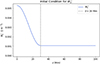 |
Fig. 1. Initial profile of outward propagating kink wave energy as a function of height over the 100 Mm domain. Beyond 30 Mm, the initial wave energy is assumed to be constant. |
3.3. Simulation comparison
Results obtained from both the Python and MPI-AMRVAC simulations of outwardly propagating kink wave energy, temperature, velocity, and density over the same time span and setup are compared in Figure 2. In these simulations, the Alfvén wave energy is set to zero to isolate the evolution of kink wave energy and its impact on the coronal plasma.
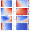 |
Fig. 2. Results obtained from the new module UAWSoM in MPI-AMRVAC shown from top to bottom for: the outward propagating kink wave energy (J m−3), temperature (MK), the velocity (km s−1), and the plasma density (kg m−3) as functions of time (seconds) and space, z (Mm). The left-hand column represents the results obtained from the MPI-AMRVAC implementation of UAWSoM, while the data presented in the right-hand column were obtained from the Python implementation. |
The observed differences are primarily attributed to variations in how identical boundary conditions are implemented. Specifically, MPI-AMRVAC uses ghost cells to extrapolate physical quantities beyond the domain, whereas the Python version lacks this capability. This means that MPI-AMRVAC can properly account for energy outside of the domain, resulting in stable inflows. Furthermore, MPI-AMRVAC has adaptive time-stepping, which helps manage steep gradients during the relaxation phase (a feature not present in the Python implementation). Differences in how thermal conduction and radiative losses are treated also contribute to the discrepancies. However, after extensive testing (not shown), including runs without radiative losses and/or thermal conduction, we conclude that boundary condition treatment is the dominant factor. The goal here is not to assess the Python code, but to validate the results of Van Doorsselaere et al. (2025), prior to further development of the current MPI-AMRVAC module.
Due to this variation in boundary behaviour, the two simulations exhibit variation in the flow of plasma, resulting in differing levels of adiabatic heating and/or cooling. Adiabatic heating and cooling processes are likely to account for the majority of discrepancies observed between the two simulations’ results. In the MPI-AMRVAC simulations, condensations develop in the lower half of the domain, resulting in downflows, while wave pressure is significant enough to induce upflows in the upper half of the domain. This dispersion of mass leads to additional cooling effects beyond those attributable to radiative losses. In contrast, the Python-based simulations exhibit strong upflows entering from the lower boundary, with an effect on the outcome of the simulation. These upflows are not correspondingly balanced at the upper boundary; this is an inconsistency that becomes significant when considering the stratified nature of the plasma.
Despite these differences in dynamics, both simulations display broadly similar temperature profiles, suggesting the dominant heating mechanism remains kink wave heating. Plasma cooling is most pronounced near the base of the domain, where the density is greatest, while temperatures at the top boundary exceed the initial uniform temperature of 1 MK.
3.4. Steady state UAWSoM solution
One of the fundamental questions we answer in this study relates to whether we can maintain a stable model atmosphere without anomalous background heating. Below, we present an approach to answering this question. A stable atmosphere without background heating that exhibits coronal temperatures that are maintained against radiative losses solely by kink wave heating. The straight contour lines in Figure 3 show that the system has reached a steady state. To obtain the results in Figure 3, we simply needed to run the above simulation for longer.
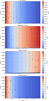 |
Fig. 3. MPI-AMRVAC simulation as prescribed in Figure 2, but now the simulation is allowed to run for much longer. We considered this to be a quasi-steady state. The quantities shown are the outward propagating kink wave energy (J m−3), temperature (MK), the velocity (in km s−1), and the plasma density (kg m−3) as functions of time (seconds) and space, z (Mm). |
The solar corona is an optically thin plasma and is characterised by a typical temperature of T ≈ 106 K and number density of n ≈ 1015 m−3. These conditions correspond to an internal energy density of approximately e ∼ 2 × 10⁻² J m−3. The associated optically thin radiative loss rate is on the order of Qrad ∼ 10−5 W m−3, yielding a characteristic radiative cooling timescale of
which is typically the longest relevant physical timescale in the coronal plasma. Our temporally extended simulation (presented in Figure 3) was run over timescales that are much longer than any of these characteristic values, ensuring that the system has sufficient time to evolve dynamically and thermodynamically. This allows for a proper investigation of quasi-steady-state coronal configurations and wave heating processes.
As Figure 3 demonstrates, the kink wave heating is entirely responsible for maintaining coronal plasma temperatures ∼1 MK. The steady outflow at the top boundary is balanced by a steady inflow (as shown in the constant density and velocity profile in time), suggesting there is negligible adiabatic heating occurring in our simulation. Satisfied with the implementations of the set of governing equations within the MPI-AMRVAC framework, we now present a collection of results obtained through a parameter study of the various user-defined variables.
4. Parameter study: varied Alfvén wave reflection rates
In the previously discussed AWSoM models, it is a necessity that the equations produce a source of reflected Alfvén waves. There is some variation in the literature on what this reflection should be. For example, Réville et al. (2020) used a constant reflection rate of 0.1, while van der Holst et al. (2014) used a more involved function involving the curl of the velocity field and the gradient of the Alfvén speed. Downs et al. (2016) used a simpler reflection rate dependent on the gradient of the Alfvén speed, which can be obtained by considering the one-dimensional case of van der Holst et al. (2014), where the curl of the velocity field is naturally zero. This term is analogous to the work of Heinemann & Olbert (1980) who calculated the non-Wentzel–Kramers–Brillouin (WKB) reflection rate in a stratified plasma, only now Downs et al. (2016) ignored the effect of the radial acceleration of the wind on reflection. When the equations are written in terms of wave energy, van der Holst et al. (2014) and Downs et al. (2016) require a ‘seed’ of inward propagating wave energy for reflection to occur, since the terms corresponding to reflection contain both inward and outward propagating wave energy. This means that unidirectionally propagating wave energy does not self-consistently produce a source of counterpropagating wave energy, which is a result of the parameterisation of the wave energy necessary to run global models. It is not our goal to reproduce the results previously obtained, but, rather, to offer supporting evidence of the relative capabilities of Alfvén and kink waves to heat a coronal plasma. For this reason, we chose a reflection rate that can produce reflected waves in a self-consistent way without the requirement of initial wave energy propagating in both directions. We took inspiration from the aforementioned literature, along with the reflection term we consider in Equation (5), given by
 (34)
(34)
where σ is a constant that we vary between simulations to simulate stronger or weaker Alfvén wave energy reflection. The quantity in the brackets reflects the importance of the background flow on reflection, which was derived from Downs et al. (2016). The approach we took involved allowing σ to be a free parameter, similar to that taken by Matthaeus et al. (1999) and Chandran & Hollweg (2009), who conducted parameter studies where the reflection rate was varied between simulations. This approach aims to quantify the significance of an Alfvén speed gradient on the reflection of Alfvén wave energy. Varying σ is motivated by assuming varied frequency compositions of the wave energy and the impact this would have on reflection (Soler 2025). This places more or less emphasis on Alfvén wave heating as the dominant contributing factor to the overall plasma heating and can shift the distribution of heating within the domain.
4.1. Simulation results
Below, Figures 4 and 5 show the temperature and velocity profiles as functions of height and the Alfvén wave and kink wave heating contributions, respectively. The values of σ inserted into the reflection function given by Equation (34), are given by σ = 0 (black), 0.1 (blue), 0.2 (green), 0.5 (orange), 1 (red), and 5 (pink). For these simulations, we considered the energy injections of the two waves to be initially identical and exactly one-half of the value employed in Section 3. As a result, the sum of the two wave energy injections at the base of the domain achieves the value given by Wk0. The initial energy injection is supplemented by an identical injection at the base (i.e., while the damping profiles of the two waves can vary, their base injection remains the same throughout the simulation). Given the same energy input, kink waves and Alfvén waves do not have the same heating rates; the kink wave heating term is proportional to the kink wave energy to the power of three halves, while the heating due to Alfvén waves is proportional to one of the inward or outward propagating Alfvén wave energies multiplied by the other signed Alfvén wave energy to the power of one-half. Given the similarity between the correlation length scales for kink waves and Alfvén waves, at least in the lower atmosphere (typically of the order of a few percent of a R⊙), we can simplify the forthcoming explanation of the disparity in heating rates by neglecting the impact of differing dissipation lengths. The reason for the discrepancies then comes from the condition that Alfvén waves can only heat the plasma if both inward and outward propagating waves coexist at the same spatial position. Throughout the present study, we consider that inward propagating Alfvén wave energy can only be generated through the reflection of Alfvén wave energy that originated as outwardly propagating Alfvén wave energy. In the limit of full Alfvén wave reflection, all of WA− can be fed into WA+, resulting in the heating rates for Alfvén and kink waves matching at this infinitesimally small reflective point, provided this point is the first and only location of reflection within the domain. In every case less extreme than full reflection, Alfvén wave heating is strictly less efficient than kink wave heating at every spatial point, thus highlighting the efficiency of uniturbulent dissipation in heating the structured solar atmosphere; this is especially valid in weakly stratified plasmas, where reflection is minimal.
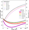 |
Fig. 4. Temperature (in MK given by various line styles and colors) and velocity (in km s−1 given by various thickness and color solid lines) are given as a function of height (Mm) plotted at time t = 1800 s, where the reflection coefficient (σ) corresponding to Alfvén wave energy reflection is varied. The reflection coefficients (σ) are 5 (pink), 1 (red), 0.5 (orange), 0.2 (green), 0.1 (blue), and 0 (black) which leads to no Alfvén wave heating. The various thicknesses of lines refer to the velocity and the various line styles refer to the temperature. |
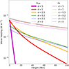 |
Fig. 5. Heating rates (given in W m−3) corresponding to Alfvén and kink waves given the same energy injection are shown as functions of height for the various reflection rates considered. The reflection coefficients (σ) are 5 (pink), 1 (red), 0.5 (orange), 0.2 (green), 0.1 (blue), and 0 (black) which leads to no Alfvén wave heating. The various thicknesses of lines refer to the Alfvén wave heating term, and the various line styles refer to the kink wave heating terms. |
The discrepancies in the heating rates explain why Figure 4 exhibits only minor variations in temperature as we vary the Alfvén wave energy reflection rate; the dominant heating contribution remains associated with kink waves. In Figure 5, only in the case of exceptionally strong reflection (σ = 5, pink line) does the Alfvén wave heating approach the magnitude of the kink wave heating near the lower boundary. It is important to note, however, that even in this extreme scenario, Alfvén wave heating in the upper atmosphere remains negligible. Furthermore, the enhanced downward-propagating Alfvén wave energy associated with strong reflection introduces a destabilising influence on the atmosphere (not associated with a lack of wave energy, but, rather, an excess of localised wave pressure), ultimately leading to catastrophic cooling. This is the reason we present results at t = 1800 s and cannot extend the simulation beyond this time. We note that while Alfvén and kink wave heating do not directly interact with one another, the influence that each wave has on plasma quantities (e.g., density) results in the kink wave heating differing from one simulation to the other. This is shown in Figure 5, specifically, in the variation in the kink wave heating profile, Qk.
4.2. Increased Alfvén wave injection
Due to this inefficiency in Alfvén wave heating, we chose to increase the Alfvén wave energy injection at the base of the domain, such that the heating rates for Alfvén and kink waves are comparable. To select this value, we calculated an approximate efficiency ratio between Alfvén and kink waves. The heating rate corresponding to Alfvén waves,  and since inward propagating Alfvén wave energy, WA+ is generated solely within the domain through the reflection (and consequent depletion) of inward propagating Alfvén wave energy, WA−, it is possible to rewrite the heating rate in terms of outward propagating Alfvén wave energy, only. We can therefore express the heating rate in terms of a function of one variable that achieves its maximum when the total Alfvén wave energy is partitioned into a ratio of 2 : 1. By assigning wave energy according to this ratio, we can derive an efficiency ratio between Alfvén and kink wave heating to be
  . This factor indicates that, even under conditions of optimal reflection, the Alfvén wave heating rate would be just over one-third of that of the kink wave, assuming equal total energy content. It should be noted that in practice the integrated Alfvén wave energy is not equal to the kink wave energy, as reflection tends to retain Alfvén wave energy within the domain for a larger amount of time. Taking this into account, these calculations provide Alfvén waves with every opportunity to outperform kink waves.
We now conduct similar simulations to Section 4.1 whereby we keep the energy injections the same between simulations (with the increased Alfvén wave energy injection), and vary our reflection coefficient, σ. Figures 6 and 7 present the temperature and velocity profiles and the heating components of Alfvén waves and kink waves as a function of height, respectively, at t = 1800 s.


We find that there is an optimum reflection coefficient to generate the highest temperature plasma that relates to the green line (σ = 0.2) in Figure 6. In addition, we once again find that extreme levels of reflection (for σ = 5, represented by the pink line) cause an unstable influence on the plasma. Here, the Alfvén wave energy is concentrated around the base of the domain and disrupts the stability of the atmosphere, resulting in catastrophic cooling of the plasma. As discussed, Alfvén waves have a lower efficiency compared to kink waves in terms of their ability to heat a plasma; in addition, it has been shown that a corresponding increase in their energy injection cannot account for this inefficiency.
5. Parameter study: varied Alfvén to kink energy
In this section, we fixed the constant, σ, used in defining the reflection rate for Alfvén waves and varied the injected Alfvén and kink wave energy ratio at the base of the domain, such that the total energy injection at the base of the domain is equal throughout all simulations. We could argue that due to reflection, the cases where more Alfvén wave energy is considered, the energy remains in the system for longer before propagating out of the open boundaries, allowing the Alfvén wave energy more time to heat the plasma. However, until an accurate reflection rate for kink waves is obtained, we cannot mitigate this effect; instead, we can simply bear it in mind. We settled on a value of σ = 0.5 for the reflection coefficient of Alfvén waves since this value is consistent with the aforementioned literature. That being said, we went on to conduct a parameter study where we varied the relative energy injection of the Alfvén and kink waves present in our simulation.
Each line in Figure 8 represents a different ratio of Alfvén to kink wave energy. Red represents a simulation with only kink wave heating, orange represents a simulation with identical total energy, but now spread across Alfvén and kink wave energy. As a result, there is three times as much kink wave energy as Alfvén wave energy (3:1 ratio). Here, the green line represents a balanced input of Alfvén and kink wave energy (1:1), the blue line represents a simulation where the Alfvén wave energy is dominant over kink wave energy (1:3 ratio), and, lastly, the black line represents a simulation with only Alfvén wave energy. Below, Figures 8 and 9 show the temperature and velocity and the relative heating rates for each wave component as a function of height, respectively.
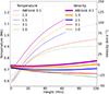 |
Fig. 8. Temperature and velocity are shown as functions of height (Mm) plotted at a time of t = 1800 s, where the ratio of Alfvén to kink wave energy is varied. The various ratios (Alfvén : kink) are 0:1 (pink), 1:3 (orange), 1:1 (blue), 3:1 (red), and 1:0 (green). The various thicknesses of the lines refer to the velocity and the various line styles refer to the temperature. |
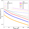 |
Fig. 9. Heating rates corresponding to Alfvén and kink waves shown as functions of height for the Alfvén-to-kink-wave energy ratios. The various ratios (Alfvén : kink) are 0:1 (pink), 1:3 (orange), 1:1 (blue), 3:1 (red), and 1:0 (green). The various thicknesses of the lines refer to the Alfvén wave heating term and the various line styles refer to kink wave heating terms. |
Previously, we mentioned that Alfvén waves alone cannot maintain an open field coronal plasma without the inclusion of an anomalous background heating function. This is why in Figures 8 and 9, we consider times before catastrophic cooling has had time to take effect. The Alfvén waves alone do not heat the atmosphere sufficiently, resulting in condensations (within the domain) with net inflow (negative) velocities. This considerable inflow causes the mass to drain out of the upper atmosphere, causing a collection of mass at the bottom boundary that cools catastrophically because the wave heating cannot compensate for the increased radiative losses.
Throughout Sections 4 and 5, we demonstrated that the wave heating rates fall below the predicted value of the radiative losses of the solar corona at 1 MK (10−5 W m−3). This explains why the lower regions of our atmosphere exhibit lower temperatures. However, near the upper boundary (where the density has reduced significantly), we find the radiative losses decrease to approximately 10−7 W m−3. The kink wave heating rates in these regions exceed these lower losses, which helps maintain stable heating and allows the solar atmosphere to reach equilibrium.
6. Open field evolution: 1-3 R⊙
Having demonstrated that wave heating can efficiently sustain an atmosphere extending up to 100 Mm, it is natural to ask whether the same mechanism can operate on even larger scales. In particular, the solar corona itself extends far beyond 100 Mm, and understanding the mechanisms that maintain its high temperatures out to distances comparable to the solar radius remains a central challenge in solar physics. In this section, we extend our model to investigate wave heating in an atmosphere reaching 3 R⊙. Due to the extended atmosphere, we have to reduce the initial wave energy profile presented in Figure 1 at large altitudes in the domain through the use of an exponential function. In addition, our domain now greatly exceeds the predicted length scale of gravity in the solar atmosphere; hence, we needed to consider it to also vary with height. This assumption alters our boundary conditions in that gravity now varies between the upper and lower boundaries, while the remaining changes are given below:
 (35)
(35)
 (36)
(36)
 (37)
(37)
where Wk0 = 5.3 × 10⁻³ J m−3 and the scale height of 20 Mm refers to the exponential. The choice of profile for the initial wave energy in the domain is arbitrary, but it is sufficient to allow the code to run stably.
In Figure 10, we chose to showcase the stable atmosphere maintained by kink waves alone, since this setup provided the most stable atmosphere. It optimally showcases the efficiency of kink wave heating through uniturbulence.
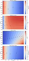 |
Fig. 10. MPI-AMRVAC simulation as prescribed in Equations (37). We consider this a quasi-steady state. The quantities shown are the outward propagating kink wave energy scaled by log10 (J m−3), temperature (MK), plasma velocity (km s−1), and the plasma density scaled by log10 (kg m−3), as functions of time (seconds) and space, z (Mm). |
In our simulations, it is necessary to evolve the system for a sufficient duration to ensure that artefacts arising from the initial conditions are advected out of the computational domain, often in the form of a shock wave. To avoid confusion with these transient events, we present our results after this shock has propagated beyond the domain boundaries. We focus instead on the (quasi-)steady state that subsequently develops. Notably, this initial shock does not arise in simulations with the smaller domain size. We attribute this to the lower densities and pressures characteristic of the larger domain setup. Additionally, during the advection of the shock wave, the larger domain exhibits a net mass outflow (a feature that is far less pronounced in the smaller domain), which leads to a modified steady-state compared to the smaller domain. Since the rate of the wave energy injection is constant across all simulations, the differences in mass retained in each domain can lead to differences in temperatures and outflow velocities. Thermal conduction redistributes this heating throughout the domain, leading to global differences in the temperature profile. That said, comparing Figures 10 and 3, the temperature at the top boundary matches the temperature at 100 Mm in the much larger 1–3 R⊙ simulation very well, suggesting that these discrepancies have only a minor effect on the overall solution.
7. Notes on the UAWSoM model
In this investigation, we have made some general simplifications to make progress and improve upon the widely used AWSoM model. In this section, we address the potential impacts these assumptions may have on the model.
7.1. Reflection rates for kink waves
In this work, we omitted the study of the reflection of kink waves. There has been, to the best of our knowledge, no investigation that has successfully quantified the reflection a kink wave undergoes due to atmospheric stratification. That being said, kink waves do not require counterpropagating waves to heat the plasma, as they undergo self-cascade via uniturbulence. Therefore, in the current setup, any reflection of kink waves will only work to redistribute the location of heating, rather than guarantee it, as is the case for Alfvén waves. If kink wave reflection were to be modeled analogously to Alfvén wave energy reflection, making it proportional to the longitudinal gradient in wave speed, it would likely concentrate heating in the lower regions of the atmosphere, where gradients in the magnetic field and density are steepest. This, in turn, would most likely yield a temperature profile that is closer to being isothermal than the steady state shown in Figures 3 and 10. This was also observed by Aschwanden et al. (2000), who found EUV loops that consist of near-isothermal threads with a substantially smaller temperature gradient than is predicted by the Rosner-Tucker-Vaiana scaling law model with gravitational stratification incorporated (Rosner et al. 1978; Serio et al. 1981, known as the RTVS scaling law).
In addition to kink wave reflection, it is also likely that Alfvén and kink waves will interact with themselves, as well as with one another nonlinearly (in the case of self-interaction of Alfvén waves, we have already taken into account), resulting in the expedition of the dissipation of wave energy. This was shown by Guo et al. (2019), where Alfvén and kink waves, when in the presence of one another, expedited the onset of the Kelvin-Helmholtz instability. In our simulations, this could be quantified by introducing a new correlation length for kink waves that have been coupled to Alfvén waves (e.g., L⊥, k, AW), which may multiply term(s) proportional to some power and combination of Wk± and WA∓. It is also likely that the relative power in the Alfvén and kink waves would play a role in this dissipation length. This is also beyond the scope of the present study, however, we aim to address these coupling effects in a future study. In the present investigation, we instead focus on the separate roles that kink waves and Alfvén waves have on the atmosphere.
7.2. Resonant absorption
In our model, we considered a density inhomogeneity represented by a discontinuity with a given magnitude, ζ. Discontinuities are a mathematical simplification and clearly do not exist in the solar atmosphere; thus, they should be replaced by a density gradient. In this case, there exists a gradient in the Alfvén speed, which can lead to resonances, resulting in the transfer of energy from the global kink mode into torsional Alfvén waves in the resonant layer. These Alfvén waves are subject to phase mixing and/or turbulent dissipation. To quantify the proportion of kink wave energy transferred to Alfvén waves and that which is available for uniturbulent dissipation, it is useful to calculate the time scales of these two processes. Van Doorsselaere et al. (2020) calculated the time scale of uniturbulence (τU) to be
 (38)
(38)
where R is the radius of the plume (or coronal loop in their case), V is the velocity amplitude of the oscillation. The time scale of resonant absorption (τRA) is given by, for instance, Goossens et al. (1992), Ruderman & Roberts (2002) as
 (39)
(39)
where l is the width of the resonant layer and P is the period of the oscillation. We note that the formulae have been adapted to match the notation consistent with the present investigation.
Given the plasma parameters employed throughout this investigation, we find that τU ≈ 12 000/V s, and τRA ≈ 1000P/l s. Given a velocity amplitude of 10 km s−1, a period of 400 s (Van Doorsselaere et al. 2020) and resonant layer 100 km in width (satisfying the condition l/R ≪ 1, Goossens et al. 1992), the two time scales are given by τU ≈ 1200 s and τRA ≈ 3800 s. This suggests that uniturbulence is a faster acting mechanism than resonant absorption, with only a relatively small amount of kink wave energy being deposited in the resonant layer in the form of Alfvén waves before uniturbulence dissipates the kink wave energy. We should preface that these calculations were done assuming a coronal loop geometry, rather than open field lines; however, we propose that uniturbulence would remain the dominant dissipation mechanism. In a future study, we intend to parameterise this transfer of energy from the kink wave to the Alfvén wave to capture this effect.
8. Conclusions and future outlook
In this study, we have extended previous wave-based coronal heating models by implementing a new physics module into the MPI-AMRVAC framework. This module includes both Alfvén and kink wave dynamics within an MHD framework. Unlike traditional models driven by Alfvén waves alone, which require an ad hoc background heating term to maintain coronal stability, our kink wave-driven simulations demonstrate that a stable 1D model atmosphere can be sustained purely through kink wave dissipation. This highlights the inherent efficiency of uniturbulent dissipation as a heating mechanism, particularly in the lower solar atmosphere, where transverse density gradients persist, enhancing the damping of kink waves.
Furthermore, we find that Alfvén waves alone are insufficient to maintain stability in our model, irrespective of the magnitude of the reflected component. In fact, under conditions of strong reflection, Alfvén waves introduce an additional destabilising influence, resulting in the onset of catastrophic cooling. In contrast, kink waves provide a more robust source of heating, capable of operating in the absence of counterpropagating wave components. Our results suggest that a hybrid model involving both Alfvén and kink waves can be viable, but only if sufficient kink wave energy is present to compensate for the limitations of Alfvén wave heating. We propose that it is likely that kink wave heating is essential in a self-consistent AC-heated corona. These findings offer a potential physical explanation for the ad hoc background heating functions often employed in AWSoM-type models (Réville et al. 2020).
We now wish to acknowledge some limitations of the modelling performed in this investigation. The base magnetic field and density contrast that were chosen are larger than estimated in the quiet Sun and coronal holes (e.g., see Morton et al. 2021), but allow for a stable atmosphere to be found. In addition, we have not included additional cooling contributions, such as strong thermal conduction down to a cooler transition region and chromosphere, as this would lead to enhanced cooling at the footpoint from transition region material. We intend to include these additional effects in future studies. In addition to these limitations, the inclusion of more complex wave modes is essential in coronal heating and solar wind driving. Future studies will include the exploration of additional wave modes, such as the slow-mode wave and their coupling to parametric instabilities (see, e.g., Shoda et al. 2018, 2019), further enhancing the realism and completeness of wave-based solar atmospheric models. In addition, as shown by Guo et al. (2019), kink waves and Alfvén waves do interact nonlinearly, leading to an earlier onset of the Kelvin-Helmholtz instability, and this is likely to play a role in reducing the correlation lengths of both wave modes, leading to stronger heating.
Building on our current advancements, we propose extending our modeling efforts to global 3D simulations of the solar atmosphere, initiated from observed magnetograms. Using field-line extrapolation techniques, such as the potential field source surface (PFSS) model, we plan to reconstruct the large-scale magnetic structure extending from the photosphere into the corona. This approach will allow us to naturally incorporate both open field regions (e.g., coronal holes) and closed magnetic loops (e.g., active regions and quiet Sun structures) into our simulations.
We aim to systematically investigate the heating of both active regions and quiet Sun areas, testing whether the turbulent cascade of kink wave energy can account for the varied thermal structures observed across the solar corona. To bridge simulation results with observations, we also plan to employ forward modeling techniques using tools such as FoMo (Van Doorsselaere et al. 2016) to synthesise observable quantities (e.g., intensity maps, Doppler shifts, line broadening) from our simulation outputs. This will enable direct comparisons with data from instruments such as SDO/AIA, Hinode/EIS, and Solar Orbiter/SPICE. We expect these global simulations will provide a powerful test of whether kink-wave-turbulence, when combined with realistic magnetic topologies, can consistently heat the solar atmosphere and drive the solar wind across a range of solar conditions.
We can use the same approach as for the Sun to model stellar atmospheres and winds of low-mass stars, as they share similar characteristics. A recent study by Vidotto et al. (2023) demonstrated the importance of using global magnetically-driven 3D models such as AWSoM to model the stellar wind (in this case around a cool dwarf) and its interaction with the orbiting exoplanet. However, the uncertainties related to the input parameters and the corresponding output, such as predicted mass-loss rate, are still large. We believe that the UAWSoM model presented here can shed more light on the stellar wind characteristics and star-planet interactions.
Acknowledgments
MM, TVD, and LB received financial support from the Flemish Government under the long-term structural Methusalem funding program, project SOUL: Stellar evolution in full glory, grant METH/24/012 at KU Leuven. Furthermore, TVD and DL were supported by a Senior Research Project (G088021N) of the FWO Vlaanderen. The research that led to these results was subsidised by the Belgian Federal Science Policy Office through the contract B2/223/P1/CLOSE-UP. It is also part of the DynaSun project and has thus received funding under the Horizon Europe programme of the European Union under grant agreement (no. 101131534). Views and opinions expressed are, however, those of the author(s) only and do not necessarily reflect those of the European Union and therefore the European Union cannot be held responsible for them.
References
- Alfvén, H. 1942, Nature, 150, 405 [Google Scholar]
- Alfvén, H. 1947, MNRAS, 107, 211 [CrossRef] [Google Scholar]
- Aschwanden, M. J., Nightingale, R. W., & Alexander, D. 2000, ApJ, 541, 1059 [NASA ADS] [CrossRef] [Google Scholar]
- Beck, C., Khomenko, E., Rezaei, R., & Collados, M. 2009, A&A, 507, 453 [NASA ADS] [CrossRef] [EDP Sciences] [Google Scholar]
- Beck, C., Rezaei, R., & Puschmann, K. G. 2012, A&A, 544, A46 [NASA ADS] [CrossRef] [EDP Sciences] [Google Scholar]
- Braginskii, S. I. 1965, Rev. Plasma Phys., 1, 205 [Google Scholar]
- Chandran, B. D. G., & Hollweg, J. V. 2009, ApJ, 707, 1659 [Google Scholar]
- Chandran, B. D. G., Dennis, T. J., Quataert, E., & Bale, S. D. 2011, ApJ, 743, 197 [Google Scholar]
- Colgan, J., Abdallah, J., Jr, Sherrill, M. E., et al. 2008, ApJ, 689, 585 [NASA ADS] [CrossRef] [Google Scholar]
- Cranmer, S. R., van Ballegooijen, A. A., & Edgar, R. J. 2007, ApJS, 171, 520 [Google Scholar]
- DeForest, C. E., Howard, R. A., Velli, M., Viall, N., & Vourlidas, A. 2018, ApJ, 862, 18 [Google Scholar]
- Downs, C., Lionello, R., Mikić, Z., Linker, J. A., & Velli, M. 2016, ApJ, 832, 180 [Google Scholar]
- Elsasser, W. M. 1950, Phys. Rev., 79, 183 [Google Scholar]
- Evans, R. M., Opher, M., Oran, R., et al. 2012, ApJ, 756, 155 [NASA ADS] [CrossRef] [Google Scholar]
- Goossens, M., Hollweg, J. V., & Sakurai, T. 1992, Sol. Phys., 138, 233 [Google Scholar]
- Goossens, M. L., Arregui, I., & Van Doorsselaere, T. 2019, Front. Astron. Space Sci., 6, 20 [Google Scholar]
- Guo, M., Van Doorsselaere, T., Karampelas, K., et al. 2019, ApJ, 870, 55 [Google Scholar]
- Guyer, J. E., Wheeler, D., & Warren, J. A. 2009, Comput. Sci. Eng., 11, 6 [NASA ADS] [CrossRef] [Google Scholar]
- Heinemann, M., & Olbert, S. 1980, J. Geophys. Res., 85, 1311 [Google Scholar]
- Hermans, J., & Keppens, R. 2021, A&A, 655, A36 [NASA ADS] [CrossRef] [EDP Sciences] [Google Scholar]
- Heyvaerts, J., & Priest, E. R. 1983, A&A, 117, 220 [NASA ADS] [Google Scholar]
- Keppens, R., Popescu Braileanu, B., Zhou, Y., et al. 2023, A&A, 673, A66 [NASA ADS] [CrossRef] [EDP Sciences] [Google Scholar]
- Lionello, R., Velli, M., Downs, C., et al. 2014, ApJ, 784, 120 [Google Scholar]
- Magyar, N., Van Doorsselaere, T., & Goossens, M. 2019, ApJ, 882, 50 [Google Scholar]
- Matthaeus, W. H., Zank, G. P., Oughton, S., Mullan, D. J., & Dmitruk, P. 1999, ApJ, 523, L93 [NASA ADS] [CrossRef] [Google Scholar]
- McMurdo, M., Ballai, I., Verth, G., Alharbi, A., & Fedun, V. 2023, ApJ, 958, 81 [NASA ADS] [CrossRef] [Google Scholar]
- McMurdo, M., Ballai, I., Verth, G., & Fedun, V. 2025, ApJ, 988, 50 [Google Scholar]
- Mikić, Z., Downs, C., Linker, J. A., et al. 2018, Nat. Astron., 2, 913 [Google Scholar]
- Morton, R. J., & Cunningham, R. 2023, ApJ, 954, 90 [NASA ADS] [CrossRef] [Google Scholar]
- Morton, R. J., Tomczyk, S., & Pinto, R. 2015, Nat. Commun., 6, 7813 [Google Scholar]
- Morton, R. J., Tomczyk, S., & Pinto, R. F. 2016, ApJ, 828, 89 [Google Scholar]
- Morton, R. J., Tiwari, A. K., Van Doorsselaere, T., & McLaughlin, J. A. 2021, ApJ, 923, 225 [NASA ADS] [CrossRef] [Google Scholar]
- Pelouze, G., Van Doorsselaere, T., Karampelas, K., Riedl, J. M., & Duckenfield, T. 2023, A&A, 672, A105 [NASA ADS] [CrossRef] [EDP Sciences] [Google Scholar]
- Raymond, J. C., McCauley, P. I., Cranmer, S. R., & Downs, C. 2014, ApJ, 788, 152 [NASA ADS] [CrossRef] [Google Scholar]
- Réville, V., Velli, M., Panasenco, O., et al. 2020, ApJS, 246, 24 [Google Scholar]
- Riley, P., Downs, C., Linker, J. A., et al. 2019, ApJ, 874, L15 [Google Scholar]
- Roberts, B. 1981, in The Physics of Sunspots, eds. L. E. Cram, & J. H. Thomas, 369 [Google Scholar]
- Rosner, R., Tucker, W. H., & Vaiana, G. S. 1978, ApJ, 220, 643 [Google Scholar]
- Ruderman, M. S., & Roberts, B. 2002, ApJ, 577, 475 [Google Scholar]
- Serio, S., Peres, G., Vaiana, G. S., Golub, L., & Rosner, R. 1981, ApJ, 243, 288 [NASA ADS] [CrossRef] [Google Scholar]
- Sharma, R., & Morton, R. J. 2023, Nat. Astron., 7, 1301 [CrossRef] [Google Scholar]
- Shoda, M., Yokoyama, T., & Suzuki, T. K. 2018, ApJ, 853, 190 [Google Scholar]
- Shoda, M., Suzuki, T. K., Asgari-Targhi, M., & Yokoyama, T. 2019, ApJ, 880, L2 [Google Scholar]
- Soler, R. 2025, ApJ, 985, 95 [Google Scholar]
- Soler, R., & Terradas, J. 2015, ApJ, 803, 43 [Google Scholar]
- Stenborg, G., Howard, R. A., Hess, P., & Gallagher, B. 2021, A&A, 650, A28 [EDP Sciences] [Google Scholar]
- Suzuki, T. K., & Inutsuka, S.-I. 2005, ApJ, 632, L49 [NASA ADS] [CrossRef] [Google Scholar]
- Suzuki, T. K., & Inutsuka, S.-I. 2006, J. Geophys. Res. (Space Phys.), 111, A06101 [Google Scholar]
- Tomczyk, S., McIntosh, S. W., Keil, S. L., et al. 2007, Science, 317, 1192 [Google Scholar]
- Uritsky, V. M., DeForest, C. E., Karpen, J. T., et al. 2021, ApJ, 907, 1 [NASA ADS] [CrossRef] [Google Scholar]
- van Ballegooijen, A. A., Asgari-Targhi, M., Cranmer, S. R., & DeLuca, E. E. 2011, ApJ, 736, 3 [Google Scholar]
- van der Holst, B., Sokolov, I. V., Meng, X., et al. 2014, ApJ, 782, 81 [Google Scholar]
- Van Doorsselaere, T., Gijsen, S. E., Andries, J., & Verth, G. 2014, ApJ, 795, 18 [NASA ADS] [CrossRef] [Google Scholar]
- Van Doorsselaere, T., Antolin, P., Yuan, D., Reznikova, V., & Magyar, N. 2016, Front. Astron. Space Sci., 3, 4 [Google Scholar]
- Van Doorsselaere, T., Li, B., Goossens, M., Hnat, B., & Magyar, N. 2020, ApJ, 899, 100 [NASA ADS] [CrossRef] [Google Scholar]
- Van Doorsselaere, T., Magyar, N., Sieyra, M. V., & Goossens, M. 2024, J. Plasma Phys., 90, 905900113 [Google Scholar]
- Van Doorsselaere, T., Sieyra, M. V., Magyar, N., Goossens, M., & Banović, L. 2025, A&A, 696, A166 [NASA ADS] [CrossRef] [EDP Sciences] [Google Scholar]
- Verdini, A., & Velli, M. 2007, ApJ, 662, 669 [Google Scholar]
- Verdini, A., Velli, M., Matthaeus, W. H., Oughton, S., & Dmitruk, P. 2010, ApJ, 708, L116 [Google Scholar]
- Vidotto, A. A., Bourrier, V., Fares, R., et al. 2023, A&A, 678, A152 [NASA ADS] [CrossRef] [EDP Sciences] [Google Scholar]
- Weberg, M. J., Morton, R. J., & McLaughlin, J. A. 2020, ApJ, 894, 79 [NASA ADS] [CrossRef] [Google Scholar]
- Wilhelm, K., Abbo, L., Auchère, F., et al. 2011, A&A Rev., 19, 35 [NASA ADS] [CrossRef] [Google Scholar]
- Xia, C., Teunissen, J., El Mellah, I., Chané, E., & Keppens, R. 2018, ApJS, 234, 30 [Google Scholar]
All Figures
|
Fig. 1. Initial profile of outward propagating kink wave energy as a function of height over the 100 Mm domain. Beyond 30 Mm, the initial wave energy is assumed to be constant. |
| In the text | |
|
Fig. 2. Results obtained from the new module UAWSoM in MPI-AMRVAC shown from top to bottom for: the outward propagating kink wave energy (J m−3), temperature (MK), the velocity (km s−1), and the plasma density (kg m−3) as functions of time (seconds) and space, z (Mm). The left-hand column represents the results obtained from the MPI-AMRVAC implementation of UAWSoM, while the data presented in the right-hand column were obtained from the Python implementation. |
| In the text | |
|
Fig. 3. MPI-AMRVAC simulation as prescribed in Figure 2, but now the simulation is allowed to run for much longer. We considered this to be a quasi-steady state. The quantities shown are the outward propagating kink wave energy (J m−3), temperature (MK), the velocity (in km s−1), and the plasma density (kg m−3) as functions of time (seconds) and space, z (Mm). |
| In the text | |
|
Fig. 4. Temperature (in MK given by various line styles and colors) and velocity (in km s−1 given by various thickness and color solid lines) are given as a function of height (Mm) plotted at time t = 1800 s, where the reflection coefficient (σ) corresponding to Alfvén wave energy reflection is varied. The reflection coefficients (σ) are 5 (pink), 1 (red), 0.5 (orange), 0.2 (green), 0.1 (blue), and 0 (black) which leads to no Alfvén wave heating. The various thicknesses of lines refer to the velocity and the various line styles refer to the temperature. |
| In the text | |
|
Fig. 5. Heating rates (given in W m−3) corresponding to Alfvén and kink waves given the same energy injection are shown as functions of height for the various reflection rates considered. The reflection coefficients (σ) are 5 (pink), 1 (red), 0.5 (orange), 0.2 (green), 0.1 (blue), and 0 (black) which leads to no Alfvén wave heating. The various thicknesses of lines refer to the Alfvén wave heating term, and the various line styles refer to the kink wave heating terms. |
| In the text | |
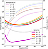 |
Fig. 6. Same setup as Figure 4, but with increased Alfvén wave energy by a factor of |
| In the text | |
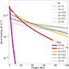 |
Fig. 7. Same setup as Figure 5, but with increased Alfvén wave energy by a factor of |
| In the text | |
|
Fig. 8. Temperature and velocity are shown as functions of height (Mm) plotted at a time of t = 1800 s, where the ratio of Alfvén to kink wave energy is varied. The various ratios (Alfvén : kink) are 0:1 (pink), 1:3 (orange), 1:1 (blue), 3:1 (red), and 1:0 (green). The various thicknesses of the lines refer to the velocity and the various line styles refer to the temperature. |
| In the text | |
|
Fig. 9. Heating rates corresponding to Alfvén and kink waves shown as functions of height for the Alfvén-to-kink-wave energy ratios. The various ratios (Alfvén : kink) are 0:1 (pink), 1:3 (orange), 1:1 (blue), 3:1 (red), and 1:0 (green). The various thicknesses of the lines refer to the Alfvén wave heating term and the various line styles refer to kink wave heating terms. |
| In the text | |
|
Fig. 10. MPI-AMRVAC simulation as prescribed in Equations (37). We consider this a quasi-steady state. The quantities shown are the outward propagating kink wave energy scaled by log10 (J m−3), temperature (MK), plasma velocity (km s−1), and the plasma density scaled by log10 (kg m−3), as functions of time (seconds) and space, z (Mm). |
| In the text | |
Current usage metrics show cumulative count of Article Views (full-text article views including HTML views, PDF and ePub downloads, according to the available data) and Abstracts Views on Vision4Press platform.
Data correspond to usage on the plateform after 2015. The current usage metrics is available 48-96 hours after online publication and is updated daily on week days.
Initial download of the metrics may take a while.