| Issue |
A&A
Volume 705, January 2026
|
|
|---|---|---|
| Article Number | A11 | |
| Number of page(s) | 10 | |
| Section | Interstellar and circumstellar matter | |
| DOI | https://doi.org/10.1051/0004-6361/202556080 | |
| Published online | 23 December 2025 | |
Stellar feedback effects on the mass distribution of clouds and cloud complexes
1
Department of Physics and Astronomy, Barnard College,
New York,
NY,
10025,
USA
2
Department of Astrophysics, American Museum of Natural History,
200 Central Park West,
New York,
NY,
10024,
USA
★ Corresponding author: This email address is being protected from spambots. You need JavaScript enabled to view it.
Received:
24
June
2025
Accepted:
21
November
2025
Abstract
Context. Galaxy evolution is sensitive to how stars inject feedback into their surroundings. In particular, the stellar feedback from star clusters strongly affects gas motions and, consequently, the baryonic cycle. More massive clusters have stronger effects. Our previous results show that the star cluster mass distribution in dwarf galaxies depends on feedback because strong pre-supernova feedback, particularly ionizing radiation, results in fewer high-mass star clusters.
Aims. We investigated the mass distribution of gas clouds in dwarf galaxies. Since star clusters form from the collapse of gas clouds, we expected similar feedback dependences in both their mass distributions; we thus hypothesized that pre-supernova feedback results in fewer high-mass gas clouds.
Methods. To test our hypothesis, we used an isocontour analysis at three cutoff densities n = 10, 101.5, and 102 cm−3 to identify gas clouds from dwarf galaxy simulations performed with the RAMSES adaptive mesh refinement code. We calculated mass distributions for models that implement different combinations of the feedback modes: supernovae, stellar winds from massive stars, and ionizing radiation.
Results. We find that the mass distribution for clouds with n > 100 cm−3 is independent of feedback, but that the mass distribution for cloud complexes with n > 10 cm−3 is more top-heavy in the presence of radiation. Winds do not affect the mass distribution at any of the scales we studied.
Conclusions. This contradicts our hypothesis that the mass distribution of gas clouds would show a similar feedback dependence as the mass distribution of star clusters. Instead, our results show no feedback dependence in the mass function of dense clouds with n > 100 cm−3, suggesting their mass distribution is predominantly set by gravity. We conclude that the shape of the star cluster mass function must be determined by a combination of intra-cloud feedback regulation of star formation (i.e., regulation of star formation within a cloud due to the feedback of stars formed from that cloud itself) and, in the case of radiation, effects on the temperature of the parent gas clouds.
Key words: methods: data analysis / methods: numerical / ISM: clouds / ISM: general / ISM: kinematics and dynamics
© The Authors 2025
 Open Access article, published by EDP Sciences, under the terms of the Creative Commons Attribution License (https://creativecommons.org/licenses/by/4.0), which permits unrestricted use, distribution, and reproduction in any medium, provided the original work is properly cited.
This article is published in open access under the Subscribe to Open model. This email address is being protected from spambots. You need JavaScript enabled to view it. to support open access publication.
1 Introduction
A longstanding question about the star formation process is the connection between star clusters and the clouds from which they emerge (Lada & Lada 2003; Dobbs et al. 2014; Krumholz et al. 2019; Chevance et al. 2023; Knutas et al. 2025; Pedrini et al. 2025). Because of the timescales involved, this question is currently impossible to address directly through observations of a single cloud evolving into a star cluster – statistical studies of populations are instead required. Star formation is often investigated through theoretical models constrained by accessible observables. For example, the depletion time, the rate at which gas is consumed by star formation, can be determined empirically by comparing the available molecular gas mass and the star formation rate. While this provides insight into the star formation process, large scatter is observed in the depletion time, particularly at small scales (Onodera et al. 2010; Schruba et al. 2010). Another property guiding our understanding of these processes is the star formation efficiency per free-fall time, which is typically observed to be low (only a few percent; Krumholz et al. 2019). However, while convenient from a modeling perspective, this property relies on the assumption that there exists a scale at which interstellar gas is converted into stars through the collapse of a single structure in free fall. In reality, the interstellar medium (ISM) is filamentary and supported by turbulence (Mac Low & Klessen 2004; McKee & Ostriker 2007; Burkhart 2018), has dynamics affected by magnetic fields (Crutcher 2012), and is affected by large-scale shear (Dobbs et al. 2014; Jeffreson et al. 2020). While it is possible to attribute the low efficiency of star formation to these factors, it might also be the case that stars indeed form from gas in free fall, and that this happens rarely but with rapid inhibition by feedback. Therefore, when viewed as an average over a larger scale, star formation appears inefficient (Semenov et al. 2017).
Rather than individual objects, populations of clusters and clouds can be analyzed; this allows the evolution to be inferred from the distribution of objects at different stages (Knutas et al. 2025). Particular attention has been drawn to the similar shape of the mass distribution of these clusters and clouds (see, e.g., Guszejnov et al. 2018). For star clusters, the mass distribution typically shows a power-law function with a steep negative slope c ≃ −2; Portegies Zwart et al. 2010; Krumholz et al. 2019; Adamo et al. 2020; Pedrini et al. 2025. Interestingly, the mass distribution for gas structures shows a similar profile (Colombo et al. 2019), although there is some dependence on environment (Rosolowsky 2005; Colombo et al. 2014; Rosolowsky et al. 2021).
A major challenge to addressing this question is the fact that clouds are part of a continuum of structures in the ISM, so individual cloud properties such as mass are hard to define (as highlighted in the review by Chevance et al. 2023). Furthermore, these properties are often derived from structures determined by different observables that can show different morphologies. For example, molecular clouds observed through CO line emission often appear as structures with well-defined boundaries, while coincident structures in dust extinction maps show connected filaments as part of larger complexes (see Chevance et al. 2023 for a detailed discussion and examples).
The goal of this work is to determine how the shape of the cloud mass distribution varies as a function of feedback in hydrodynamical simulations of galaxies. We compare the cloud mass distribution to the mass distribution of star clusters derived from the same simulations (presented in Andersson et al. 2024 and replicated in Fig. 1). Of particular interest is that different sources of feedback were included in simulations of the same galaxy and the remaining model parameters were kept the same. In this way, we address (1) how different feedback mechanisms determine the cloud mass distribution and (2) how sensitive the star cluster mass distribution is to the cloud distribution from which it originates.
Andersson et al. (2024, hereafter A24) show that, in our simulations, the star cluster mass distribution depends on feedback, transitioning from a wide function approaching a log-normal shape in the absence of feedback to a steep power-law function when sources of feedback prior to supernovae (SNe), particularly ionizing radiation, are active. Furthermore, they show that this effect is tightly linked to the timescale of the active feedback, including the details that affect this timescale, for example the main-sequence lifetime for the most massive SN progenitor assumed. We tested whether this effect comes from a similar behavior in the cloud mass distribution, or whether it is related to the formation of individual star clusters inside the clouds themselves.
We start by detailing our simulations and cloud selection algorithm in Sect. 2, which is followed by a presentation of our main results in Sect. 3. In Sect. 4 we interpret the effects of feedback on cloud and cloud complex mass distributions and briefly discuss other computational and observational data. Section 5 summarizes our work.
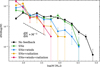 |
Fig. 1 Cluster initial mass function, normalized to the total number of clusters (defined as stellar groups with ages <25 Myr) found in each simulation after 300 Myr. The error bars indicate the 16th and 84th percentiles computed using bootstrapping. The dashed line shows the slope of scale-free formation models, often associated with the initial cluster mass function (from A24, where more details are provided). |
2 Method
2.1 Simulations
The galaxy simulations used in our analysis are described in A24. Briefly summarized, all simulations are executed with RAMSES-RT (Rosdahl et al. 2013; Rosdahl & Teyssier 2015), a radiative transfer extension of the adaptive mesh refinement and N-body code RAMSES (Teyssier 2002). Heating and cooling include the equilibrium cooling from heavy elements implemented in RAMSES, as well as nonequilibrium ionization of H and He coupled to the radiation solver following the method described in Rosdahl et al. (2013); Rosdahl & Teyssier (2015), which relies on an M1 closure for the Eddington tensor. In addition, we tracked the evolution of H2 following the method of Nickerson et al. (2018). The refinement criterion employs a quasi-Lagrangian technique aiming for approximately eight particles in each cell and cell refinement at a mass threshold of 800 M⊙. The cell size is 3.6 pc at the maximum refinement level. The simulations ran for 1000 Myr with an output cadence of 25 Myr (see A24 for visualizations of, e.g., star formation history).
The initial conditions mimic an isolated dwarf galaxy using the tool MAKEDISKGALAXY (Springel 2005). Embedded in a dark matter halo following a Navarro et al. (1997) profile is a disk with gas mass Mg,disk = 7 × 10⁷ M⊙ and stellar mass Ms,disk = 107 M⊙ and an exponential radial density profile having scale length 1.1 kpc. The gas has an initial temperature of 104 K. The initial metallicity of the gas is set to 0.1 Z⊙.
Stars and dark matter are tracked by particles of masses 100 M⊙ and 104 M⊙, respectively. Star formation proceeds by forming star particles in cells with gas density n > 103 cm−3 and temperature T < 104 K at each time step. In cells exceeding these thresholds, a discrete number of single stellar population particles, each with mass 100 M⊙, can be spawned. The number of star particles is drawn from a Poisson function with the mean number of stars given by the cell gas mass divided by a star formation rate,
![Mathematical equation: $\[\dot{\rho}_{\star}=\epsilon_{\mathrm{ff}} \frac{\rho_{\mathrm{g}}}{t_{\mathrm{ff}}},\]$](/articles/aa/full_html/2026/01/aa56080-25/aa56080-25-eq1.png) (1)
(1)
and multiplied by the timestep. We determined the star formation rate by assuming an efficiency ϵff = 0.1 per local gas free-fall time tff = [3π/(32Gρg)]1/2. When regulated by feedback, this star formation algorithm was shown to reproduce the star formation relation (Agertz & Kravtsov 2016), observed star formation efficiencies (Grisdale et al. 2019), as well as scaling relations for clouds (e.g., Larson 1981) in the Milky Way (Grisdale et al. 2018).
The stellar feedback model includes stellar winds and SNe following the method of Agertz et al. (2013), while radiation is treated through the radiative transfer method (Rosdahl et al. 2013). All feedback is calibrated assuming the initial mass distribution from Kroupa (2001). Fast stellar winds injected by massive (M* > 8 M⊙) stars are implemented as a source of momentum with a wind velocity of vw = 1000 km s−1 calibrated using STARBURST99 (Leitherer et al. 1992, 1999). Core-collapse SNe are stochastically sampled as discrete events using the main sequence lifetimes from Raiteri et al. (1996), with progenitors in the mass range M* = 8–30 M⊙, each injecting ESN = 1051 erg of energy and momentum equivalent to 12 M⊙ at a velocity of 3000 km s−1. Type Ia SNe follow the time-delay distribution of Maoz & Graur (2017) assuming a time delay of 38 Myr and rate of 2.6 × 10⁻¹³ yr−1M⊙−1. We assumed a mass loss of 1.4 M⊙ and a momentum release equivalent to ESN. Finally, radiation feedback includes scattered infrared photons (nonthermal), direct radiation pressure from optical and far-ultraviolet, Lyman-Werner radiation for H2 dissociation, and photoionizing radiation around the ionizing energies of H II, He I, and He II (bands defined as in Agertz et al. 2020).
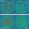 |
Fig. 2 Root node contours in projected gas density plots for different simulations (SNe in the top row, SNe+ radiation in the bottom row) and density thresholds (n > 10 cm−3 in the left column, and n > 102 cm−3 in the right column). As expected, astrodendro selects fewer and smaller structures with a higher density cutoff. |
2.2 Cloud selection
To find clouds, we first transferred the RAMSES data to a uniform grid at the maximum resolution level. We omitted data from simulation outputs in the first 300 Myr to avoid spurious effects from the initial conditions. We then employed an isocontour analysis on the density data of each simulation output using the astrodendro library (Robitaille et al. 2019) with three different density cutoffs: n > 10 cm−3, 101.5 cm−3 and 102 cm−3. We studied the properties of the largest-scale root nodes in the dendrogram for each of the three cutoffs, which we call cloud complexes, big clouds, and clouds. These choices will be discussed further in the next section, but for the moment, contrasting the right and left sides of Fig. 2 provides some visual intuition for our nomenclature. By using astrodendro for our isodensity analysis, we obtained information about cloud and cloud complex substructure that is being used to understand simulations (Wall et al. 2019, 2020) of star cluster formation from the clouds (Jiang et al., in prep).
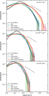 |
Fig. 3 Mass distributions for cloud complexes with n > 10 cm−3 (top), big clouds with n > 101.5 cm−3 (middle), and clouds with n > 102 cm−3 (bottom). The lines show the median values, while the shaded regions show the 16th–84th percentile range. All distributions shown contain structures from multiple snapshots, where consecutive snapshots are 25 Myr apart. The dashed line shows dN/d log(M) ∝ M−1, i.e., dN/dM ∝ M−2. |
3 Results
We focused on gas structures selected in three-dimensional space using density contours, as described in Sect. 2.2. Figure 3 shows the mass distribution obtained for different gas structures1. We note that gas in the simulation without feedback shows significantly different behavior compared with the other models, so we do not focus on it in Fig. 3, but rather on comparing the other simulations, keeping the simulation without feedback as a reference. Our mass resolution on the refined grid is under 800 M⊙, while the peaks of our mass distributions are over an order of magnitude higher, and thus probably resolved numerically.
For cloud complexes (top panel in Fig. 3), all simulations show similar fractions of low mass (M ⪅ 105 M⊙) objects. This changes at higher masses, where the mass distributions for simulations including radiation peak at a larger mass and have a shallower slope at high masses, producing a larger number of massive clouds, compared to the mass distributions for simulations without radiation. The distribution of cloud volumes behaves similarly, while the distribution of average cloud densities is mostly feedback-independent (see Appendix A). This suggests that the larger number of more massive cloud complexes formed in the presence of radiation corresponds to a larger number of larger cloud complexes. Our results thus suggest that radiation causes larger, more massive cloud complexes to form. Figure 2 illustrates this behavior – the low-density contours delineate larger, less fragmented structures when radiation is included in the simulation, a structure that remains consistent throughout the simulation.
For clouds (bottom panel in Fig. 3), the low mass end (M < 104.5 M⊙) is similar to that for the cloud complexes. However, at higher masses, the distribution function is significantly steeper. Furthermore, the cloud mass distributions in the different simulations overlap within the shown percentiles, indicating that there is insignificant feedback dependence.
For big clouds, with masses and bounding densities between cloud complexes and clouds, we see a transition where radiation plays a small role at the massive end and no role at the low mass end. This suggests an inverse proportionality between density cutoff and radiation dependence of the mass distribution, at least within the 10–100 cm−3 range.
At the massive end of the mass distribution, its slope is very steep. However, keep in mind that our mass distributions do not display a log-normal shape overall; this is consistent with other simulation studies, which tend to fit a power law only on the high-end of the spectrum (see, e.g., Renaud et al. 2024; Colman et al. 2024; Iffrig & Hennebelle 2017). More generally, the lower-mass cloud distribution with M ≲ 104.5 M⊙ remains similar regardless of density selection in all simulations, while the distribution of more massive structures more rapidly steepens when considering higher density gas.
Different simulations had different numbers of clouds, as shown in Fig. 4. In particular, adding winds and adding radiation both lead to an increase in the number of structures (clouds, big clouds, and cloud complexes) at all three density cutoffs. However, there does not seem to be a differential effect for clouds (n > 102 cm−3): the number of clouds is changed at all masses, leaving the cloud mass spectrum unchanged.
The mass distributions of clouds selected with n > 101.5 cm−3 and n > 102 cm−3 are mostly time-independent (Fig. 4), but for cloud complexes (n > 10 cm−3), the mass distribution changes with time. In particular, the difference between simulations with and without radiation at the high end of the mass distribution is more dramatic later in the simulations (see Fig. 4).
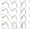 |
Fig. 4 Cloud mass distributions in 175 Myr time bins. Feedback is color-coded as in Fig. 3, and the number of clouds in each distribution is given in the legend. The lines show the median values, while the shaded regions show the 16th–84th percentile range. |
4 Discussion
4.1 Why radiation impacts the cloud complex mass function
Radiation impacts a galaxy’s gas fraction,
![Mathematical equation: $\[f_{\mathrm{gas}}=M_{\mathrm{gas}} /\left(M_{\mathrm{gas}}+M_{\mathrm{stars}}\right).\]$](/articles/aa/full_html/2026/01/aa56080-25/aa56080-25-eq2.png) (2)
(2)
Figure 5 shows the time evolution of gas fraction in the five simulations. Winds and radiation both lead to a diminished decrease in the gas fraction, although when radiation is present, the impact of adding winds is much less significant. Removal of gas through star formation alone cannot explain the evolution in gas fraction for the simulations with feedback, since star formation is higher before 600 Myr in simulations without radiation and lower after (see Fig. 2 in A24). Therefore, gas flows in and out of the disk must play a role. Radiation has been shown to decrease gas inflows and outflows (e.g., Smith et al. 2021), which appears to explain the discrepancy. A higher gas fraction leads to more gas available to form cloud complexes, which is consistent with the larger number of structures found in simulations with winds, radiation, or both (Fig. 4). However, while introducing winds simply leads to more cloud complexes, introducing radiation also changes their mass distribution, making it more top-heavy. While Renaud et al. (2024) did find that increasing gas fraction from fgas = 0.1 to 0.4 altered the shape of the clump mass distribution, they tested significantly higher changes in gas fraction without altering feedback modes, and using a different cloud extraction method (see Sect. 4.4 for details).
The thermal state of the gas plays a key role in determining the density structure. Because introducing radiation changes the balance between cooling and heating, we believe it to be responsible for the effect we find in the distribution of cloud complexes. Indeed, density-temperature phase diagrams (Fig. 6) show that introducing radiation causes the gas equilibrium curves to shift up by about 0.5 dex in temperature. The Jeans mass is proportional to temperature, so higher temperatures allow larger masses to collapse without fragmentation (Jeans 1902). This is consistent with our finding that radiation leads to higher-mass cloud complexes (Fig. 3). Furthermore, radiation leaves more mass in warm (T = 102−104 K), dense (n > 1 cm−3), high-pressure gas (Fig. 6). A24 found that radiation leads to fewer and smaller star clusters, which could also explain why cloud complexes can grow larger before being disrupted by cluster feedback. The left-hand side of Fig. 2 illustrates how radiation can reduce fragmentation in a galactic disk, resulting in more elongated cloud complexes (this is shown quantitatively by the cloud complex volume distribution in Fig. A.1). Investigating cloud lifetimes is beyond the scope of this manuscript, but should be done in future work. It is worth noting that adding radiation changes the cloud complex mass distribution significantly, even compared to removing feedback entirely. While this may seem to imply that SNe and winds do not impact the cloud complexes formed, a closer look at their volume (Fig. A.1) and density (Fig. A.2) distributions reveals that, compared to a galaxy with no feedback, one with SNe alone or SNe and winds together forms larger but less dense cloud complexes. The impact of SNe and winds thus seems to conspire in such a way as to leave the cloud complex mass function unaffected.
4.2 Mass-velocity dispersion relation
Figure 7 shows the distribution of velocity dispersion against mass for cloud complexes, big clouds, and clouds. The leftmost panel shows that galaxies with radiation have cloud complexes reaching higher masses and velocity dispersions than simulations with only SNe, winds, or both. This is consistent with the radiation dependence of the cloud complex mass function (see Sect. 3). The middle panel shows the same trend for big clouds, except that the difference is much smaller, again reflecting their mass distribution.
The rightmost panel of Fig. 7 shows that the mass-velocity dispersion relation of high mass structures is independent of the type of feedback, but that introducing a form of feedback affects this relation (cf. the simulation without any feedback). Low mass objects have slightly suppressed velocity dispersion when exposed to radiation feedback. If one interprets the velocity dispersion as a proxy for energy, it may seem surprising that feedback has so little effect. However, what we change when we add a mode of feedback is the amount of energy injected per star throughout the simulation, not necessarily the total energy budget. Our results are consistent with a self-regulating system: as the energy per star increases, the number of massive clusters decreases (A24), likely maintaining a similar total feedback budget.
Finally, the no-feedback case shows structures with a higher velocity dispersion than their counterparts of the same mass in other simulations. This effect is exacerbated at higher density cutoffs and is most prominent for clouds. The excess velocity dispersion is likely due to gravity, now unresisted by feedback (Ibáñez-Mejía et al. 2016), and more frequent collisions and mergers. This is consistent with the volume and density distributions in Figs. A.1 and A.2, which show that structures identified in the galaxy with no feedback are smaller and denser than structures in other simulations.
4.3 Feedback independence of the cloud mass function and implications
The gas cloud (n > 100 cm−3) mass distribution is feedbackindependent (Sect. 3). Feedback does affect the thermodynamics of the galaxy, as seen in Fig. 6. It also changes the number of clouds in the galaxy, but without changing the shape of the distribution, as shown in Fig. 4. This suggests the distribution of cloud masses is primarily dominated by gravity rather than feedback. A24 found that galaxies with more feedback modes had fewer massive star clusters (see Fig. 1). They showed that the formation of star clusters is sensitive to the timing of the onset of stellar feedback. As such, they concluded that the immediate regulation of local star formation provided by radiation and stellar winds prevents the most massive clusters from forming. For brevity, we call this intra-cloud feedback regulation.
The simplest competing explanation would be that the feedback dependence of the star cluster mass function is a reflection of feedback effects on the clouds from which they originate. Our results show no feedback dependence in the mass distribution of clouds, contradicting this alternative. A subtler alternative hypothesis is that feedback affects the thermodynamics or turbulence of the ISM, or both, in such a way as to prevent massive cluster formation. For clouds, although there is a dependence on the presence or absence of any feedback, all galaxies with feedback have similar velocity dispersion distributions (see Figure 7), suggesting that the impact of feedback on turbulence is also not responsible for the observed star cluster mass distributions.
Finally, the density-temperature phase diagrams in Fig. 6 show that introducing radiation causes the gas equilibrium curves to shift up by about 0.5 dex in temperature at the cold end. Radiation leads to warmer clouds with higher thermal pressure supporting against collapse, likely explaining why A24 found that including radiation resulted in fewer massive star clusters. However, while winds were found to have the same effect on the star cluster mass function (A24), they do not significantly alter the temperature of gas clouds (top left panel of Fig. 6).
Thus, through a process of elimination, we agree with the argument of A24 that intra-cloud feedback regulation of star formation leads to fewer massive clusters in galaxies with winds and radiation. However, the impact of radiation on gas cloud temperature appears to be the most important effect that we have studied.
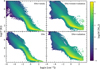 |
Fig. 6 Temperature as a function of density, color-coded by mass, for all gas in each simulation at time 750 Myr. |
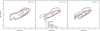 |
Fig. 7 Distribution of velocity dispersion against mass for cloud complexes (left), big clouds (center), and clouds (right). The median of the distribution is marked with a cross, while the 68th and 95th percentiles are shown as dashed and solid lines, respectively. Different models are color-coded as indicated in the legend. |
4.4 Comparison to other work
In Sect. 4.1 we discussed the results of Renaud et al. (2024) and noted that we apply a different cloud extraction method. While we used isocontours in three dimensions (see Sect. 2), they defined circular shells around gas overdensities in two-dimensional projected simulation data. Additionally, their assumed initial gas fractions are significantly lower than the initial gas fraction in our galaxy. Finally, we simulated a galaxy with a significantly lower mass compared to Renaud et al. (2024). However, the effects of feedback found in our simulations could be different in a galaxy with a different initial gas fraction. Controlling for both gas fraction and modes of feedback could shed new light on how similarly or differently the effects of feedback on cloud dynamics manifest in different galactic environments.
Renaud et al. (2024) is only one example of how other work using simulations defines clouds differently than we do. Other cloud extraction algorithms include friends-of-friends, which dictates that two particles or grid cells with a density above the required threshold belong to the same group if they are within a specified distance from each other (see, e.g., Iffrig & Hennebelle 2017); and HOP, which identifies clumps by linking every cell to its closest density peak and applying a number of regrouping criteria (see, e.g., Colman et al. 2024). Not only are there many cloud extraction algorithms, but each method typically requires multiple parameters, which implies an even larger number of possible cloud definitions.
Using HOP with a density threshold of 30 cm−3 and a minimum peak density of 60 cm−3, Colman et al. (2024) found mass distributions with a power-law slope close to −1 for six different simulations, while our data show a slope steeper than −2 at all density cutoffs explored (see Sect. 3). This large discrepancy could be due to a variety of factors. Their analysis was made on simulations of stratified ISM boxes and galactic disks with significantly higher total masses and lower gas fractions than those of our dwarf galaxy. As such, our results may point to a true physical difference in cloud properties between these environments. However, there is evidence that apparent differences between extracted cloud properties are simply due to the use of different methods (see, e.g., Dobbs et al. 2019; Khoperskov et al. 2016; Li et al. 2020). In fact, Colman et al. (2024) acknowledge that their mass distribution slope differs from other numerical and observational works and show that the discrepancy can originate from the extraction method used. Note, however, that we agree with their conclusion that the properties of clouds are not very sensitive to changes in physics (e.g., different thermodynamics in different codes) or to thermal pressure. We find that changing feedback can alter cloud temperatures but does not change the cloud mass distribution, so while we did not test different codes, we agree that the cloud mass distribution is not sensitive to changes in physics, including thermodynamics. Reanalysis of our data with different cloud extraction algorithms would both test the robustness of our results and facilitate comparison to previous work, but is outside the scope of this paper.
In addition to the challenge of how different works define different clouds, theoretical models for cloud and star formation also rely on different numerical models. For example, a limitation of our model is that the mass of star particles is so low at 100 M⊙ that they do not fully sample the initial mass function with each particle (see, e.g., Krumholz et al. 2015; Smith 2021; Chevance et al. 2022). For SNe, this is accounted for by stochastically sampling discrete events; however, it remains a limitation for radiation and stellar winds that are treated as averages of a stellar population with a fully sampled initial mass function. This implies that for low-mass clusters with only a few particles, stellar feedback is likely overestimated. To assess the impact of this limitation, our results must ultimately be tested with a star-by-star approach (see, e.g., Emerick et al. 2018; Steinwandel et al. 2023; Andersson et al. 2023; Lahén et al. 2023; Andersson et al. 2025; Brauer et al. 2025). While star-by-star models treat the scatter introduced when sampling only a few massive stars per particle, these models typically assume a universal initial mass function. On the contrary, low mass star clusters likely have a systematically lower upper limit on the initial mass function compared to more massive clusters (Weidner et al. 2010; Grudic et al. 2023), which severely impacts star formation (Lewis et al. 2023).
Finally, the main drawback to our three-dimensional analysis is that it is not well suited for comparison with observed clouds. There are few observational results specific to clouds in dwarf galaxies, but we note that Querejeta et al. (2021) find a shallower slope of −1.76 ± 0.13 for tidal dwarf galaxies. Most observational studies that have contributed to establishing the expected value of c = −2 used CO emission lines to delineate clouds and estimate their masses. Mass estimation relies on assuming a 12CO(1-0)-to-H2 conversion factor, which depends on environmental conditions (e.g. Glover & Mac Low 2011) but is often assumed to be constant (see, e.g., Colombo et al. 2019; Querejeta et al. 2021). Since our objective is to investigate gas cloud properties in dwarf galaxies as a complement to our previous studies about star clusters, we leave synthetic observations and comparisons to observed datasets for future work.
5 Conclusions
We investigated how feedback affects the mass distribution of gas structures in dwarf galaxy simulations. Our simulation suite included simulations repeated from the same initial conditions (Mg = 7 × 10⁷ M⊙ and M⋆ = 107 M⊙ embedded in a 1010 M⊙ dark matter halo; Navarro et al. 1997) but with different sources of feedback included (SNe, SNe+wind, SNe+radiation, and SNe+winds+radiation). Gas structures were selected using isodensity contours at densities 10 (cloud complex), 101.5 (big clouds), and 102 cm−3 (clouds). For clouds, the mass distribution shows no feedback dependence, with each simulation presenting a similar steeply decreasing mass distribution. In contrast, for cloud complexes, the presence of radiation leads to a more topheavy mass distribution, with other forms of feedback showing no impact on the distribution.
We compared this distribution with the mass distribution of star clusters in the same simulations (A24), where earlier feedback, in particular radiation, was shown to steepen the function (i.e., the opposite of what we find for cloud complexes; see Fig. 1). Since feedback did not affect the velocity dispersion distribution of clouds, and only ionizing radiation was found to affect the thermodynamics of the gas (increasing the temperature of the cold, dense gas phase), we conclude that the shape of the star cluster mass function must be determined by a combination of intra-cloud feedback regulation of star formation and, in the case of radiation, effects on the parent gas clouds’ temperatures. The impact of radiation on gas temperature may also explain the generation of a larger number of massive cloud complexes since the Jeans mass depends on the 3/2 power of the temperature. Finally, since feedback impacts the thermodynamics of the gas, but not the cloud mass distribution, our results suggest that the distribution of cloud masses is predominantly shaped by gravity.
Acknowledgements
We thank the anonymous referee for insightful comments that led to significant improvements in this paper. L.V.Q. was supported by the Science Pathways Scholars Program of Barnard College, generously funded by Laura and Lloyd Blankfein. E.P.A. and M.-M.M.L. acknowledge support from US National Science Foundation grant AST23-07950 and NASA Astrophysical Theory Program grant 80NSSC24K0935. E.P.A. acknowledges resources from SNIC 2022/6-76 (storage) and LU 2022/2-15 (computing) for executing the simulations analyzed here.
References
- Adamo, A., Zeidler, P., Kruijssen, J. M. D., et al. 2020, Space Sci. Rev., 216, 69 [Google Scholar]
- Agertz, O., & Kravtsov, A. V. 2016, ApJ, 824, 79 [NASA ADS] [CrossRef] [Google Scholar]
- Agertz, O., Kravtsov, A. V., Leitner, S. N., & Gnedin, N. Y. 2013, ApJ, 770, 25 [NASA ADS] [CrossRef] [Google Scholar]
- Agertz, O., Pontzen, A., Read, J. I., et al. 2020, MNRAS, 491, 1656 [Google Scholar]
- Andersson, E. P., Agertz, O., Renaud, F., & Teyssier, R. 2023, MNRAS, 521, 2196 [NASA ADS] [CrossRef] [Google Scholar]
- Andersson, E. P., Mac Low, M.-M., Agertz, O., Renaud, F., & Li, H. 2024, A&A, 681, A28 [NASA ADS] [CrossRef] [EDP Sciences] [Google Scholar]
- Andersson, E. P., Rey, M. P., Pontzen, A., et al. 2025, ApJ, 978, 129 [Google Scholar]
- Brauer, K., Emerick, A., Mead, J., et al. 2025, ApJ, 980, 41 [Google Scholar]
- Burkhart, B. 2018, ApJ, 863, 118 [CrossRef] [Google Scholar]
- Chevance, M., Kruijssen, J. M. D., Krumholz, M. R., et al. 2022, MNRAS, 509, 272 [Google Scholar]
- Chevance, M., Krumholz, M. R., McLeod, A. F., et al. 2023, ASP Conf. Ser., 534, 1 [NASA ADS] [Google Scholar]
- Colman, T., Brucy, N., Girichidis, P., et al. 2024, A&A, 686, A155 [NASA ADS] [CrossRef] [EDP Sciences] [Google Scholar]
- Colombo, D., Hughes, A., Schinnerer, E., et al. 2014, ApJ, 784, 3 [NASA ADS] [CrossRef] [Google Scholar]
- Colombo, D., Rosolowsky, E., Duarte-Cabral, A., et al. 2019, MNRAS, 483, 4291 [NASA ADS] [CrossRef] [Google Scholar]
- Crutcher, R. M. 2012, ARA&A, 50, 29 [Google Scholar]
- Dobbs, C. L., Krumholz, M. R., Ballesteros-Paredes, J., et al. 2014, in Protostars and Planets VI, eds. H. Beuther, R. S. Klessen, C. P. Dullemond, & T. Henning (Tucson: University of Arizona Press), 3 [Google Scholar]
- Dobbs, C. L., Rosolowsky, E., Pettitt, A. R., et al. 2019, MNRAS, 485, 4997 [Google Scholar]
- Emerick, A., Bryan, G. L., & Mac Low, M.-M. 2018, ApJ, 865, L22 [NASA ADS] [CrossRef] [Google Scholar]
- Glover, S. C. O., & Mac Low, M.-M. 2011, MNRAS, 412, 337 [Google Scholar]
- Grisdale, K., Agertz, O., Renaud, F., & Romeo, A. B. 2018, MNRAS, 479, 3167 [NASA ADS] [CrossRef] [Google Scholar]
- Grisdale, K., Agertz, O., Renaud, F., et al. 2019, MNRAS, 486, 5482 [NASA ADS] [CrossRef] [Google Scholar]
- Grudic, M. Y., Offner, S. S. R., Guszejnov, D., Faucher-Giguère, C.-A., & Hopkins, P. F. 2023, Open J. Astrophys., 6, 48 [CrossRef] [Google Scholar]
- Guszejnov, D., Hopkins, P. F., & Grudić, M. Y. 2018, MNRAS, 477, 5139 [NASA ADS] [CrossRef] [Google Scholar]
- Ibáñez-Mejía, J. C., Mac Low, M.-M., Klessen, R. S., & Baczynski, C. 2016, ApJ, 824, 41 [Google Scholar]
- Iffrig, O., & Hennebelle, P. 2017, A&A, 604, A70 [NASA ADS] [CrossRef] [EDP Sciences] [Google Scholar]
- Jeans, J. H. 1902, Phil. Trans. R. Soc. London Ser. A, 199, 1 [Google Scholar]
- Jeffreson, S. M. R., Kruijssen, J. M. D., Keller, B. W., Chevance, M., & Glover, S. C. O. 2020, MNRAS, 498, 385 [Google Scholar]
- Khoperskov, S. A., Vasiliev, E. O., Ladeyschikov, D. A., Sobolev, A. M., & Khoperskov, A. V. 2016, MNRAS, 455, 1782 [NASA ADS] [CrossRef] [Google Scholar]
- Knutas, A., Adamo, A., Pedrini, A., et al. 2025, ApJ, 993, 13 [Google Scholar]
- Kroupa, P. 2001, MNRAS, 322, 231 [NASA ADS] [CrossRef] [Google Scholar]
- Krumholz, M. R., Fumagalli, M., da Silva, R. L., Rendahl, T., & Parra, J. 2015, MNRAS, 452, 1447 [NASA ADS] [CrossRef] [Google Scholar]
- Krumholz, M. R., McKee, C. F., & Bland-Hawthorn, J. 2019, ARA&A, 57, 227 [NASA ADS] [CrossRef] [Google Scholar]
- Lada, C. J., & Lada, E. A. 2003, ARA&A, 41, 57 [Google Scholar]
- Lahén, N., Naab, T., Kauffmann, G., et al. 2023, MNRAS, 522, 3092 [CrossRef] [Google Scholar]
- Larson, R. B. 1981, MNRAS, 194, 809 [Google Scholar]
- Leitherer, C., Robert, C., & Drissen, L. 1992, ApJ, 401, 596 [Google Scholar]
- Leitherer, C., Schaerer, D., Goldader, J. D., et al. 1999, ApJS, 123, 3 [Google Scholar]
- Lewis, S. C., McMillan, S. L. W., Mac Low, M.-M., et al. 2023, ApJ, 944, 211 [NASA ADS] [CrossRef] [Google Scholar]
- Li, C., Wang, H.-C., Wu, Y.-W., Ma, Y.-H., & Lin, L.-H. 2020, Res. Astron. Astrophys., 20, 031 [CrossRef] [Google Scholar]
- Mac Low, M.-M., & Klessen, R. S. 2004, Rev. Mod. Phys., 76, 125 [Google Scholar]
- Maoz, D., & Graur, O. 2017, ApJ, 848, 25 [Google Scholar]
- McKee, C. F., & Ostriker, E. C. 2007, ARA&A, 45, 565 [Google Scholar]
- Navarro, J. F., Frenk, C. S., & White, S. D. M. 1997, ApJ, 490, 493 [Google Scholar]
- Nickerson, S., Teyssier, R., & Rosdahl, J. 2018, MNRAS, 479, 3206 [NASA ADS] [CrossRef] [Google Scholar]
- Onodera, S., Kuno, N., Tosaki, T., et al. 2010, ApJ, 722, L127 [NASA ADS] [CrossRef] [Google Scholar]
- Pedrini, A., Adamo, A., Bik, A., et al. 2025, ApJ, 992, 96 [Google Scholar]
- Portegies Zwart, S. F., McMillan, S. L. W., & Gieles, M. 2010, ARA&A, 48, 431 [NASA ADS] [CrossRef] [Google Scholar]
- Querejeta, M., Lelli, F., Schinnerer, E., et al. 2021, A&A, 645, A97 [NASA ADS] [CrossRef] [EDP Sciences] [Google Scholar]
- Raiteri, C. M., Villata, M., & Navarro, J. F. 1996, A&A, 315, 105 [NASA ADS] [Google Scholar]
- Renaud, F., Agertz, O., & Romeo, A. B. 2024, A&A, 687, A91 [NASA ADS] [CrossRef] [EDP Sciences] [Google Scholar]
- Robitaille, T., Rice, T., Beaumont, C., et al. 2019, Astrophysics Source Code Library [record ascl:1907.016] [Google Scholar]
- Rosdahl, J., & Teyssier, R. 2015, MNRAS, 449, 4380 [Google Scholar]
- Rosdahl, J., Blaizot, J., Aubert, D., Stranex, T., & Teyssier, R. 2013, MNRAS, 436, 2188 [Google Scholar]
- Rosolowsky, E. 2005, PASP, 117, 1403 [NASA ADS] [CrossRef] [Google Scholar]
- Rosolowsky, E., Hughes, A., Leroy, A. K., et al. 2021, MNRAS, 502, 1218 [NASA ADS] [CrossRef] [Google Scholar]
- Schruba, A., Leroy, A. K., Walter, F., Sandstrom, K., & Rosolowsky, E. 2010, ApJ, 722, 1699 [NASA ADS] [CrossRef] [Google Scholar]
- Semenov, V. A., Kravtsov, A. V., & Gnedin, N. Y. 2017, ApJ, 845, 133 [NASA ADS] [CrossRef] [Google Scholar]
- Smith, M. C. 2021, MNRAS, 502, 5417 [NASA ADS] [CrossRef] [Google Scholar]
- Smith, M. C., Bryan, G. L., Somerville, R. S., et al. 2021, MNRAS, 506, 3882 [NASA ADS] [CrossRef] [Google Scholar]
- Springel, V. 2005, MNRAS, 364, 1105 [Google Scholar]
- Steinwandel, U. P., Bryan, G. L., Somerville, R. S., Hayward, C. C., & Burkhart, B. 2023, MNRAS, 526, 1408 [NASA ADS] [CrossRef] [Google Scholar]
- Teyssier, R. 2002, A&A, 385, 337 [CrossRef] [EDP Sciences] [Google Scholar]
- Wall, J. E., McMillan, S. L. W., Mac Low, M.-M., Klessen, R. S., & Portegies Zwart, S. 2019, ApJ, 887, 62 [NASA ADS] [CrossRef] [Google Scholar]
- Wall, J. E., Mac Low, M.-M., McMillan, S. L. W., et al. 2020, ApJ, 904, 192 [Google Scholar]
- Weidner, C., Kroupa, P., & Bonnell, I. A. D. 2010, MNRAS, 401, 275 [NASA ADS] [CrossRef] [Google Scholar]
We calculated statistical properties using the bootstrapping technique, drawing 100 samples of 80% of the total data in each case.
Appendix A Volume distributions
Here we demonstrate that the distributions of cloud volumes (Fig. A.1) behave qualitatively similarly to the distribution of cloud masses (Fig. 3) discussed in Sect. 3. In both cases, prompt (winds and radiation) feedback leads to larger cloud complexes, but similar distributions of big clouds and clouds as delayed feedback (SN only) models. No feedback results in lower-mass or lower-volume clouds.
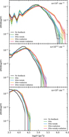 |
Fig. A.1 Volume distributions for cloud complexes with n > 10 cm−3 (top), big clouds with n > 101.5 cm−3 (middle), and clouds with n > 102 cm−3 (bottom). The lines show the median values, while the shaded regions show the 16th–84th percentile range. |
However, the distributions of cloud average densities (Fig. A.2) behave somewhat differently than the masses or volumes, in that the model with no feedback produces objects with the highest average densities at all scales, while prompt feedback only makes a small difference for cloud complexes.
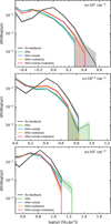 |
Fig. A.2 Same as Fig. A.1 but for the mean density distributions. Note that the limits on the horizontal axis are different in the panels. |
All Figures
|
Fig. 1 Cluster initial mass function, normalized to the total number of clusters (defined as stellar groups with ages <25 Myr) found in each simulation after 300 Myr. The error bars indicate the 16th and 84th percentiles computed using bootstrapping. The dashed line shows the slope of scale-free formation models, often associated with the initial cluster mass function (from A24, where more details are provided). |
| In the text | |
|
Fig. 2 Root node contours in projected gas density plots for different simulations (SNe in the top row, SNe+ radiation in the bottom row) and density thresholds (n > 10 cm−3 in the left column, and n > 102 cm−3 in the right column). As expected, astrodendro selects fewer and smaller structures with a higher density cutoff. |
| In the text | |
|
Fig. 3 Mass distributions for cloud complexes with n > 10 cm−3 (top), big clouds with n > 101.5 cm−3 (middle), and clouds with n > 102 cm−3 (bottom). The lines show the median values, while the shaded regions show the 16th–84th percentile range. All distributions shown contain structures from multiple snapshots, where consecutive snapshots are 25 Myr apart. The dashed line shows dN/d log(M) ∝ M−1, i.e., dN/dM ∝ M−2. |
| In the text | |
|
Fig. 4 Cloud mass distributions in 175 Myr time bins. Feedback is color-coded as in Fig. 3, and the number of clouds in each distribution is given in the legend. The lines show the median values, while the shaded regions show the 16th–84th percentile range. |
| In the text | |
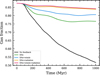 |
Fig. 5 Gas fraction, fgas (Eq. (2)), throughout time for all simulations (see the legend). |
| In the text | |
|
Fig. 6 Temperature as a function of density, color-coded by mass, for all gas in each simulation at time 750 Myr. |
| In the text | |
|
Fig. 7 Distribution of velocity dispersion against mass for cloud complexes (left), big clouds (center), and clouds (right). The median of the distribution is marked with a cross, while the 68th and 95th percentiles are shown as dashed and solid lines, respectively. Different models are color-coded as indicated in the legend. |
| In the text | |
|
Fig. A.1 Volume distributions for cloud complexes with n > 10 cm−3 (top), big clouds with n > 101.5 cm−3 (middle), and clouds with n > 102 cm−3 (bottom). The lines show the median values, while the shaded regions show the 16th–84th percentile range. |
| In the text | |
|
Fig. A.2 Same as Fig. A.1 but for the mean density distributions. Note that the limits on the horizontal axis are different in the panels. |
| In the text | |
Current usage metrics show cumulative count of Article Views (full-text article views including HTML views, PDF and ePub downloads, according to the available data) and Abstracts Views on Vision4Press platform.
Data correspond to usage on the plateform after 2015. The current usage metrics is available 48-96 hours after online publication and is updated daily on week days.
Initial download of the metrics may take a while.