| Issue |
A&A
Volume 705, January 2026
|
|
|---|---|---|
| Article Number | A3 | |
| Number of page(s) | 9 | |
| Section | Cosmology (including clusters of galaxies) | |
| DOI | https://doi.org/10.1051/0004-6361/202556116 | |
| Published online | 19 December 2025 | |
Quantifying the impact of detection bias from blended galaxies on cosmic shear surveys
1
Ruhr University Bochum, Faculty of Physics and Astronomy, Astronomical Institute (AIRUB), German Centre for Cosmological Lensing, 44780 Bochum, Germany
2
Argelander-Institut f. Astronomie, University of Bonn, Auf dem Hügel 71, 53121 Bonn, Germany
3
University of Innsbruck, Institute for Astro- and Particle Physics, Technikerstraße 25, 6020 Innsbruck, Austria
★ Corresponding author: This email address is being protected from spambots. You need JavaScript enabled to view it.
Received:
26
June
2025
Accepted:
20
October
2025
Abstract
Increasingly large areas in cosmic shear surveys lead to a reduction in statistical errors, necessitating increasingly accurate control of systematic errors. Previous studies have investigated one of these systematic effects: image overlap with bright foreground galaxies may cause some distant source galaxies to remain undetected. Since this overlap is more likely to occur in regions of high foreground density – which tend to be the regions in which the shear is largest – this detection bias would cause an underestimation of the shear correlation function. This detection bias adds to the possible systematic of image blending, in which nearby pairs or multiplets of images render shear estimates more uncertain, and thus may cause a reduction in their statistical weight. Based on simulations with data from the Kilo-Degree Survey, we investigated the conditions under which images are not detected. We find an approximate analytic expression for the detection probability in terms of the separation and brightness ratio relative to the neighbouring galaxies. Applying this fitting formula to weak-lensing ray tracing through the galaxy distribution in the Millennium Simulation, we estimate that the detection bias alone causes an underestimation of S8 = σ8√(Ωm/0.3) by almost 2%, and therefore cannot be neglected in current and forthcoming cosmic shear surveys.
Key words: gravitational lensing: weak / large-scale structure of Universe
© The Authors 2025
 Open Access article, published by EDP Sciences, under the terms of the Creative Commons Attribution License (https://creativecommons.org/licenses/by/4.0), which permits unrestricted use, distribution, and reproduction in any medium, provided the original work is properly cited.
This article is published in open access under the Subscribe to Open model. This email address is being protected from spambots. You need JavaScript enabled to view it. to support open access publication.
1. Introduction
Gravitational lensing refers to the distortion of light from distant galaxies as it passes through the gravitational potential of intervening matter along the line of sight. This distortion occurs because mass curves space-time, causing light to travel along curved paths. This effect is independent of the nature of the matter generating the gravitational field and thus probes the sum of dark and visible matter. When distortions in galaxy shapes are small, a statistical analysis including many background galaxies is required; this regime is known as weak gravitational lensing. One of the main observational probes in this regime is cosmic shear, which measures coherent distortions, or shears, in the observed shapes of distant galaxies induced by the large-scale structure of the Universe. By analysing correlations in the shapes of these background galaxies, we can infer statistical properties of the matter distribution and constrain cosmological parameters.
Although the large areas covered by recent imaging surveys, such as the Kilo-Degree Survey (KiDS; de Jong et al. 2013), significantly reduce statistical uncertainties in gravitational lensing studies, systematic effects must be examined in more detail. One such systematic is the effect of galaxy blending, which generally introduces two key challenges: first, some galaxies may not be detected at all; second, the shapes of blended galaxies may be measured inaccurately, leading to biased shear estimates. Although most recent studies focus on the latter effect (Hoekstra et al. 2017; Mandelbaum et al. 2018; Samuroff et al. 2018; Euclid Collaboration: Martinet et al. 2019; MacCrann et al. 2022; Nourbakhsh et al. 2022; Li et al. 2023; Zhang et al. 2025), the impact of undetected sources, first explored by Hartlap et al. (2011), has received limited attention since then. Hartlap et al. (2011) investigated this detection bias by selectively removing pairs of galaxies according to their angular separation and comparing the resulting shear correlation functions with and without such selection. Their findings showed that detection bias becomes particularly significant on angular scales below a few arcminutes, introducing errors of several percent. Given the magnitude of this effect, the detection bias cannot be ignored; this serves as the primary motivation for our study. Approaches such as Metadetection (Sheldon et al. 2020) incorporate object detection into the Metacalibration process and can mitigate shear biases from unrecognised blends at the same redshift; however, they do not address the more common and challenging case of cross-redshift blending. Such blends, in which galaxies at different redshifts are blended but not recognised as separate, can bias photometric redshifts and sample selection in ways that go beyond shear calibration, as discussed in Nourbakhsh et al. (2022).
Simply removing galaxies from the analysis (Hartlap et al. 2011) leads to object selection that depends on number density and thus also biases the cosmological inference, for instance by altering the redshift distribution of the analysed galaxies. While Hartlap et al. (2011) explored this effect using binary exclusion criteria based on angular separation, our work expands on this by modelling the detection probability as a continuous function of observable galaxy properties, specifically the flux ratio and projected separation relative to neighbouring sources. This approach enables a more nuanced and physically motivated treatment of blending. Based on this analysis, we aim to construct a detection probability function that assigns statistical weights to galaxies, rather than discarding them entirely, thereby mitigating bias without altering the underlying redshift distribution.
This paper is structured as follows. In Sect. 2, we describe the theoretical framework underlying our study. Section 3 presents the data used in our analysis. The methodology used to determine the detection probability function, along with the corresponding results, is presented in Sect. 4. We discuss our findings and conclude in Sect. 5.
2. Theoretical framework
The theoretical framework of this study is based on weak gravitational lensing (Bartelmann & Schneider 2001). The shape distortions of background galaxies are quantified using the shear, γ, and the convergence, κ, which are combined in the Jacobian matrix of the lens equation,
 (1)
(1)
where the complex shear is introduced with its two components, γ = γ1 + iγ2 = |γ| e2iϕ, with ϕ being the phase describing the direction of distortion. Assuming initially circular sources, the elongation of their images is described by the shear, which causes them to appear elliptical, whereas convergence quantifies the change in size. As neither convergence nor shear is observable on its own, the Jacobian matrix can be rewritten as
 (2)
(2)
where we introduce the reduced shear, g,
 (3)
(3)
which is a measurable quantity used in weak gravitational lensing. The observed image ellipticity provides an unbiased estimator of the reduced shear (Schramm & Kayser 1995; Seitz & Schneider 1997).
Because most distortions are weak and thus difficult to quantify, multiple statistical tools have been developed. A prominent example is the two-point shear correlation functions (2PSCFs), which measure how the shears at the positions of the source galaxies are correlated. The shear is decomposed into two components relative to the direction, ϕ, of the separation vector of each galaxy pair: the tangential and cross components, defined as
 (4)
(4)
The 2PSCFs are then defined as
 (5)
(5)
where θ denotes the projected separation between two galaxies.
The correlation functions are measured as follows. For a given galaxy field, all galaxy pairs with an angular separation θ are considered. The average of the product of tangential ellipticities, ⟨ϵt, iϵt, j⟩, of the pairs is then calculated as an estimator of ⟨γtγt⟩, assuming that the intrinsic ellipticities are uncorrelated. After applying the same procedure for the cross component, the shear correlation functions defined above can be calculated. The advantage of this method is that it is unaffected by bad pixels or masked regions because the mean shear vanishes.
It is expected that ξ× vanishes due to parity invariance in the Universe and is thus useful for checking certain systematics, whereas the other correlation functions, ξ±, are related to the power spectrum, Pκ(ℓ), as
 (6)
(6)
where J0 and J4 denote the zeroth and fourth-order Bessel functions of the first kind, respectively, while Pκ(ℓ) is the convergence power spectrum. Correlation functions from a data field are typically estimated by binning, with estimator given by Schneider et al. (2002)
 (7)
(7)
where ωi, j denotes the weights assigned to the galaxies and Δij(θ) = 1 if the separation between galaxies i and j falls within the bin centred on θ, and 0 otherwise.
3. Datasets
As mentioned in the previous sections, this work aims to quantify the detection bias resulting from blended galaxies in cosmic shear surveys. To this end, we simulated galaxies with GALSIM1 and inserted them into r-band detection images from the fourth data release of the Kilo-Degree Survey (KiDS). Following source extraction with SExtractor (v2.23.2; Bertin & Arnouts 1996), the resulting catalogue was compared with the simulated source list, allowing us to assess which galaxies are missed under specific conditions. Here, ‘detection’ refers to whether a simulated source is identified by SExtractor, and the detection probability is defined as the ratio of detected sources to inserted sources.
In the second part of this study, we used these detection probabilities as weights in the computation of shear correlation functions. The shear data were derived from the Millennium Simulation, complemented by galaxy properties from the catalogue of Henriques et al. (2015). This combined analysis allowed us to assess the impact of detection bias on cosmic shear measurements.
3.1. Kilo-Degree Survey data
The Kilo-Degree Survey is an optical imaging project that covers ∼7% of the extragalactic sky (∼1350 deg2). Observations are performed with the OmegaCAM wide-field camera2 on the VLT Survey Telescope (VST). The VST has a diameter of 2.6 m and is located at La Silla Paranal Observatory in Chile, operated by the European Southern Observatory (ESO; de Jong et al. 2013).
In this study, we used data from the fourth data release, KiDS-1000, which consists of 1006 survey tiles covering over 1000 deg2. Source detection, photometry, and general information about the data products of KiDS-1000 can be found in Kuijken et al. (2019), while the reduction of the KiDS data is explained in de Jong et al. (2015). Specifically, we used the r-band detection images, which are 1800 s exposures with a point spread function (PSF) full width at half maximum (FWHM)  and a mean airmass of 1.3.
Galaxies with reliable redshift and shape estimates are compiled into the publicly available KiDS-1000 SOM-gold catalogue, which contains 21 262 011 sources. This catalogue provides fluxes, magnitudes, half-light radii, redshifts, and ellipticities, which form the basis for our galaxy image simulations described in Sect. 4.
The photometric processing is described in Kuijken et al. (2019), and the redshift calibration – based on self-organising maps (SOMs) trained on spectroscopic samples – is detailed in Hildebrandt et al. (2021) and Wright et al. (2020).
Galaxy clusters in KiDS are identified using the Adaptive Matched Identifier of Clustered Objects (AMICO) algorithm (Bellagamba et al. 2018), which models the observed galaxy distribution as a superposition of cluster signal and background noise. After identifying the most significant cluster, AMICO subtracts its signal to search for additional candidates. The detection is performed on galaxies with r < 24, resulting in a catalogue of 7988 clusters in the redshift range 0.1 < z < 0.8 with signal to noise (S/N) > 3.5. We used the AMICO-DR3 catalogue, which includes only clusters from KiDS Data Release 3. Consequently, our analysis of cluster environments is limited to ∼450 deg2. More details on the AMICO-DR3 catalogue are available in Maturi et al. (2019).
3.2. Gravitational lensing simulations
As this study investigates the impact of blended galaxies, particularly the conditions under which they are detected or missed, cosmological simulations play a central role. They provide a controlled environment to systematically explore how detection is influenced by factors such as galaxy density, brightness, and proximity to neighbouring sources.
To simulate the mass distribution of the Universe, we used the Millennium Simulation (Springel et al. 2005), which is a DM-only N-body simulation with N = 21603 particles, each having a mass of mp = 8.6 × 10⁸ h−1 M⊙, in a cube with a comoving side length L = 500 h−1 Mpc. The growth of structure is tracked with these discrete dark matter particles from redshift z = 127 to z = 0 within the framework of Lambda Cold Dark Matter (ΛCDM) cosmology with parameters Ωm = 0.25, Ωb = 0.045, ΩΛ = 0.75, h = 0.73, ns = 1, and σ8 = 0.9. The simulation accurately traces the large-scale structure and the growth of dark matter halos, providing a robust framework for connecting cosmology to observational lensing data.
To connect the results of N-body simulations to the lensing observables, such as shear and convergence, we used the ray-tracing results presented in Hilbert et al. (2009). These results are based on the construction of a backward light cone along multiple lens planes from 37 snapshots at redshifts between z = 0 and z = 3.06, each with a FOV of 4° ×4° corresponding to a 40962 pixel grid.
As galaxies are the primary observables in weak lensing surveys, connecting dark matter simulations to real data requires a model of galaxy formation. To this end, we employed the semi-analytic galaxy catalogue of Henriques et al. (2015), which builds on the halo merger trees of the Millennium Simulation. This model incorporates baryonic processes such as gas cooling, star formation, and feedback, with parameters tuned to match observational constraints, primarily from early Sloan Digital Sky Survey (SDSS) data (Stoughton et al. 2002). The result is a realistic galaxy population useful for studying how detection biases propagate into weak lensing measurements.
4. Methods and results
To quantify the effects of blended galaxies, we investigated the detection probability of galaxies as a function of different parameters. For this purpose, we simulated galaxies with GALSIM, inserted them into the KiDS-1000 r-band detection images, and examined which sources were detected. In this section, we present two main methods for this purpose and their results. The first method investigated the detection probability of galaxies in galaxy cluster regions as a function of the clusters’ redshift and richness (Sect. 4.1), while the second method examined how the detection probability depends on various properties of the inserted sources or their neighbours (Sect. 4.2). The following procedure was applied to both methods:
-
For a field having N galaxies, we inserted N/10 simulated galaxies, which are simulated with GALSIM as described below.
-
A light profile with a Sérsic index n, randomly drawn from the distribution shown in Fig. 1, total flux F, and half-light radius re (Sérsic 1963) was created with GALSIM, with surface brightness profile
![Mathematical equation: $$ \begin{aligned} I(r) = \frac{F}{a_n\,r_{\mathrm{e} }^2}\, \exp [-b_n\,(r/r_\mathrm{e} )^{1/n}], \end{aligned} $$](/articles/aa/full_html/2026/01/aa56116-25/aa56116-25-eq10.gif) (8)
(8)where an determines flux normalisation and bn is a known coefficient calculated numerically by GALSIM based on the approximation of Ciotti & Bertin (1999). The generated light profile was convolved with the Moffat profile (Moffat 1969), an analytic model for the stellar PSF,
![Mathematical equation: $$ \begin{aligned} I(r) = \frac{\beta -1}{\pi r_0^2}[1+(r/r_0)^2]^{-\beta }, \end{aligned} $$](/articles/aa/full_html/2026/01/aa56116-25/aa56116-25-eq11.gif) (9)
(9)where β is set to
 , a typical value for a seeing-limited PSF, and r0 is the FWHM. We simulated galaxies by randomly selecting entries from the KiDS-1000 weak lensing SOM-gold catalogue, using their fluxes, half-light radii, and ellipticities as input parameters. The ellipticity was incorporated during the profile generation. After convolution with the PSF, each profile was binned according to the KiDS pixel scale of
  .
.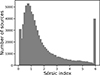
Fig. 1. Sérsic index distribution of galaxies in the COSMOS catalogue from Hernández-Martín et al. (2020), based on Sérsic profile fits provided by GALSIM (Mandelbaum et al. 2012; Rowe et al. 2015). The sharp peak in the final bin results from a Sérsic index limit in GALSIM, where all galaxies with an estimated index greater than 6.2 are grouped. When sampling Sérsic indices for our simulations, we drew from this distribution excluding the final bin. For details on the COSMOS catalogue, see Laigle et al. (2016).
-
These galaxies were randomly inserted into unmasked regions of the corresponding r-band detection image, where the two mask images of KiDS-1000, one for the north and the other for the south, were used to determine the masked regions.
-
SExtractor (v2.23.1) was run on the source-injected images, producing 1006 catalogues corresponding to the number of detection images.
-
These catalogues were compared with the injected galaxy list to assess the retrieval rate, yielding the detection probability for each image field. We associated each injected input galaxy with SExtractor detections using a nearest-neighbour match within a radius of 3.6 pixels3. For matching, we used spatial.KDTree from scipy4, which is a nearest-neighbour finding algorithm developed by Maneewongvatana & Mount (1999). In cases where multiple input galaxies overlapped but only one detection was identified by SExtractor, the input galaxy closest to the detection centroid was counted as detected, while the others were considered undetected. This ensures that each detection is uniquely linked to at most one input source.
4.1. Method 1: Cluster regions
Through the complex interplay of dark and baryonic matter across cosmic time, galaxies formed and aggregated via gravitational interactions, eventually giving rise to galaxy clusters. These clusters are now prominent overdense regions in the Universe, characterised by a high galaxy number density. Consequently, blending effects are expected to be particularly pronounced in cluster environments, where the shear is large. The primary goal of this method is to explore how the detection probability of galaxies varies as a function of cluster richness and redshift.
After injecting simulated sources into the images, we assigned each source to its nearest cluster, as identified in the AMICO-DR3 catalogue. A source is excluded from the analysis if its physical separation from the assigned cluster exceeds the cluster’s virial radius R2005.
We investigated the detection probability of sources in cluster regions as a function of cluster richness and redshift. We used the ‘intrinsic richness’6 of galaxy clusters in the AMICO-DR3 catalogue (Maturi et al. 2019), which is defined as the sum of the probabilities that galaxies belong to the j-th cluster,
 (10)
(10)
where m* is the characteristic magnitude in the Schechter luminosity function (Schechter 1976), which varies with redshift. We restricted our analysis to clusters with intrinsic richness λ ≥ 5 to minimise contamination by sparse groups or spurious detections.
Figure 2 shows the probability of detection of injected sources within clusters, defined as the recovery rate of galaxies injected in each cluster region. The dotted line indicates the average detection probability as a function of the cluster richness, and the dashed line shows it as a function of the cluster redshift. The detection probability tends to decrease with increasing richness and increase with redshift. The latter trend may reflect the reduced brightness of the contaminating cluster members at higher redshifts, making injected sources easier to detect.
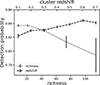 |
Fig. 2. Detection probability as a function of richness (bottom axis) and redshift (top axis) for the AMICO-DR3 galaxy clusters, shown with dotted and dashed lines, respectively. As the catalogue contains very few clusters with high richness (greater than 70), clusters are divided into five logarithmically spaced richness bins and seven linearly spaced redshift bins. The error bars represent the standard errors of the detection probability. |
Our method follows a similar approach to that of Kleinebreil et al. (2025), who injected synthetic galaxies into KiDS tiles using GALSIM to assess detection bias in dense environments. While their analysis uses the first eROSITA All-Sky Survey (eRASS1) cluster sample, we used a different cluster catalogue and adopted a simplified framework. Although both catalogues contain a comparable number of clusters, the eRASS1 sample covers a significantly larger area on the sky (∼1000 deg2 vs ∼450 deg2 in our case), allowing for better statistical robustness and spatial sampling. They observed that detection bias strength increases with both cluster redshift and richness, contrasting with our findings of a mild increase in detection probability with cluster redshift. However, a direct comparison is not straightforward due to methodological and data-related differences. Their larger sky coverage permits measurement of detection probability as a function of distance from the cluster centre. Moreover, their redshift trend is derived from tomographic and radial bins, while we average over full cluster fields. These differences in scale and technique likely contribute to the divergent trends observed.
Our aim was to model the detection probability as a function of both the cluster richness and the redshift. However, this could not be robustly achieved due to the limited number of clusters in the current catalogue and the strong correlation between these two parameters. Additionally, some clusters span large areas on the sky, so injected sources may blend with unrelated field galaxies rather than cluster members. Although this issue could be mitigated with colour-based membership information, such data are not available in AMICO-DR3. Despite these limitations, the richness–redshift approach remains promising for future studies. With more comprehensive catalogues and richer cluster data, a more accurate model could be developed. In the present work, we complemented this method with a second approach based on the local properties of the inserted sources and their immediate neighbours, which we describe in the next section.
4.2. Method 2: Source and neighbour properties
In the second method, we investigate the detection probability of injected sources as a function of their intrinsic properties and those of their nearest-neighbouring galaxies, which may be either another injected source or an existing KiDS galaxy in the same tile. In rare cases, an undetected KiDS galaxy may lie closer to an injected source than the identified nearest neighbour. As these galaxies do not appear in the detection catalogue, they cannot be explicitly matched; however, we expect their statistical impact to be negligible for the overall detection probability analysis.
The intrinsic properties of injected galaxies are known by construction, as they are simulated using KiDS-1000 SOM-Gold catalogue entries. For neighbouring galaxies that are already present in the KiDS r-band detection images, the corresponding properties are available in the source catalogue of each KiDS tile. We used the input properties for injected galaxies, since their measured quantities in the blended images would be affected by nearby sources. For KiDS galaxies, by contrast, we used their measured catalogue properties, as these are derived from the original images without injections. This approach allowed us to quantify blending effects in a more general and flexible framework that does not rely on the presence of galaxy clusters.
To capture trends across a range of brightness levels, we analysed each parameter in six linearly spaced magnitude bins of the injected sources: four bins covering the r-band magnitude range 20–22 and two bins covering 22–24. Nearest neighbours were restricted to galaxies. To exclude stars and unreliable detections from the neighbour sample, we used the SG2DPHOT7 flag provided in the KiDS multi-band catalogue and retained only neighbours with a value of 0.
Figure 3 shows the detection probability as a function of several source and neighbour parameters. In these plots, subscripts ‘s’ and ‘n’ refer to the properties of the inserted source and its nearest neighbour, respectively.
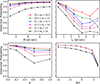 |
Fig. 3. Detection probability of injected source galaxies as a function of four environmental parameters: angular separation to the nearest neighbour (upper left), half-light radius of the nearest neighbour (upper right), proximity parameter (lower left; see Sect. 4.2), and magnitude difference between the injected source and its neighbour (lower right). Curves correspond to different magnitude bins of the injected sources, as indicated in the legend. |
-
Separation: The first property investigated was the projected separation between the source and its nearest neighbour. As shown in the upper left panel of Fig. 3, the detection probability generally increases with separation, as expected. However, the dependence is relatively weak, with values ranging between approximately 0.75 and 1.0, and the behaviour varies across flux bins.
-
Half-light radius of the nearest neighbour: The next parameter examined was the half-light radius of the nearest neighbour, shown in the upper-right panel of Fig. 3. In all flux bins, the detection probability decreases with increasing half-light radius, as expected. This dependence is more pronounced than that on separation: detection probabilities can drop below 40% for sources located near large neighbours. As with the separation, the detailed behaviour varies among flux bins.
-
Proximity parameter: To account for both angular size and separation, we define the ‘proximity parameter’ as
 (11)
(11)where re, s and re, n are the half-light radii of the source and the neighbour, respectively, and θ is their projected separation. This parameter reflects how close two objects appear relative to their combined sizes. The lower-left panel of Fig. 3 shows the detection probability as a function of this parameter. As in the case of separation alone, the dependence is moderate. This suggests that while size and separation both influence detectability, their combined effect through the proximity parameter is still weaker than the influence of neighbour size alone. Moreover, a single functional form cannot capture the behaviour across all flux bins.
-
Magnitude difference: In the lower-right panel of Fig. 3, we present the detection probability as a function of the magnitude difference between the injected source and its nearest neighbour, defined as Δm = ms − mn. Apart from the faintest flux bin, the behaviour is consistent across all bins, following a smooth and well-defined trend. The faintest magnitude bin exhibits a lower detection probability even at very negative Δm (i.e. effectively isolated), reflecting the baseline single-object completeness at that magnitude. While normalising the curves at Δm = −4 would collapse them to a common shape, we retained the unnormalised form to show that faint sources are intrinsically harder to detect, independent of blending. Owing to this robustness and simplicity, the magnitude difference was selected as the primary parameter for subsequent modelling and analysis.
We examined the detection probability as a function of Δm in four different separation bins, as shown in Fig. 4. We adopted a fitting function for the behaviour of the detection probability as a function of the two driving properties: the magnitude difference and the separation. To accomplish this, we adopted a model function whose choice is motivated by its ability to provide a good fit to the measurements, while still being relatively simple,
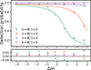 |
Fig. 4. Upper panel: Detection probability as a function of magnitude difference in four separation bins between 0 and 5 arcseconds, with the fit function (12) plotted for each bin. The detection probability behaviour in higher separation bins coincides with the purple line and is therefore omitted for clarity. Residuals between the model fit and the data points for each separation bin are shown. |
 (12)
(12)
where Δm is the magnitude difference and θ is the angular separation. The parameters b and δ are free parameters and are determined via non-linear least-squares fitting using the curve_fit function from the scipy package8. The best-fitting values found are b = (1.30 ± 0.03) arcsec−1 and δ = 0.50 ± 0.04.
Overall, the model captures the data trends well: residuals are below 5% for the majority of points and under 10% for all, except in the largest Δm bin in the separation range 4 < θ[″]< 5. We used this model function in our subsequent cosmological analysis, where we aim to quantify how undetected sources resulting from blending can affect cosmic shear measurements.
4.3. Cosmological analysis
To quantify the impact of undetected sources due to blending on cosmic shear measurements, we incorporated the constrained detection probability function to assign weights to galaxies. We used these weights as inputs in the computation of the 2PSCFs, enabling a direct comparison of cosmic shear signals with and without accounting for blending effects. Section 4.3.1 details the weight assignment procedure, while the shear correlation function measurements are presented in Sect. 4.3.2.
4.3.1. Assigning weights
For this analysis, we used the Henriques et al. (2015) galaxy catalogue, employing the galaxy positions, redshifts, and r-band magnitudes. The magnitudes were corrected for both magnification and galactic dust extinction. We selected galaxies on the basis of two criteria:
-
Redshift: Galaxies were selected in five tomographic redshift bins, which corresponded to those used in the KiDS-1000 cosmic shear analysis (Asgari et al. 2021), listed in the second column of Table 1. In regions where a galaxy’s redshift overlaps multiple bins, random assignment ensures that the overall distribution in each bin remains consistent with KiDS.
Table 1.Data properties per tomographic redshift bin.
-
Flux: Within each redshift bin, galaxies were further selected to match the flux distribution observed in KiDS-1000.
For each galaxy, we computed its detection probability using the model constructed in Sect. 4.2, based on its projected separation from the nearest neighbour and the magnitude difference between the two,
 (13)
(13)
where ω denotes the detection probability, while θ and Δm are the separation and magnitude difference, respectively. This detection probability was then assigned as a weight to the galaxy and used in the subsequent shear correlation analysis. To locate the nearest neighbours and calculate the separations between galaxies and their neighbours, we again used the spatial.KDTree from scipy.
Although the detection probability weighting alters the effective contribution of galaxies at different redshifts (see Fig. 5), this effect is a consequence of the underlying detection bias being modelled. Unlike binary selection schemes, such as those applied by Hartlap et al. (2011), our method retains all galaxies and reflects their physical likelihood of being detected. The change in the redshift distribution is therefore not imposed by artificial cuts but emerges naturally from the blending conditions in the data.
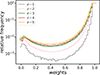 |
Fig. 5. Distribution of the calculated detection probabilities (i.e. assigned weights) of galaxies in each z-bin. A primary peak is visible near unity, while a secondary peak appears near zero, particularly in the lower redshift bins. |
4.3.2. Calculating 2PSCFs
The ray-tracing results from the Millennium Simulation provide the components of the Jacobian matrix on 64 redshift slices, each represented by a 4096 × 4096 pixel grid. From these data, we computed key lensing quantities: convergence, which traces the matter distribution, and the reduced shear, which serves as the input for computing the shear correlation functions.
Since the galaxy positions in the Henriques et al. (2015) catalogue are derived from dark matter halo coordinates, they are expressed in angular units (radians) rather than pixel coordinates. To associate lensing quantities with galaxies, we projected the galaxy positions onto the pixel grid and assigned them the reduced shear values of the nearest grid points.
A summary of the data used in the shear correlation function calculations is provided in Table 1. The average number of galaxies per field and their corresponding mean weights are listed in the third and fourth columns. We observe that the average weight tends to decrease with redshift, reflecting the increasing difficulty of detecting high-redshift galaxies, which are fainter and more likely to be blended with brighter neighbours.
Figure 5 shows the distribution of detection probabilities (assigned weights) across redshift bins. While most galaxies have weights close to unity, a secondary peak near zero is also visible, especially in lower redshift bins. This feature is attributed to the larger isophotal sizes of low-redshift galaxies, which increase the likelihood of blending with nearby sources.
We performed the 2PSCFs calculations using TreeCorr (Jarvis et al. 2004) in eight logarithmically spaced angular separation bins between  and 120′, consistent with the binning strategy of the KiDS-1000 cosmic shear analysis. This approach optimised the balance between S/N and statistical robustness: too few bins can obscure scale-dependent effects, while too many would introduce noise and reduce statistical significance. Initially, the correlation functions were computed without applying any weights. The analysis was then repeated, incorporating galaxy detection probabilities as multiplicative weights.
Figure 6 presents the bias in the 2PSCFs due to blending, defined analogously to Hartlap et al. (2011) as
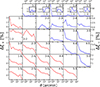 |
Fig. 6. Bias (Eq. (14)) in the 2PSCFs. The red colour indicates the bias in ξ+, while the blue colour indicates the bias in ξ−. Each plot is labelled with the corresponding tomographic redshift bin pair. |
 (14)
(14)
where nw denotes the non-weighted correlation functions and w denotes the weighted correlation functions. The relative bias is considerably smaller in ξ+ than in ξ− and decreases with increasing angular separation, indicating that the blending-induced bias predominantly affects small physical scales. This is consistent with theoretical expectations: the Bessel function J4 in Eq. (6), which defines the filtering of the power spectrum for ξ−, peaks at ℓθ ≈ 5, making ξ− more sensitive to smaller scales. Conversely, ξ+ is dominated by large-scale modes as J0 peaks at ℓθ = 0. The large bias in ξ− at the lowest redshift bin stems from the extremely small amplitude of the correlation function itself in this regime.
We compared our results with those of Hartlap et al. (2011), who quantified the impact of density-dependent galaxy selection on two-point shear correlations. They reported two fractional biases: one that included both the effect of density-dependent selection and changes in the redshift distribution, and another that included only the density-dependent selection effect (with the redshift distribution corrected). Our results are consistent with the latter: the amplitude of the bias is a few percent, increases towards smaller scales, and is stronger for ξ− than for ξ+. This agreement indicates that our model captures the density-dependent selection effects accurately, while the effects of the change in the redshift distribution of galaxies are not captured. Unlike Hartlap et al. (2011), we probed different redshift bin combinations, revealing that for ξ− the bias can reach ∼50% at the smallest scales for the lowest-redshift cross-correlations (1-1, 1-2, 1-3, 1-4, 1-5), while for other combinations it remains below 5%. For ξ+, the bias remains small (-1–2%) and decreases from smaller to larger separations, becoming slightly negative at the largest scales.
4.3.3. Cosmological parameters
To assess the impact of this detection bias on cosmological inference, we performed an analysis based on the likelihood
![Mathematical equation: $$ \begin{aligned} \mathfrak{L} \propto \mathrm{exp} \left( -0.5[\boldsymbol{\xi }-\boldsymbol{\xi }_\mathrm{m} ]^\mathrm{t}\mathrm{C} ^{-1}[\boldsymbol{\xi }-\boldsymbol{\xi }_\mathrm{m} ]\right), \end{aligned} $$](/articles/aa/full_html/2026/01/aa56116-25/aa56116-25-eq20.gif) (15)
(15)
where the data vector of observed correlation functions is given by ξ = [ξ+(θ1),…,ξ+(θ8),ξ−(θ1),…,ξ−(θ8)]t. These functions were measured using the Henriques et al. (2015) catalogue in the same eight angular separation bins between  and 120′. We computed the model prediction vector, ξm, from a theoretical shear power spectrum generated with pyccl (v3.0.1)9. The covariance matrix, C, was adopted from the KiDS-1000 cosmic shear analysis (Asgari et al. 2021).
Table 2 lists the cosmological parameters and priors used in the likelihood analysis. The baryonic matter density parameter, Ωb, was fixed, while the cold dark matter density, Ωc, and the amplitude of the power spectrum, σ8, were allowed to vary. The likelihood was first evaluated using unweighted correlation functions, followed by an evaluation that included the detection probability weights.
Cosmological parameters and their priors used in fiducial cosmology.
Table 3 summarises the posterior peaks and 1σ uncertainties of the three cosmological parameters inferred from the cosmic shear likelihood, for correlation functions evaluated with and without detection probability weights. The very small error bars obtained here should not be directly compared to those from real surveys, as they reflect an idealised setup excluding shape noise and shear-calibration uncertainties. This choice was deliberate to isolate and quantify the impact of blending on cosmological parameter estimation. Moreover, the recovered parameters lie close to the Planck Collaboration VI (2020) cosmology, as expected, since the Henriques et al. (2015) galaxy catalogue is constructed assuming that cosmology.
Recovered cosmological parameters from the cosmic shear likelihood with and without weights.
We find fractional biases of ∼2.35% in Ωc and ∼0.66% in σ8, resulting in an overall bias of ∼1.88% in the derived parameter  . The shift towards lower Ωm, σ8, and S8 when weights are applied is consistent with blending preferentially removing or down-weighting detections that would otherwise enhance the small-scale lensing signal. It is important to note that this estimate excludes parameter degeneracies and does not account for additional systematic effects such as baryonic feedback, intrinsic alignments, or shear-calibration biases.
5. Conclusions
This study investigates the impact of galaxy non-detections on cosmic shear measurements, an effect first examined by Hartlap et al. (2011) but rarely revisited since. This effect adds to that of blending sources, which render shear measurements less reliable and have been extensively studied (Hoekstra et al. 2017; Mandelbaum et al. 2018; Samuroff et al. 2018; Euclid Collaboration: Martinet et al. 2019). With the increasing demand for precise systematic control in Stage-IV cosmological surveys, we revisit and extend Hartlap et al. (2011), enhancing our understanding of galaxy detection probabilities under varying conditions. Specifically, rather than excluding galaxy pairs using an ad-hoc separation criterion, we empirically derive detection probabilities based on KiDS-1000 data.
We initially explored detection biases in the vicinity of galaxy clusters. The detection probability shows a mild increase with cluster redshift and a possible decrease with cluster richness, although these trends are not strongly significant and are accompanied by large uncertainties at higher richness, likely due to the limited number of clusters in the catalogue and the strong correlation between cluster parameters.
To address this, we pursued an alternative strategy by analysing the detection probability of inserted sources as a function of their intrinsic properties and those of their neighbouring galaxies, across different flux bins. We find that the detection probability exhibits a consistent dependence on the r-band magnitude difference between a source and its nearest neighbour, regardless of the source flux. Interestingly, this contrasts with the results of Samuroff et al. (2018), who report a weaker dependence on the magnitude difference relative to the angular separation. This discrepancy highlights the importance of first establishing galaxy detectability before assessing the precise impact of blending.
We constrained our detection probability function to depend both on the magnitude difference and the separation. In crowded galaxy fields, blending can arise not only from the closest neighbouring galaxy but also from multiple nearby sources simultaneously. Although the second-nearest or undetected neighbours can, in principle, influence the detection outcome, their contribution is statistically negligible for our analysis.
To quantify this bias in cosmic shear surveys, we employed our detection probability function to assign weights to galaxies, which we then used to compute shear correlation functions. A key advantage of this weighting scheme is that it preserves the full galaxy sample while down-weighting less reliably detected sources. As shown in Fig. 6, the bias is most prominent on small angular scales and in the ξ− correlation function. Our likelihood analysis shows that this bias can lead to a fractional shift of 1.88% in the S8 parameter, underscoring its relevance for precision weak-lensing studies.
It should be noted that this source non-detection effect provides a lower bound on the impact of blending on cosmic shear measurements. Detected yet blended galaxies are typically assigned lower weights owing to the increased uncertainty of their shear estimates.
In summary, we find that the flux ratio between a galaxy and its neighbours, along with their angular separation, are the key determinants of detectability. The detection probability function derived in this work provides a valuable tool for future mitigation of detection-related systematics – either through the development of new algorithms or by enhancing existing ones, such as Metadetection (Sheldon et al. 2020), to identify and correct blended sources more effectively.
GALSIM is an open-source image simulation tool for creating realistic astronomical images. Its key advantage lies in offering a wide range of options for transformations, rotations, convolutions, and other image-processing operations. For details, see Rowe et al. (2015).
OmegaCAM is a wide-field camera on the VST with a resolution of 268 Megapixels, a field-of-view (FOV) of 1° ×1° and a pixel scale of  /pix. For more information about OmegaCAM, see Kleijn et al. (2013).
We used a matching tolerance of 3.6 pixels ( at the KiDS pixel scale), which corresponds to the PSF FWHM of KiDS r-band detection images.
We used the ΛCDM model with parameters from Maturi et al. (2019) in both the calculation of the virial radii from AMICO catalogue masses and to determine physical distances from pixels.
The AMICO-DR3 catalogue provides both apparent and intrinsic richness. Since the intrinsic richness aligns more closely with conventional definitions of galaxy clusters, we adopted it exclusively.
SG2DPHOT: KiDS-CAT star-galaxy classification bitmap based on r-band source morphology. Values are: 1 = high-confidence star candidate, 2 = unreliable source, 4 = star based on star-galaxy separation criteria, 0 = other sources (e.g. galaxies). Neighbours with a flag value of 1 or 4 are excluded.
Acknowledgments
We would like to thank Sven Heydenreich and Laila Linke for useful discussions during the project. EG acknowledges the support from the Deutsche Forschungsgemeinschaft (DFG) SFB1491. TS acknowledges support from the Austrian Research Promotion Agency (FFG) and the Federal Ministry of the Republic of Austria for Innovation, Mobility, and Infrastructure (BMIMI) via grants 899537, 900565, and 911971. The data used in this work are based on observations made with ESO Telescopes at the La Silla Paranal Observatory under programme IDs 177.A-3016, 177.A-3017, 177.A-3018 and 179.A-2004, and on data products produced by the KiDS Consortium. The KiDS production team acknowledges support from the DFG, ERC, NOVA and NWO-M grants; Target; the University of Padova, and the University Federico II (Naples). This work was supported by a grant of the German Centre of Cosmological Lensing, hosted at Bochum University. The Millennium Simulation datasets were constructed as part of activities of the German Astrophysical Virtual Observatory.
References
- Asgari, M., Lin, C.-A., Joachimi, B., et al. 2021, A&A, 645, A104 [NASA ADS] [CrossRef] [EDP Sciences] [Google Scholar]
- Bartelmann, M., & Schneider, P. 2001, Phys. Rep., 340, 291 [Google Scholar]
- Bellagamba, F., Roncarelli, M., Maturi, M., & Moscardini, L. 2018, MNRAS, 473, 5221 [NASA ADS] [CrossRef] [Google Scholar]
- Bertin, E., & Arnouts, S. 1996, A&AS, 117, 393 [NASA ADS] [CrossRef] [EDP Sciences] [Google Scholar]
- Ciotti, L., & Bertin, G. 1999, A&A, 352, 447 [NASA ADS] [Google Scholar]
- de Jong, J. T. A., Kleijn, G. A. V., Kuijken, K., & Valentijn, E. A. 2013, Exp. Astron., 35, 25 [NASA ADS] [CrossRef] [Google Scholar]
- de Jong, J. T., Verdoes Kleijn, G. A., Boxhoorn, D. R., et al. 2015, A&A, 582, A62 [NASA ADS] [CrossRef] [EDP Sciences] [Google Scholar]
- Euclid Collaboration (Martinet, N., et al.) 2019, A&A, 627, A59 [NASA ADS] [CrossRef] [EDP Sciences] [Google Scholar]
- Hartlap, J., Hilbert, S., Schneider, P., & Hildebrandt, H. 2011, A&A, 528, A51 [NASA ADS] [CrossRef] [EDP Sciences] [Google Scholar]
- Henriques, B. M., White, S. D., Thomas, P. A., et al. 2015, MNRAS, 451, 2663 [CrossRef] [Google Scholar]
- Hernández-Martín, B., Schrabback, T., Hoekstra, H., et al. 2020, A&A, 640, A117 [EDP Sciences] [Google Scholar]
- Hilbert, S., Hartlap, J., White, S., & Schneider, P. 2009, A&A, 499, 31 [NASA ADS] [CrossRef] [EDP Sciences] [Google Scholar]
- Hildebrandt, H., van den Busch, J., Wright, A., et al. 2021, A&A, 647, A124 [NASA ADS] [CrossRef] [EDP Sciences] [Google Scholar]
- Hoekstra, H., Viola, M., & Herbonnet, R. 2017, MNRAS, 468, 3295 [NASA ADS] [CrossRef] [Google Scholar]
- Jarvis, M., Bernstein, G., & Jain, B. 2004, MNRAS, 352, 338 [Google Scholar]
- Kleijn, G. A. V., Kuijken, K. H., Valentijn, E. A., et al. 2013, Exp. Astron., 35, 103 [Google Scholar]
- Kleinebreil, F., Grandis, S., Schrabback, T., et al. 2025, A&A, 695, A216 [NASA ADS] [CrossRef] [EDP Sciences] [Google Scholar]
- Kuijken, K., Heymans, C., Dvornik, A., et al. 2019, A&A, 625, A2 [NASA ADS] [CrossRef] [EDP Sciences] [Google Scholar]
- Laigle, C., McCracken, H. J., Ilbert, O., et al. 2016, ApJS, 224, 24 [Google Scholar]
- Li, S.-S., Kuijken, K., Hoekstra, H., et al. 2023, A&A, 670, A100 [NASA ADS] [CrossRef] [EDP Sciences] [Google Scholar]
- MacCrann, N., Becker, M. R., McCullough, J., et al. 2022, MNRAS, 509, 3371 [Google Scholar]
- Mandelbaum, R., Hirata, C. M., Leauthaud, A., Massey, R. J., & Rhodes, J. 2012, MNRAS, 420, 1518 [NASA ADS] [CrossRef] [Google Scholar]
- Mandelbaum, R., Lanusse, F., Leauthaud, A., et al. 2018, MNRAS, 481, 3170 [NASA ADS] [CrossRef] [Google Scholar]
- Maneewongvatana, S., & Mount, D. M. 1999, arXiv e-prints [arXiv:cs/9901013] [Google Scholar]
- Maturi, M., Bellagamba, F., Radovich, M., et al. 2019, MNRAS, 485, 498 [Google Scholar]
- Moffat, A. 1969, A&A, 3, 455 [Google Scholar]
- Nourbakhsh, E., Tyson, J. A., Schmidt, S. J., et al. 2022, MNRAS, 514, 5905 [NASA ADS] [CrossRef] [Google Scholar]
- Planck Collaboration VI. 2020, A&A, 641, A6 [NASA ADS] [CrossRef] [EDP Sciences] [Google Scholar]
- Rowe, B. T., Jarvis, M., Mandelbaum, R., et al. 2015, Astron. Comput., 10, 121 [NASA ADS] [CrossRef] [Google Scholar]
- Samuroff, S., Bridle, S., Zuntz, J., et al. 2018, MNRAS, 475, 4524 [NASA ADS] [CrossRef] [Google Scholar]
- Schechter, P. 1976, ApJ, 203, 297 [Google Scholar]
- Schneider, P., van Waerbeke, L., Kilbinger, M., & Mellier, Y. 2002, A&A, 396, 1 [NASA ADS] [CrossRef] [EDP Sciences] [Google Scholar]
- Schramm, T., & Kayser, R. 1995, A&A, 299, 1 [NASA ADS] [Google Scholar]
- Seitz, C., & Schneider, P. 1997, A&A, 318, 687 [NASA ADS] [Google Scholar]
- Sérsic, J. 1963, Boletin de la Asociacion Argentina de Astronomia La Plata Argentina, 6, 41 [Google Scholar]
- Sheldon, E. S., Becker, M. R., MacCrann, N., & Jarvis, M. 2020, ApJ, 902, 138 [CrossRef] [Google Scholar]
- Springel, V., White, S. D., Jenkins, A., et al. 2005, Nature, 435, 629 [Google Scholar]
- Stoughton, C., Lupton, R. H., Bernardi, M., et al. 2002, AJ, 123, 485 [Google Scholar]
- Wright, A., Hildebrandt, H., Van den Busch, J. L., & Heymans, C. 2020, A&A, 637, A100 [NASA ADS] [CrossRef] [EDP Sciences] [Google Scholar]
- Zhang, S., Li, S.-S., & Hoekstra, H. 2025, A&A, 702, A166 [NASA ADS] [CrossRef] [EDP Sciences] [Google Scholar]
All Tables
Recovered cosmological parameters from the cosmic shear likelihood with and without weights.
All Figures
|
Fig. 1. Sérsic index distribution of galaxies in the COSMOS catalogue from Hernández-Martín et al. (2020), based on Sérsic profile fits provided by GALSIM (Mandelbaum et al. 2012; Rowe et al. 2015). The sharp peak in the final bin results from a Sérsic index limit in GALSIM, where all galaxies with an estimated index greater than 6.2 are grouped. When sampling Sérsic indices for our simulations, we drew from this distribution excluding the final bin. For details on the COSMOS catalogue, see Laigle et al. (2016). |
| In the text | |
|
Fig. 2. Detection probability as a function of richness (bottom axis) and redshift (top axis) for the AMICO-DR3 galaxy clusters, shown with dotted and dashed lines, respectively. As the catalogue contains very few clusters with high richness (greater than 70), clusters are divided into five logarithmically spaced richness bins and seven linearly spaced redshift bins. The error bars represent the standard errors of the detection probability. |
| In the text | |
|
Fig. 3. Detection probability of injected source galaxies as a function of four environmental parameters: angular separation to the nearest neighbour (upper left), half-light radius of the nearest neighbour (upper right), proximity parameter (lower left; see Sect. 4.2), and magnitude difference between the injected source and its neighbour (lower right). Curves correspond to different magnitude bins of the injected sources, as indicated in the legend. |
| In the text | |
|
Fig. 4. Upper panel: Detection probability as a function of magnitude difference in four separation bins between 0 and 5 arcseconds, with the fit function (12) plotted for each bin. The detection probability behaviour in higher separation bins coincides with the purple line and is therefore omitted for clarity. Residuals between the model fit and the data points for each separation bin are shown. |
| In the text | |
|
Fig. 5. Distribution of the calculated detection probabilities (i.e. assigned weights) of galaxies in each z-bin. A primary peak is visible near unity, while a secondary peak appears near zero, particularly in the lower redshift bins. |
| In the text | |
|
Fig. 6. Bias (Eq. (14)) in the 2PSCFs. The red colour indicates the bias in ξ+, while the blue colour indicates the bias in ξ−. Each plot is labelled with the corresponding tomographic redshift bin pair. |
| In the text | |
Current usage metrics show cumulative count of Article Views (full-text article views including HTML views, PDF and ePub downloads, according to the available data) and Abstracts Views on Vision4Press platform.
Data correspond to usage on the plateform after 2015. The current usage metrics is available 48-96 hours after online publication and is updated daily on week days.
Initial download of the metrics may take a while.