| Issue |
A&A
Volume 705, January 2026
|
|
|---|---|---|
| Article Number | A69 | |
| Number of page(s) | 8 | |
| Section | The Sun and the Heliosphere | |
| DOI | https://doi.org/10.1051/0004-6361/202556214 | |
| Published online | 06 January 2026 | |
Collisional and magnetic effects on the polarization of the solar oxygen infrared triplet
Astronomy and Space Science Department, Faculty of Science, King Abdulaziz University, PO Box 80203 Jeddah, 21589
Saudi Arabia
★ Corresponding authors: This email address is being protected from spambots. You need JavaScript enabled to view it.
; This email address is being protected from spambots. You need JavaScript enabled to view it.
Received:
1
July
2025
Accepted:
13
November
2025
Abstract
Context. The scattering polarization of the infrared (IR) triplet of neutral oxygen (O I) near 777 nm provides a powerful diagnostic of solar atmospheric conditions. However, interpreting such polarization requires a rigorous treatment of isotropic depolarizing collisions between O I atoms and neutral hydrogen.
Aims. We aim to investigate the combined effects of collisional and magnetic depolarization in shaping the alignment of O I levels (and thus the polarization of the O I IR triplet).
Methods. We compute, for the first time, a comprehensive set of collisional depolarization and polarization transfer rates for the relevant O I energy levels. These rates are incorporated into a multilevel atomic model, and the statistical equilibrium equations (SEE) are solved to quantify the impact of collisions and magnetic fields on atomic alignment.
Results. Our calculations indicate that elastic collisions with neutral hydrogen, together with the Hanle effect of turbulent magnetic fields stronger than about 20 G, efficiently suppress the bulk of the atomic alignment in deep photospheric conditions where hydrogen densities exceed nH ∼ 1016 cm−3. In the chromosphere, however, the lower hydrogen density weakens collisional depolarization, allowing polarization to persist.
Conclusions. Our results are consistent with a chromospheric origin for the linear polarization signals of the O I IR triplet. Future studies should combine accurate non-LTE radiative transfer with reliable collisional rates in order to achieve fully consistent modeling.
Key words: atomic processes / line: formation / Sun: chromosphere / Sun: magnetic fields / Sun: photosphere
© The Authors 2026
 Open Access article, published by EDP Sciences, under the terms of the Creative Commons Attribution License (https://creativecommons.org/licenses/by/4.0), which permits unrestricted use, distribution, and reproduction in any medium, provided the original work is properly cited.
This article is published in open access under the Subscribe to Open model. This email address is being protected from spambots. You need JavaScript enabled to view it. to support open access publication.
1. Introduction
In recent decades, there has been growing interest in finding reliable ways to detect, understand, and measure magnetic fields in the Sun’s photosphere and chromosphere. The advent of high-sensitivity polarimetry enabled the detection of subtle polarization signals in numerous spectral lines, particularly those of the so-called second solar spectrum (e.g., Stenflo 1994; Landi Degl’Innocenti & Landolfi 2004; Trujillo Bueno 2001). These weak polarization signatures, often shaped by the Hanle effect, provide valuable insights into the geometry and strength of magnetic fields in regions where the Zeeman effect alone is insufficient. However, interpreting scattering polarization signals observed in spectral lines in terms of solar magnetic fields remains notoriously challenging due to the complex interplay among atomic polarization, radiative transfer, magnetic fields, and collisional depolarization processes.
Since the 1990s, numerous studies have investigated various spectral lines and mechanisms for diagnosing solar magnetism. In this context, some attention has been given to the O I infrared (IR) triplet–a promising diagnostic target that would benefit from a more rigorous treatment, especially with regard to collisional effects. In fact, O I is one of the most abundant elements in the Sun, and the physical interpretation of its spectral lines can play a significant role in understanding the properties of the solar atmosphere (e.g., Asplund et al. 2021, and references therein).
High-precision observations of the scattering polarization of the O I IR triplet were reported by Keller & Sheeley (1999), Trujillo Bueno et al. (2001), and Sheeley & Keller (2003) both on the disk close to the limb and off the limb. These observations revealed clear linear polarization signals, but they do not by themselves allow one to disentangle the relative contributions from photospheric and chromospheric layers.
Theoretical investigations of del Pino Alemán & Trujillo Bueno (2015; 2017) addressed this problem by solving the non-LTE radiative transfer, including effects of elastic and inelastic collisions and magnetic fields via the Hanle effect. These studies showed that collisional depolarization in the deep photosphere is needed to reproduce the observed polarization patterns, and that the main contributions to the triplet’s polarization generally arise from the chromosphere. Motivated by these results, we focus here on quantifying with improved accuracy the role of elastic collisions between neutral hydrogen and O I, by providing precise depolarization and polarization-transfer rates and by illustrating the sensitivity of the atomic alignment of the O I levels to both hydrogen density and magnetic fields.
Concerning inelastic collisions between electrons and O I, accurate quantum–mechanical calculations by Barklem (2007) provided an excitation rate coefficient of ⟨σv⟩ = 1.02 × 10⁻⁸ cm3 s−1 for the 3s 5S → 3p 5P transition (O I IR triplet) at T = 5000 K. Using detailed balance and assuming that the initial and final states have similar statistical weights, this corresponds to a de–excitation coefficient of q↓ = 4.13 × 10⁻⁷ cm3 s−1. In the solar atmospheric regions relevant for this work, the electron density can reach up to Ne ≈ 1012 cm−3 (e.g., Fontenla et al. 1993; Cox 2000), which implies a collisional rate of C ≈ 4 × 10⁵ s−1. This is two orders of magnitude smaller than the radiative rate A = 3.69 × 10⁷ s−1 (NIST), yielding C/A ≈ 10−2, i.e., only at the percent level. Regarding inelastic collision couplings from 3s 5S to the lower terms 2p4 3P, 2p4 1D, and 2p4 1S, only the coupling to 2p4 3P is nonzero (see Barklem 2007), and its de-excitation rate is about 100 times lower than that of 3s 5S → 3p 5P, which is itself already negligible compared with the relevant radiative rates and with elastic O–H depolarization. Likewise, for the forbidden 3p 5P → 3p 3P transition, the de–excitation rate is lower than for 3s 5S → 3p 5P and is therefore also negligible. Therefore, in the photosphere the dominant collisional depolarizing mechanism is expected to arise from elastic collisions with neutral hydrogen atoms. However, pursuing a more quantitative, systematic investigation of e–O I collisions, using accurate quantum-mechanical inelastic rates, would be valuable in the future.
In this context, our analysis focuses on the impact of elastic collisions, together with turbulent magnetic fields typical of the quiet Sun, when considering hydrogen densities typical of the photosphere and chromosphere. We compute, for the first time, the full set of depolarization and polarization transfer rates for O I levels using a rigorous atomic approach, which allows us to make a substantial improvement through a detailed and quantitative treatment of collisional depolarization by elastic collisions with neutral hydrogen. We solve the statistical equilibrium equations (SEE) using a multilevel atomic model, following the formalism of Landi Degl’Innocenti & Landolfi (2004). In our calculations we account for the depolarizing effect of isotropic collisions with neutral hydrogen atoms, as well as for the Hanle effect produced by turbulent magnetic fields, understood here as magnetic fields of constant strength but with orientations that vary randomly at sub-resolution scales, with an isotropic distribution (see, e.g., Landi Degl’Innocenti & Landolfi 2004). For typical quiet-Sun magnetic field strengths, we assess the impact of collisional effects by comparing the atomic alignment–responsible for linear polarization–obtained with and without the inclusion of collisions. This analysis enables a characterization of the combined effects of magnetic fields and collisions on atomic alignment and helps identify the physical conditions under which polarization signals can persist or be suppressed.
In the following, Section 2 describes the generation of atomic polarization in the O I levels involved in the modeling of the IR triplet. In Section 3, we present the formalism used to account for magnetic depolarization. Section 4 details the collisional contributions, including the computation of depolarization and polarization transfer rates in the multilevel case. The results and their physical interpretation are discussed in Section 5, while Section 6 summarizes the solar implications of our findings and presents the main conclusions. The relevant collisional data are provided in Appendix A.
2. Generation of the atomic alignment in the O I levels
Consider an atomic state of a complex atom such as the O I denoted by |α 𝒥M𝒥⟩, where 𝒥 is the quantum number corresponding to total angular momentum (𝒥), M𝒥 its projection over a quantization axis aligned with the magnetic field, and α represents the set of additional quantum numbers required to fully specify the state. In the context of the polarization studies, the representation of O I states using the atomic density matrix formalism based on irreducible tensorial operators ρqk𝒥(α 𝒥) was demonstrated to be the most appropriate (e.g., Sahal-Brechot 1977; Landi Degl’Innocenti & Landolfi 2004). Here, the index k𝒥 denotes the tensorial order inside the level where 0 ≤ k𝒥 ≤ 2𝒥 and q quantifies the coherences between magnetic sublevels, with −k𝒥 ≤ q ≤ +k𝒥.
We consider an optically thin slab in the solar atmosphere, composed of O I atoms, illuminated anisotropically by an unpolarized photospheric radiation field. The incident radiation, with wavelength  where c is the speed of light and ν its frequency, is assumed to exhibit cylindrical symmetry around the local solar vertical passing through the scattering point. Under this symmetry, only the multipole components with k = 0 (the mean intensity J00(ν)) and k = 2 (the radiation anisotropy component J02(ν)) are required to fully describe the incident radiation field.
In the case of an unpolarized and cylindrically symmetric incident radiation field, only atomic alignment can be induced, which corresponds to nonzero density matrix elements ρqk𝒥 with q = 0 and even k𝒥. This atomic alignment is the origin of the linear polarization that arises in the scattered radiation (e.g., Landi Degl’Innocenti & Landolfi 2004).
The atomic model employed in this study (see Figure 1) consists of selected s-, p-, and d-states to describe the formation and polarization of the O I IR triplet around 777 nm, corresponding to the (3p 5P𝒥 → 3s 5S2) transitions with 𝒥 = 1, 2, 3 for the upper 3p 5P𝒥 levels. This model retains only the levels that are related to the generation of the O I IR triplet, and leaves out higher-lying excited states due to their low population and/or weak coupling with the triplet levels under typical solar atmospheric conditions. Some levels of comparable or lower energy are also omitted because their transitions to the included states are forbidden by the selection rules of electric–dipole transitions, making their radiative probabilities negligible. In addition, inelastic collisions with electrons are not expected to be strong enough to compensate for the radiative weakness of such transitions.
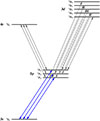 |
Fig. 1. Energy level diagram of the atomic model of the O I IR triplet adopted in this work. Blue arrows indicate the transitions of the O I IR triplet, while gray arrows represent the other radiative transitions included in the model. |
The scattering polarization of the O I IR triplet is the observational signature of atomic alignment, quantified by the  multipole components of the density matrix (see, e.g., Landi Degl’Innocenti & Landolfi 2004, for details on the physical link between alignment and polarization). Once these components are determined, the emergent fractional linear polarization Q/I can be obtained from the standard relations that connect it to the degree of alignment (e.g., Trujillo Bueno 1999; Derouich et al. 2007). It is worth noting that these approximate relations were derived for 90° scattering in an optically thin slab. They are widely used for trend and sensitivity analyses (e.g., Belluzzi et al. 2009; Belluzzi & Trujillo Bueno 2011, including Ca II H&K, Mg II h&k, Na I D1&D2, and O I 777 nm). In the future, a more quantitative study will require full non-LTE radiative transfer synthesis.
In addition to radiative rates associated with emission and absorption processes, we include two other main contributions in modeling the formation and polarization of the O I IR triplet lines: isotropic collisions with neutral hydrogen atoms and the Hanle effect due to a turbulent magnetic field. The radiative contribution to the SEE adopted in this study follows the formalism of Landi Degl’Innocenti & Landolfi (2004), within the framework of the so-called multilevel atom in the tensorial basis.
In the numerical implementation, the contribution of the incident radiation field is specified through the anisotropy factor, defined as  , and the number of photons per mode, given by
  . These quantities are evaluated following the method described by Manso Sainz & Landi Degl’Innocenti (2002) based on the data given by Cox (2000). The Einstein coefficients required for the radiative rates entering the SEE are extracted from the NIST database.
In the following sections, we describe the inclusion of the magnetic and collisional contributions in the SEE.
3. Magnetic contribution
Adopting a frame whose quantization axis is aligned with the symmetry axis of the radiation field, the Hanle effect of a magnetic-field on the irreducible density–matrix components ρqk𝒥(α 𝒥) is given by (e.g., Landi Degl’Innocenti et al. 1990)
 (1)
(1)
where
-
ωL is the Larmor frequency, proportional to the magnetic-field strength B;
-
g𝒥 is the Landé factor of level (α𝒥);
-
 is the magnetic kernel that couples components with different q and accounts for the rotation from the magnetic frame (quantization axis along B) to the chosen reference frame (see Landi Degl’Innocenti et al. 1990).
All radiative rates entering the SEE are formally invariant under rotations of the reference frame (e.g., Landi Degl’Innocenti & Landolfi 2004).
When the magnetic field is turbulent, it is appropriate to average the effect of the magnetic field over all possible orientations. The angle-averaged density matrix component is
 (2)
(2)
This integral accounts for all possible magnetic field directions (θB, χB), assuming a constant field strength B, where θB is the inclination angle with respect to the quantization axis and χB is the azimuthal angle measured in the plane perpendicular to that axis. With unpolarized, axially symmetric illumination and an isotropically distributed (turbulent) magnetic field, the q ≠ 0 coherences cannot be produced, leaving only the azimuthally invariant q = 0 components (independent of χB). By using the change of variables μB = cos θB, Equation (2) becomes
 (3)
(3)
ρ0k(J; μB) is the solution of the SEE for a given direction of the magnetic field, characterized by the inclination θB (since it is independent of χB). The averaging over θB ∈ [0, π] ensures isotropy of the field. This treatment implicitly assumes that the magnetic field strength is constant but its direction is random. The averaging over θB is carried out using a Gaussian quadrature with N = 15 points, which provides accurate convergence. For the sake of simplicity, in Sections 5 and 6, we denote the isotropic-field-averaged density matrix element  simply as ρ0k𝒥(α 𝒥).
4. Collisional contribution in the multilevel case
4.1. SEE collisional contribution
In the tensorial basis, the contribution of depolarizing isotropic collisions to the SEE is given by (e.g., Sahal-Bréchot et al. 2007)
 (4)
(4)
where 0 ≤ k𝒥 ≤ k𝒥,max with k𝒥, max = 2𝒥 for 𝒥 = 𝒥′ and k𝒥, max = min{2𝒥, 2𝒥′} for 𝒥 ≠ 𝒥′. Here Dk(α 𝒥, T) and Dk(α 𝒥 → α 𝒥′,T) are the depolarization and the polarization transfer rates, respectively. Note that D0(α 𝒥, T) = 0 by definition and that D0(α 𝒥 → α 𝒥′,T) is the population transfer rate between the levels (α 𝒥) and (α 𝒥′). These rates should be calculated independently.
4.2. Collisional rates calculation
To calculate the depolarization and transfer of polarization rates for levels of complex atoms, Derouich et al. (2005b) proposed a collisional method based on the frozen core approximation (see also Derouich 2020). In the framework of this method, the complex atom is assumed to be composed of the following:
-
Electrons in an internal subshell where their total orbital momentum is zero.
-
Outer incomplete (open) shell containing electrons with nonzero total orbital momentum denoted as Lc and a total spin Sc. This shell is called the core of the complex atom.
-
An optical electron with orbital angular momentum l and spin s (
 ).
).
We use the following coupling scheme to obtain the total angular momentum 𝒥:

where:
-
l and s are the orbital and spin angular momenta of the valence electron (l and s are the corresponding quantum numbers),
-
j is the total angular momentum of the optical electron (j is the corresponding quantum number),
-
Lc and Sc are the total orbital and spin angular momenta of the core (Lc and Sc are the corresponding quantum numbers),
-
Jc is the total angular momentum of the core (Jc is the corresponding quantum number),
-
𝒥 is the total angular momentum of the complex atom which is here the O I (𝒥 is the corresponding quantum number).
We assume that only the valence electron is affected by the interaction with neutral hydrogen atoms. The electrons of the core are considered to not be influenced by the collisions, in the sense that Lc, Sc, and Lc = Sc + Sc are conserved under the frozen core approximation. Therefore, the polarization transfer rates Dk𝒥(α 𝒥′→α 𝒥, T) are given by the following linear combination of the rates of simple atoms Dkj(j → j′) (see Nienhuis 1976; Omont 1977; Derouich 2020):
 (5)
(5)
and, for the depolarization rates, one has
 (6)
(6)
The atomic model of the O I adopted in this work involves levels where the orbital momentum of the valence electron is l = 0, 1, or 2. Rates Dkj(j → j′) and Dkj(j) for the cases where l = 1 or 2 (i.e., p- and d-states) are tabulated in the form of variation laws for all orders kj in Derouich (2020). For l = 0, Dkj(j) are also available in the form of variation laws for all s-states in Derouich et al. (2005a). These variation laws depend on the effective quantum number n*, which must be calculated for all levels involved in the atomic model. Once n* is determined, the corresponding Dkj(j → j′) and Dkj(j) rates can be obtained, and subsequently used to calculate the rates Dk𝒥(α 𝒥 → α 𝒥′) and Dk𝒥(α 𝒥) of the O I atoms due to collisions with hydrogen atoms. Recall that, if the energy of the level of interest is denoted by Elevel, and the ionization energy of the perturbed atom in its fundamental state is E∞, then the effective quantum number is given by
![Mathematical equation: $$ \begin{aligned}n^{*}=[2(E_{\infty }-E_{\rm level})]^{-1/2} \, ,\end{aligned} $$](/articles/aa/full_html/2026/01/aa56214-25/aa56214-25-eq15.gif)
where both E∞ and Elevel are expressed in atomic units.
Following the procedure outlined above, we calculate the rates Dk𝒥(α 𝒥) and Dk𝒥(α 𝒥 → α 𝒥′), and express them in the following form
 (7)
(7)
The coefficients ak𝒥, corresponding to depolarization and polarization transfer rates, are listed in Tables A.1 and A.2 of Appendix A, respectively, for all levels of the model of O I IR triplet under consideration and for all even orders k𝒥1. As explained in Derouich et al. (2005a) and in Derouich (2020), λk𝒥 can be approximated by 0.416 for s-states and by 0.38 for p- and d-states. We specify that the adopted Dk𝒥 rates are calculated in the absence of magnetic fields (i.e., zero-field rates), which should be a good approximation under the Hanle-effect regime field strengths considered here, since the impact of the field on the interaction potential is expected to be weak and 𝒥 remains a good quantum number (see Derouich & Qutub 2024, for details).
It is worth noting that radiative rates are taken from available databases where they are usually computed within the L-S coupling scheme, whereas collisional rates are calculated using a different angular momentum coupling. Although the two coupling schemes are not formally identical, this mixed approach is common practice and allows us to make use of the best available data for both radiative and collisional processes.
5. Results and discussion
5.1. Effect of collisions
Using the multilevel atomic model for O I IR triplet shown in Figure 1, we solve the SEE to compute the nonzero components ρ0k𝒥 in the presence of a turbulent magnetic field. The numerical code incorporates the collisional rates given by Equation (7) with the values of the ak𝒥 coefficient provided in Tables A.1 and A.2 as inputs, along with an anisotropic radiation field characterized by J00(ν) and J02(ν). These computations are performed over a wide range of hydrogen density, from 1011 cm−3 to 1019 cm−3, assuming a solar temperature of T = 5000 K, and magnetic field strengths in the range 1 mG to 100 G.
Since collisional rates are proportional to the hydrogen density nH, as per the impact approximation, studying the effect of collisions on polarization is effectively equivalent to analyzing its dependence on nH. Figure 2 illustrates the normalized atomic alignment [ρ0(2)(nH)/ρ0(2)(nH = 0)]B = 0 as a function of the hydrogen density nH for each of the four fine-structure levels involved in the O I IR triplet: the upper levels 3p 5P1 (blue curve), 3p 5P2 (red curve), 3p 5P3 (brown curve), and the lower level 3s 5S2 (black curve). The figure shows that all levels begin to be sensitive to elastic collisions with neutral hydrogen for nH ≳ 1014 cm−3. Among them, the 3s 5S2 level depolarizes more rapidly than the upper levels, becoming almost completely depolarized around nH ∼ 1016 cm−3, which is typical of photospheric conditions. In contrast, at chromospheric densities (nH ∼ 1014 cm−3), its alignment is only slightly affected by collisions.
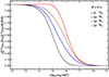 |
Fig. 2. Normalized atomic alignment [ρ0(2)(nH)/ρ0(2)(nH = 0)]B = 0 as a function of hydrogen density nH in the absence of a magnetic field (B = 0), showing the pure effect of elastic collisions on the fine-structure levels of the O I IR triplet. |
Focusing on the upper levels, the state 3p 5P2 retains its alignment more effectively than the states 3p 5P1 and 3p 5P3, maintaining approximately 70% of its alignment even at nH ∼ 1016 cm−3. By comparison, the alignment of 3p 5P1 (the most sensitive to depolarizing collisions among the upper levels) and 3p 5P3 decreases more rapidly with increasing nH, though remains noticeable even at nH ∼ 1016 cm−3. Thus, in the absence of magnetic fields, the upper levels of O I IR lines (especially 3p 5P2) remain polarized at photospheric densities (nH ∼ 1015–1016 cm−3), as shown in Figure 2.
To explore the impact of large uncertainties, which may arise from the use of rough approximations in calculating the elastic collisional rates for collisions between hydrogen and oxygen atoms, we have tested the effect of increasing or decreasing the rates by one order of magnitude. Here, D denotes the total depolarizing effect of elastic H–O collisions, represented by the complete set of depolarization and polarization transfer rates listed in Tables A.1 and A.2. We express the results as the percentage variation of the alignment relative to the reference case (1 × D), obtained by either decreasing the rates by a factor of 10 (D/10) or increasing them by a factor of 10 (10 × D). These percentage variations can take both negative and positive values, depending on whether the alignment decreases or increases relative to the reference case. At nH = 1015 cm−3, the alignment of the 3s5S2 level changes from −84.7% (D/10) to +87.4% (10 × D), while the alignment of the 3p3P1 level varies from −40.0% to +60.1%. At 1016 cm−3, the discrepancies become even larger, reaching −692.7% and +97.4% for the 3s5S2 level, and −150.4% and +81.5% for the 3p3P1 level. At 1017 cm−3, where the alignment of 3s5S2 is already very small, the deviations are extreme, with the 3s5S2 level ranging from −3816.6% to +98.8% and the 3p3P1 level from −440.2% to +88.9%. Figure 3 illustrates the results. We also performed the same analysis for the other two upper levels of the triplet, 3p3P2 and 3p3P3, and found analogous results. This suggests that the O I IR triplet polarization is highly sensitive to the adopted collisional rates.
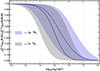 |
Fig. 3. Sensitivity of the normalized alignment, |

5.2. Interplay between collisions and magnetic fields
To assess the joint influence of the turbulent magnetic field and collisions on the atomic alignment of the O I levels, we compute the normalized atomic alignment ρ0(2)(nH, B)/ρ0(2)(nH, B = 0) as a function of the magnetic field strength B, for various fixed hydrogen densities nH. The results for 3p 5P1, 3p 5P2, 3p 5P3, and 3s 5S2 levels, presented in Figure 4, show that the magnetic field plays a significant role in depolarizing the levels involved in the formation of the IR triplet. This highlights the interplay between the Hanle effect and elastic collisions in shaping the polarization signals.
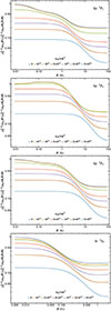 |
Fig. 4. Normalized alignment, ρ0(2)(nH, B)/ρ0(2)(nH = 0, B = 0), as a function of the magnetic field strength B for several hydrogen densities nH, for four levels of O I. From top to bottom: 3p 5P1, 3p 5P2, 3p 5P3, and 3s 5S2. Each curve corresponds to a fixed value of nH, ranging from 0 to 5 × 1016 cm−3, as labeled. The plots illustrate how both elastic collisions with neutral hydrogen and the Hanle effect contribute to the depolarization of each level. |
The top three panels of Figure 4 correspond to the upper levels of the IR triplet: 3p 5P1, 3p 5P2, and 3p 5P3, while the bottom panel corresponds to the lower level 3s 5S2. Each curve in the plots represents a different hydrogen density, ranging from nH = 0 to 5 × 1016 cm−3. Across all levels, the alignment decreases almost monotonically with increasing B and nH, reflecting the progressive depolarization induced by elastic collisions and the Hanle effect.
The 3s 5S2 level is the most sensitive to depolarizing mechanisms: for nH ∼ 1016 cm−3 and B ∼ 20 G, its alignment is almost entirely suppressed. Among the upper levels, 3p5P1 is the most sensitive to magnetic depolarization, with a rapid decline in alignment for B ≳ 1 G when nH ≳ 1015 cm−3. In contrast, the alignment of level 3p5P3 declines a bit more gradually, indicating moderately lower sensitivity to weak fields, and it is also less affected by collisional depolarization compared to 3p5P1. The alignment of level 3p 5P2 is the most resistant among the upper levels, retaining a significant fraction of its alignment at nH ≲ 5 × 1015 cm−3 and B ≲ 10 G. It is also noteworthy that the magnetic field strength at which polarization is most sensitive shifts to higher values with increasing hydrogen density nH, indicating a coupled dependence on both collisional and magnetic depolarization mechanisms.
Complementing this analysis, Figure 5 shows the normalized atomic alignment, defined as ρ02(nH, B)/ρ02(nH = 0, B = 0), as a function of hydrogen density for the same four O I levels for a magnetic field strength of B = 20 G. This quantity captures how collisional and magnetic depolarization, acting together, reduce the alignment relative to the undisturbed case. The lower level 3s 5S2 (black curve) depolarizes the fastest and most significantly: at the photospheric density nH ∼ 1015 cm−3 and for a magnetic field strength of B = 20 G, its alignment is practically zero. The alignment of the upper levels, 3p 5P1 (blue curve), 3p 5P2 (red curve), and 3p 5P3 (brown curve), is reduced by approximately 90% at nH ∼ 1016 cm−3 and B = 20 G. Stronger magnetic fields (B > 20 G) cause alignment to decay even more rapidly (see Figure 4), highlighting the combined depolarizing effects of the Hanle effect and collisions.
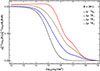 |
Fig. 5. Same as Figure 2, but for a magnetic field strength of B = 20 G, illustrating the combined effect of elastic collisions and magnetic depolarization (Hanle effect) on the atomic alignment of the O I IR triplet levels. |
Our analysis shows that incorporating collisional rates computed for photospheric hydrogen densities and a quiet-Sun turbulent magnetic field near the Hanle saturation regime into the SEE strongly suppresses atomic alignment. This contrasts with the conclusion of del Pino Alemán & Trujillo Bueno (2015, 2017), who reported that the bulk of the polarization is destroyed in the photosphere, even under the action of very weak magnetic fields, well before the saturation regime is reached. A possible reason for this discrepancy is that their modeling relied on overestimated inelastic collisional rates that contribute to depolarization (whereas in our case they are negligible). In practice, this would means that part of the depolarization attributed in our work to the Hanle effect was, in their case, effectively taken up by inelastic collisions. Overestimating the impact of inelastic collisions, thus, would reduce the magnetic field strengths required in their modeling, and this may have been compounded by their use of an approximate treatment of elastic collisions.
The rapid loss of alignment at nH ≳ 1015 cm−3, under magnetic field strengths typical of the quiet-Sun, confirms that a significant contribution to the polarization of the IR triplet should primarily originate in higher chromospheric layers (see also del Pino Alemán & Trujillo Bueno 2015, 2017), where hydrogen densities are lower and collisional depolarization is weaker. In the future, it will be of great interest to incorporate accurate collisional depolarization rates into realistic non-LTE radiative transfer calculations.
6. Solar implications and conclusions
Our study provides insights into the expected roles of elastic and inelastic collisions and turbulent magnetic fields in the formation and observability of the scattering polarization signals of the O I IR triplet in the solar atmosphere.
In the solar photosphere, where hydrogen densities are typically nH ∼ 1015 − 1016 cm−3, collisions alone lead to a substantial reduction of alignment, particularly for the lower level 3s 5S2 and the upper level 3p 5P1. Among the upper levels, 5P2 is found to retain the highest alignment. The inclusion of a turbulent magnetic field with strength B ∼ 20 G further enhances this depolarization, leading to suppression levels above 90% for most levels. Conversely, in the upper chromosphere, where nH ≲ 1014 cm−3, collisional depolarization becomes inefficient; even in the presence of magnetic fields, a residual atomic alignment can persist and may be sufficient to produce measurable Q/I signals (see also del Pino Alemán & Trujillo Bueno 2015, 2017).
These results highlight the importance of an accurate treatment of both collisional and magnetic depolarization mechanisms in non-LTE radiative transfer models to ensure accurate magnetic diagnostics based on the Hanle effect. The O I IR triplet remains a valuable probe of chromospheric magnetism, provided that the relevant physical processes are fully taken into account.
Recall that odd orders of k are not relevant in the present context, as only linear polarization is considered in this study.
Acknowledgments
This research work was funded by Institutional Fund Projects under grant no. (IFPIP:52-130-1443). The authors gratefully acknowledge technical and financial support provided by the Ministry of Education and King Abdulaziz University, DSR, Jeddah, Saudi Arabia.
References
- Asplund, M., Amarsi, A. M., & Grevesse, N. 2021, A&A, 653, A141 [NASA ADS] [CrossRef] [EDP Sciences] [Google Scholar]
- Barklem, P. S. 2007, A&A, 462, 781 [NASA ADS] [CrossRef] [EDP Sciences] [Google Scholar]
- Belluzzi, L., & Trujillo Bueno, J. 2011, ApJ, 743, 3 [NASA ADS] [CrossRef] [Google Scholar]
- Belluzzi, L., Landi Degl’Innocenti, E., & Trujillo Bueno, J. 2009, ApJ, 705, 218 [Google Scholar]
- Cox, A. N. 2000, Allen’s Astrophysical Quantities (New York: Springer) [Google Scholar]
- del Pino Alemán, T., & Trujillo Bueno, J. 2015, ApJ, 808, L13 [Google Scholar]
- del Pino Alemán, T., & Trujillo Bueno, J. 2017, ApJ, 838, 164 [Google Scholar]
- Derouich, M. 2020, ApJS, 247, 72 [NASA ADS] [CrossRef] [Google Scholar]
- Derouich, M., & Qutub, S. 2024, A&A, 683, A173 [NASA ADS] [CrossRef] [EDP Sciences] [Google Scholar]
- Derouich, M., Barklem, P. S., & Sahal-Bréchot, S. 2005a, A&A, 441, 395 [NASA ADS] [CrossRef] [EDP Sciences] [Google Scholar]
- Derouich, M., Sahal-Bréchot, S., & Barklem, P. S. 2005b, A&A, 434, 779 [NASA ADS] [CrossRef] [EDP Sciences] [Google Scholar]
- Derouich, M., Trujillo Bueno, J., & Manso Sainz, R. 2007, A&A, 472, 269 [NASA ADS] [CrossRef] [EDP Sciences] [Google Scholar]
- Fontenla, J. M., Avrett, E. H., & Loeser, R. 1993, ApJ, 406, 319 [Google Scholar]
- Keller, C. U., & Sheeley, N. R. 1999, in Scattering Polarization in the Chromosphere, eds. K. N. Nagendra, & J. O. Stenflo (Dordrecht: Springer), 17 [Google Scholar]
- Landi Degl’Innocenti, E., & Landolfi, M. 2004, Polarization in Spectral Lines,, 307 (Dordrecht: Sprintger) [Google Scholar]
- Landi Degl’Innocenti, E., Bommier, V., & Sahal-Brechot, S. 1990, A&A, 235, 459 [Google Scholar]
- Manso Sainz, R., & Landi Degl’Innocenti, E. 2002, A&A, 394, 1093 [NASA ADS] [CrossRef] [EDP Sciences] [Google Scholar]
- Nienhuis, G. 1976, J. Phys. B Atomic Molecul. Phys., 9, 167 [Google Scholar]
- Omont, A. 1977, Progr. Quant. Electr., 5, 69 [Google Scholar]
- Sahal-Brechot, S. 1977, ApJ, 213, 887 [Google Scholar]
- Sahal-Bréchot, S., Derouich, M., Bommier, V., & Barklem, P. S. 2007, A&A, 465, 667 [NASA ADS] [CrossRef] [EDP Sciences] [Google Scholar]
- Sheeley, N. R., Jr, & Keller, C. U. 2003, ApJ, 594, 1085 [Google Scholar]
- Stenflo, J. 1994, Solar Magnetic Fields: Polarized Radiation Diagnostics, 189 [Google Scholar]
- Trujillo Bueno, J. 1999, in Polarization, eds. K. N. Nagendra, & J. O. Stenflo, Astrophysics and Space Science Library, 243, 73 [Google Scholar]
- Trujillo Bueno, J. 2001, in Advanced Solar Polarimetry - Theory, Observation, and Instrumentation, ed. M. Sigwarth, ASP Conf. Ser., 236, 161 [NASA ADS] [Google Scholar]
- Trujillo Bueno, J., Collados, M., Paletou, F., & Molodij, G. 2001, in Advanced Solar Polarimetry - Theory, Observation, and Instrumentation, ed. M. Sigwarth, ASP Conf. Ser., 236, 141 [NASA ADS] [Google Scholar]
Appendix A: Collisional data
O Inonzero collisional depolarization ratesDk𝒥(α 𝒥) for the multilevel case.
O Icollisional depolarization ratesDk𝒥(α 𝒥 → α 𝒥′) for the multilevel case.
All Tables
All Figures
|
Fig. 1. Energy level diagram of the atomic model of the O I IR triplet adopted in this work. Blue arrows indicate the transitions of the O I IR triplet, while gray arrows represent the other radiative transitions included in the model. |
| In the text | |
|
Fig. 2. Normalized atomic alignment [ρ0(2)(nH)/ρ0(2)(nH = 0)]B = 0 as a function of hydrogen density nH in the absence of a magnetic field (B = 0), showing the pure effect of elastic collisions on the fine-structure levels of the O I IR triplet. |
| In the text | |
|
Fig. 3. Sensitivity of the normalized alignment, |
| In the text | |
|
Fig. 4. Normalized alignment, ρ0(2)(nH, B)/ρ0(2)(nH = 0, B = 0), as a function of the magnetic field strength B for several hydrogen densities nH, for four levels of O I. From top to bottom: 3p 5P1, 3p 5P2, 3p 5P3, and 3s 5S2. Each curve corresponds to a fixed value of nH, ranging from 0 to 5 × 1016 cm−3, as labeled. The plots illustrate how both elastic collisions with neutral hydrogen and the Hanle effect contribute to the depolarization of each level. |
| In the text | |
|
Fig. 5. Same as Figure 2, but for a magnetic field strength of B = 20 G, illustrating the combined effect of elastic collisions and magnetic depolarization (Hanle effect) on the atomic alignment of the O I IR triplet levels. |
| In the text | |
Current usage metrics show cumulative count of Article Views (full-text article views including HTML views, PDF and ePub downloads, according to the available data) and Abstracts Views on Vision4Press platform.
Data correspond to usage on the plateform after 2015. The current usage metrics is available 48-96 hours after online publication and is updated daily on week days.
Initial download of the metrics may take a while.