| Issue |
A&A
Volume 705, January 2026
|
|
|---|---|---|
| Article Number | A57 | |
| Number of page(s) | 13 | |
| Section | Galactic structure, stellar clusters and populations | |
| DOI | https://doi.org/10.1051/0004-6361/202556408 | |
| Published online | 07 January 2026 | |
The Gaia-ESO survey: Open clusters as tracers of galactic chemical evolution
1
School of Physical and Chemical Sciences, University of Canterbury,
Kirkwood Ave,
Canterbury,
New Zealand
2
Institute of Astronomy, University of Cambridge,
Madingley Road,
Cambridge CB3 0HA,
UK
3
Institute of Theoretical Physics and Astronomy, Faculty of Physics, Vilnius University,
Sauletekio av. 3,
10257
Vilnius,
Lithuania
4
INAF – Osservatorio Astrofisico di Arcetri, Largo E. Fermi,
5,
50125
Firenze,
Italy
5
INAF – Osservatorio di Astrofisica e Scienza dello Spazio,
via P. Gobetti 93/3,
40129
Bologna,
Italy
6
Lund Observatory, Division of Astrophysics, Department of Physics, Lund University,
Box 118,
22100
Lund,
Sweden
7
Centro de Astrobiología, CSIC-INTA,
Camino bajo del castillo s/n, 28692, Villanueva de la Canãda,
Madrid,
Spain
8
School of Physics, University of New South Wales,
Sydney, NSW,
Australia
9
INAF – Osservatorio Astronomico di Palermo,
Piazza del Parlamento 1,
90134
Palermo,
Italy
★ Corresponding author: This email address is being protected from spambots. You need JavaScript enabled to view it.
Received:
14
July
2025
Accepted:
14
October
2025
Abstract
Aims. We investigate the formation and evolutionary trajectory of the Milky Way’s inner and outer galactic regions using stars from open clusters in the Gaia-ESO OC survey.
Methods. Using numerical simulations from Chempy, we leveraged Markov chain Monte Carlo sampling techniques to derive galactic evolutionary parameters for each open cluster by fitting measured abundances of elements C, N, O, Mg, Si, Ca, Ti, Fe, Mn, Zn, Y, and Ba.
Results. We find differing evolutionary histories between the inner and outer regions of the Milky Way that align with variations in the slope of the initial mass function, the rate of Type Ia supernovae, and the galactic metallicity gradient traced by open clusters.
Conclusions. Our results support established galactic formation and evolutionary theories, highlighting that the inner Galaxy had a short and intense early star formation epoch followed by reduced activity. In contrast, the outer Galaxy maintained a more sustained star formation history.
Key words: Galaxy: evolution / Galaxy: formation / open clusters and associations: general
© The Authors 2026
 Open Access article, published by EDP Sciences, under the terms of the Creative Commons Attribution License (https://creativecommons.org/licenses/by/4.0), which permits unrestricted use, distribution, and reproduction in any medium, provided the original work is properly cited.
This article is published in open access under the Subscribe to Open model. This email address is being protected from spambots. You need JavaScript enabled to view it. to support open access publication.
1 Introduction
Galactic chemical evolution (GCE) allows us to probe the formation and evolution of galaxies by studying the chemical compositions of stars at different ages and different locations within the Galaxy (Tinsley & Larson 1978; Timmes et al. 1995; Pagel & Tautvaisiene 1995, 1997; Matteucci 2001; Kobayashi et al. 2006). The key physical processes that determine GCE include the rate of star formation, the initial mass function of stars, and the yield of elements from different enrichment channels. The equations for these parameters are solved numerically to predict the chemical evolution of our Galaxy over time.
However, factors such as stellar age, location, and motion are also important when inferring the history of the Galaxy using GCE (Kroupa & Boily 2002; Martin et al. 2004; Bensby et al. 2005; Roškar et al. 2008; Steinmetz 2012; Prantzos et al. 2023), and there are high uncertainties when determining these values for individual field stars.
Open clusters help reduce these uncertainties. The stars within an open cluster are co-eval (Lada & Lada 2003), and as they formed from the same gas cloud, they are chemically homogeneous (Poovelil et al. 2020). Therefore, age, distance, and chemical signature can be determined for each cluster with a better accuracy than for single stars in the field (Magrini & Randich 2014). Additionally, open clusters can be found at a range of ages, allowing galactic evolution to be tracked across time. Open clusters are generally found within the disc of the Milky Way and typically have metallicities of the thin disc (Elmegreen & Efremov 1997; Joshi 2016; Krause et al. 2020; Piecka & Paunzen 2021).
Open clusters can also be used to quantise the galactic evolutionary parameter space in order to simplify chemical modelling, so they are a valuable tool for studying the chemical evolution of the Milky Way (Strobel 1991; Chen et al. 2003; Frinchaboy et al. 2004; Kharchenko et al. 2005). Applying GCE modelling to an open cluster sample allows the history of chemical enrichment at the location of each cluster prior to its formation to be inferred (Sestito et al. 2006; Bragaglia et al. 2008; Sestito et al. 2008; Stanghellini & Haywood 2010; Reddy et al. 2020).
In this study, we use the open cluster sample within the Gaia-ESO survey (GES: Gilmore et al. 2022; Randich et al. 2022) to investigate the formation and evolutionary history of the Milky Way in the inner and outer galactic regions of the disc. We modelled the GCE using Chempy (Rybizki et al. 2017), which is described further in Sect. 3. The GES open cluster sample was designed to provide an unbiased and comprehensive set of open clusters with which to investigate the open cluster system of the Milky Way (Randich et al. 2022). In particular, the selection was optimised in age, metallicity, galactocentric radial distance, and mass, and it captures most phases of evolution with ages between 1 Myr and 8 Gyr. GES observed 40304 stars across 62 clusters and extracted further data from the ESO archive, adding 1740 stars across another 18 clusters. (See Bragaglia et al. (2022); Blomme et al. (2022) for further details.)
The GCE code Chempy (Rybizki et al. 2017) is a one-zone chemical evolution model. The one-zone model treats the entire galaxy as a single instantaneously well-mixed ‘zone’ of gas, where all the gas and stars have the same starting chemical composition and evolve simultaneously over time. This model is inherently inaccurate in modelling complex environments such as the Milky Way. However, we reduced the impact of the onezone model’s inaccuracy by assuming each open cluster is born from a unique molecular cloud within the Milky Way, allowing us to model each open cluster as a single isolated zone that is part of a complex multi-zone system.
This paper is structured as follows. In Section 2 we detail the methodology used in selecting the open cluster sample and an investigation into the dataset. Section 3 provides an outline of the chemical evolution modelling framework, including assumptions, input yields, and computational techniques. In Sect. 4, we evaluate the open cluster results of each evolutionary parameter that governs the model’s behaviour. Section 5 provides a general discussion of the findings, and in Sect. 6 we summarise the results and key conclusions.
2 Data
The Gaia-ESO survey included a Milky Way field science programme (Gilmore et al. 2022) and calibration star programme (Pancino et al. 2017) alongside the open cluster science programme (Randich et al. 2022). Observations were made using FLAMES (Pasquini et al. 2002) on the ESO very large telescope (VLT), for which fibres to both GIRAFFE (R ∼ 18 000) and UVES (R ∼ 47 000) spectrographs were employed. All data were processed by dedicated data reduction pipelines for each instrument (Gilmore et al. 2022), and a range of analysis teams extracted stellar parameters, chemical abundances, and other stellar measurements for both the medium and high resolution spectra. These results were first homogenised by instrument (Smiljanic et al. 2014; Worley et al. 2024) and then placed into a single star catalogue (Hourihane et al. 2023).
2.1 Open cluster member selection
The sample of open clusters was taken from the GaiaESO (GES) DR5 dataset (Randich et al. 2022) with GES_TYPE=*_OC. It was then reduced to stars in the temperature range 3000 K ≤ Teff ≤ 7000 K.
The cluster members were selected using the membership probability (column ‘MEM3D’) calculated through astrometric analysis of the GES open clusters carried out in Jackson et al. (2021). The targets selected for the GES open cluster program were split into two observation resolutions (Bragaglia et al. 2022). The first group of targets were observed at medium resolution (R ∼ 18 000) using GIRAFFE and represent a large unbiased selection. The second group of targets were observed using UVES at high resolution (R ∼ 47 000) and represent a smaller selection of only high-probability open cluster members. We utilised stars from both groups but selected only those stars with a probability greater than 70% of being cluster members. This filter removed 71% of the stars.
We then needed to ‘clean’ the GES dataset to select only high-quality observations with low uncertainties. We also considered the completeness of the chemical elements that have been measured among the open cluster members to ensure that our chemical evolution code uses a similar complete set of observational constraints.
First, we required each star to have at least three abundance measurements to be included in our final sample to ensure a more complete set of abundances. We did this because one of the science goals of GES was to measure the lithium abundance of as many stars as possible, particularly for open cluster stars. The GES dataset has many stars that only have iron and lithium abundances that have been calculated and no other abundances. This step removed 58% of the remaining stars.
We then removed low signal-to-noise (S/N) observations. A high S/N is crucial in spectroscopy, as it enhances the measurement of spectral features, allowing for accurate determination of stellar properties, including chemical abundances. We selected only measurements that have an S/N above 20. The S/N threshold removed 15% of the remaining stars.
The final sample contains 3379 (10.42%) of the initial 32 440 stars. Table 1 shows the exact number of stars removed at each cleaning stage, starting from the raw dataset.
Figure 1 shows a Kiel diagram of all the GES DR5 stars (within our temperature range) in the open cluster survey before cleaning (grey) and after applying the above cleaning criteria (blue). The final selection covers a broad range of log g and Teff, allowing us to trace the parameter space of the GES sample.
Gaia-ESO sample member selection.
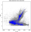 |
Fig. 1 Sample selection from the Gaia-ESO DR5 open cluster dataset. The base dataset is shown in grey, and the selected data after processing and cleaning are shown in blue. |
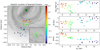 |
Fig. 2 Final sample of open cluster stars. Left: galactic location of the open clusters, where the dark-green dotted circle and solid circle denote the solar radius and the galactic centre, respectively. The inset shows a closer view of the clusters in the solar neighbourhood. Right: open cluster ages (top), height above the Galactic plane (middle), and metallicity [Fe/H] (bottom), each against galactocentric radius. The colour map of [Fe/H] is the same for all four plots.} |
2.2 Open cluster distribution
The entire GES open cluster set had 80 clusters that we reduced to a final selection of 48 clusters after the cleaning. For each cluster, we attributed a cluster abundance and uncertainty by selecting the median abundance and mean absolute deviation of the cluster members that remain after the data cleaning process. The use of the median values reduced the impact of remaining outliers in a cluster’s members. Figure 2 displays our final selection of open clusters, and details on each cluster’s primary properties as calculated by Randich et al. (2022) can be found in Table C.1.
The left plot shows the locations of the open clusters within the Milky Way, while the three plots on the right display some key properties against their galactocentric radius. The colour map of [Fe/H] is the same for all four plots. The top-right plot shows the age of the open clusters, in which we noticed that the solar neighbourhood (∼ 8 Rgc) has a large spread in age covering the youngest clusters (∼ 0.01 Gyr) and intermediate age clusters (up to ∼ 1 Gyr). We expected this to provide more information to deduce the evolution of chemical elements in this region. The outer Galaxy contains mostly old clusters >1 Gyr. The middle-right plot shows the height above the Galactic plane, which has an increasing trend with increasing radius. Many of the open clusters in the outer Galaxy are |Z|>100 pc. The bottom-right plot shows the metallicity [Fe/H] gradient of the Milky Way as traced by the open clusters. There is also a noticeable flattening of the gradient from a radius of ∼ 10 kpc. This is a well-known feature of open clusters (Magrini et al. 2009; Reddy et al. 2016; Spina et al. 2022; Magrini et al. 2023). We also note that there is a gap in the data between ∼ 8.5 kpc and ∼ 10 kpc. This is the fairly empty region between the Sun (in the Orion Spur) and the outer spiral arm (Perseus).
2.3 Element selection
The Gaia-ESO survey measured 30+ elements in various quantities across the cluster members. Some stars may have only 12 of the 30+ elements available, while other may have all 30+ available. We selected elements to use in the simulations that characteristically represented the different nucleosynthesis channels. The Chempy GCE simulation is configured to model different nucleosynthesis channels: Big Bang nucleosynthesis; Type Ia supernova (SN Ia); Type II supernova (SN II), including 50% exploding as hypernova; asymptotic giant branch (AGB) stars; and nucleosynthesis via general stellar evolution.
The initial state of our simulation starts with a pure cloud of hydrogen (H) and helium (He) gas synthesised from Big Bang nucleosynthesis. Thus, H and He are required in the simulation and are traced by Chempy. Magnesium (Mg I), oxygen (O I), and silicon (Si I) are mainly produced in SN II, while calcium (Ca I) and titanium (Ti I) are thought to be produced in approximately equal parts from SN II and SN Ia (Kobayashi et al. 2020). Iron (Fe) and manganese (Mn I) are produced primarily from SN Ia (Kobayashi et al. 2020; Ting & Weinberg 2022), though with a non-negligible contribution from SN II. Carbon (C I) and nitrogen (N derived from the CN molecule) trace the main sequence and red giant stellar evolution. Zinc (Zn I) was chosen as the characteristic hypernova element (Kobayashi et al. 2020). Finally, we chose Yttrium (Y II) as the light s-process and Barium (Ba II) as the heavy s-process element produced in AGB stars (Karakas et al. 2007).
Modelling of the r-process production sites such as neutron star mergers (NSMs) and magneto-rotational supernovae (MRSNe) are not included in the version of Chempy we used. Because of this, we could not include any element that includes contributions from the r-process. For example, neodymium is produced from approximately 56% s-process and 44% r-process at solar metallicity (Battistini & Bensby 2016), but as r-process channels are not included in the model, the GCE model will attempt to produce the entirety of the neodymium abundance purely from s-process AGB nucleosynthesis, thus biasing the results towards a model that has an over-abundance of AGBs contributing to the chemical evolution of the Galaxy. The final set of elements used in our simulations includes carbon (C), nitrogen (N), oxygen (O), magnesium (Mg), silicon (Si), calcium (Ca), titanium (Ti), iron (Fe), manganese (Mn), zinc (Zn), yttrium (Y), and barium (Ba).
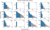 |
Fig. 3 Uncertainty distribution of abundance measurements from the GES DR5 open cluster dataset before (grey) and after (blue) the percentile filter was applied. |
2.4 Abundance uncertainty distributions
Based on inspection of the full GES medium resolution dataset in Figure 16 of Worley et al. (2024), the highest quality results (those based on multiple analyses) typically have uncertainties within 0.5 dex. Some elements, such as Si, Ca, Ti, Y, and Ba used here, have extended distributions greater than 0.5 dex. Using this as a preliminary threshold (note also our criterion of S/N>20 in Table 1), for the elements analysed here, we applied a percentile filter to limit the maximum uncertainty to be below approximately 0.5 dex, as can be seen in Fig. 3. This allowed us to retain a reasonably sized sample of high-quality abundances while removing those with larger-than-typical uncertainties.
Table 2 lists the key elements, the percentile filter applied, the resulting maximum uncertainty, the number of measurements removed, and the remaining sample of measurements for that element. While we aimed for a maximum of 0.5 dex uncertainty, our process of calculating the required percentile cut, when rounded to the nearest whole number, removed additional measurements that were already below this threshold. The only element that breached the 0.5 dex threshold was Ti as a result of this ‘rounding’ We also note that this abundance cleaning did not reduce any individual star’s total available measurements to below our threshold of three.
The typical dispersion on the central value of our final sample is in the range of 0.04−0.1 dex. This indicates our open clusters are relatively homogeneous (Bovy 2016; Poovelil et al. 2020; Spina et al. 2022).
3 Chemical evolution modelling
Galactic chemical evolution modelling is complicated and involves many parameters (Kobayashi & Nakasato 2011; Matteucci 2021, and references therein). Chemical evolution codes can simplify the calculation by using a model that restricts the parameter space, such as the commonly used ‘one-zone model’ (Talbot & Arnett 1971).
There have been many numerical GCE codes released to the public. Andrews et al. (2017) released flexCE, a flexible one-zone chemical evolution code. Côté et al. (2017); Côté & Ritter (2018), released a one-zone model for the Evolution of GAlaxies (OMEGA) focussing on single stellar populations. Yan et al. (2017) proposed GalIMF, a one-zone model that uses a variable integrated galactic initial mass function. Rybizki et al. (2017) released Chempy, which focuses on parameterised onezone models within a Bayesian framework. Johnson & Weinberg (2020) created a Versatile Integrator for Chemical Evolution (VICE), a well-documented code that uses IMF-averaged yields to reduce computation times for both one-zone and multi-zone models. Additionally, Gjergo et al. (2023) released GalCEM, a modular chemical evolution code that provides detailed results on many chemical isotopes.
These GCE codes generally use a fixed set of evolutionary parameters to run the chemical evolution simulation. We selected Chempy (Rybizki et al. 2017) for its flexible approach to fitting the observed abundance measurements using the Markov chain Monte Carlo (MCMC) algorithm, which marginalises over the free parameters and accounts for configurable yield sets. This approach allowed us to use open clusters as a tracer for GCE by fitting galactic formation parameters to the measured abundances.
We modelled the chemical evolution of each open cluster in the Gaia-ESO dataset using the Chempy GCE code (Rybizki et al. 2017). The Chempy code starts with only hydrogen (H) and helium (He) in the reservoir and evolves to the age of the cluster before terminating. The chemical composition at the stopping time is compared to the observed values, providing a likelihood for the MCMC algorithm to optimise.
Chempy traces the three major enrichment channels of SN Ia, SN II, and AGB stars. The default configuration of Chempy allows stars to explode as SN Ia with a mass in the range of 1 M⊙ ≤ m ≤ 8 M⊙ and as SN II with a mass range of 8 M⊙ ≤ m ≤ 100 M⊙, and we also configured Chempy such that 50% of the SN II more massive than 25 M⊙ explode as hypernova (Kobayashi et al. 2006). Stars may also evolve into an AGB star when they have a mass in the range of 0.5 M⊙ ≤ m ≤ 8 M⊙.
Chempy uses seven parameters. Three are simple stellar population parameters: the high-mass slope of the IMF, the number of SN Ia events, and the delay time distribution for SN Ia events. The remaining four are interstellar medium (ISM) evolution parameters: the peak of the star formation profile, the efficiency of the star formation, the fraction of enriched gas expelled from the ISM, and the size of the initial gas reservoir.
Of these seven parameters that can be inferred by Chempy, we chose to focus on the four most sensitive to the fundamental physical processes parameterised in Chempy. These are the free parameters in our model:
High-mass slope (αIMF) of the Kroupa et al. (1993) initial mass function, which is a power law of the form ξ(m) ∝ mαIMF.
Number of SN Ia per M⊙ per 15 Gyr(NIa) from Maoz et al. (2010).
Peak of the star formation profile (S F Rpeak) of the gammadistribution with the shape of the parameter fixed to k=2.
Efficiency of star formation SFE, defined by Chempy as
 The gamma-distribution used in Chempy to model the star formation rate changes shape based on the S F Rpeak parameter. With a smaller value, the distribution shows a sharp and short peak in the early time of formation, followed by a low rate of star formation for the remainder of the evolution history. However, with a larger value of the S F Rpeak parameter, the shape of the distribution has a later peak and is more sustained throughout the entire evolution history.
The three parameters we do not infer are the SN Ia time delay (τIa) of the delay time distribution (DTD) model of Maoz & Mannucci (2012), the fraction of mass outflowing from the ISM into the reservoir (xout), and the scaling factor of the initial reservoir (fcorona). Our testing with these parameters revealed no changes of these values with the evolution of the MCMC and tended to remain at the mean of the prior. A similar result was found by Blancato et al. (2019).
Table 3 shows the default Gaussian priors and the constraints for all seven parameters. We note that the fixed parameters were selected as the mean of their prior and were unchanging throughout each simulation. These priors and limits were selected from the literature specific to that parameter as they apply to the global Milky Way (refer to Table 1 in Rybizki et al. 2017).
For our fiducial simulation, we selected the default yield tables provided in Chempy for SN II and SN Ia from Nomoto et al. (2013) and Seitenzahl et al. (2013), respectively. For AGB nucleosynthesis, we selected the yields provided by Karakas & Lugaro (2016) so we could include the characteristic s-process element, barium, which is not included in the AGB yields of Karakas (2010) used by default in Chempy.
Each Chempy simulation was run with 100 Myr time intervals per simulation iteration with a maximum time of 13.6 Gyr. The choice of this parameter is known to have a minor effect on the results (Rybizki et al. 2017), but our tests showed it was not enough to significantly change the outcome of our analysis. Chempy terminates the simulation once it reaches the age of the cluster.
The MCMC was run with Nwalkers=20 walkers for a maximum of 1000 iterations, giving an overall maximum of 20 000 samples in the MCMC chain. It is expected that the end section of the MCMC chain is the part that converges about the final value. Thus, the best-fit value was taken as the median value of the converged section of the chain. The upper and lower uncertainty in our fit parameters was taken as the 14th and 86th percentile of the posterior.
To determine if the MCMC chain has converged, we implement the autocorrelation time, τ (Goodman & Weare 2010). For every Niter=100 iterations, we evaluated if the length of the chain was greater than L=100 times the autocorrelation time. We also checked if the change in the autocorrelation time, Δ τ=|τn−L−τn|/τn, between checks was less than d=5%, where τn is the autocorrelation time at the nth iteration. Both of these checks provided a strong indication that the MCMC had converged and was unlikely to change further. The stopping criterion was implemented as
 (1)
where Nwalkers is the number of walkers. The quantity nNwalkers is the current length of the Markov chain. The values Niter, L, and d are configurable within the code. (See Appendix A for further details on the MCMC convergence.)
(1)
where Nwalkers is the number of walkers. The quantity nNwalkers is the current length of the Markov chain. The values Niter, L, and d are configurable within the code. (See Appendix A for further details on the MCMC convergence.)
To validate our choices, we performed tests for the convergence of the MCMC chains, shown in Appendix A; the model accuracy with alternative yield sets, shown in Appendix B; and the model accuracy with an alternative element selection, shown in Appendix C.
Gaia-ESO element abundance cleaning.
Chempy default priors and constraints.
4 Evolutionary parameters
In the following sections, we interpret our results with respect to each of the free parameters in our analysis: IMF high-mass slope, rate of SN Ia, star formation rate, and star formation efficiency. We also discuss the outliers of the analysis.
Furthermore, we interpret our results based on the ages of the open clusters. We split the sample of open clusters into four categories: ‘Young’, where the age is less than 200 Myr; ‘Middle’, where the age is between 200 Myr and 1 Gyr; ‘Old’, where the age is between 1 Gyr and 3 Gyr; and ‘Relic’, where the age is greater than 3 Gyr.
4.1 IMF high-mass slope
It is generally assumed in the literature that the slope of the IMF is constant throughout the Galaxy (Tinsley 1980; Holmberg et al. 2007); however, our results show that a trend is potentially indicated, although there is sufficient scatter for this result not to be definitive. We found an overall downward trend in the IMF high-mass slope αIMF from the inner to the outer Galaxy (Fig. 4), with a global gradient of  per kpc. Inner Galaxy clusters have αIMF ≈−2.5, but the IMF then steepens to αIMF ≈−2.6 for the old and relic clusters in the outer Galaxy. The majority of the clusters show a steeper IMF compared to the prior distribution (αIMF=−2.29 ± 0.2).
Similar results to ours have been found in recent studies such as Horta et al. (2022). The steepening of the IMF could be caused by many different effects (Kroupa et al. 2013), for example, radial migration (Minchev et al. 2013; Prantzos et al. 2023) or gas infall (Chiappini et al. 1997; Spitoni et al. 2019). In this study, we did not explore these effects further due to limitations in Chempy. A time-evolving IMF could also be considered; however, this is not something that can be evaluated within Chempy, as it uses the same IMF at all times of the evolutionary history. Further enhancements to the Chempy code are required to investigate these effects.
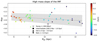 |
Fig. 4 High-mass slope, αIMF, of the IMF versus galactocentric radius, Rgc, for each open cluster. The clusters are coloured by their metallicity [Fe/H] and categorised into four age groups. Error bars are the upper and lower bounds of the inferred parameter from the MCMC algorithm. The dashed line is the mean trend of the whole sample, and the shaded region denotes one σ from this trend. The αIMF trend is |

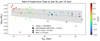 |
Fig. 5 Same as Fig. 4 but for the rate of SNIa (NIa). The NIa trend is |

4.2 Rate of SN la
The number of SN Ia per M⊙ per 15 Gyr(NIa) closely follows the shape of the metallicity gradient traced by the open clusters, as can be seen in Fig. 2. A decreasing rate of SN Ia in the inner Galaxy (6.0 ≤ Rgc ≤ 7.0 kpc) is followed by a plateau in the outer Galaxy (Fig. 5). The metallicity gradient that is seen today in the Milky Way correlates with the number of SN Ia occurring during the formation of the Galaxy. Overall,
we find a linear trend with respect to the galactocentric radius of  SN Ia events per M⊙ per 15 Gyr per kpc.
When compared to the prior distribution of log10(NIa)= −2.75 ± 0.3, the results are relatively close to this value, with a slight bias towards a lower SN Ia rate. The young clusters at solar Rgc have a large spread in their results, which appear to be in all of the free parameters for the clusters in the solar neighbourhood.
4.3 Star formation rate
Figure 6 shows that the S F Rpeak parameter is the least certain in our model, with the largest errors across the free parameters. This is due to the spread in the MCMC chain for this parameter, described in Appendix A. However, we find trends that are similar to that of the other parameters. Firstly, there is a slight overall positive slope with the inner Galaxy near log10(S F Rpeak) ≈ 0.55, which is near the mean of our prior distribution of 3.5 ± 1.5 Gyr(log10(3.5) ≈ 0.55), increasing to S F Rpeak ≈ 5 Gyr(log10(S F Rpeak) ≈ 0.7) in the outer Galaxy. This overall linear trend has a global gradient of  Gyr per kpc.
Our S F Rpeak results show a difference between the inner and outer Galaxy, where the inner Galaxy shows a more intense star formation early in the formation, while the outer Galaxy has a more sustained star formation. Which is consistent with the observed metallicity gradient and the rate of SNIa results.
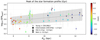 |
Fig. 6 Same as Fig. 4 but for the star formation rate peak S F Rpeak parameter. The S F Rpeak trend is |

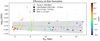 |
Fig. 7 Same as Fig. 4 but for the star formation efficiency (SFE) parameter. The SFE trend is |

4.4 Star formation efficiency
The star formation efficiency (SFE) results shown in Fig. 7 display inefficient star formation across the Milky Way, with the majority of the clusters around log10(S F E) ≈−0.85. The outliers have an increased SFE; however, the uncertainties are large compared with the other results. All the results, bar a few outliers in the inner Galaxy, are more inefficient than our prior of log10(S F E)=−0.3. We find SFE has a linear gradient of  per kpc.
Chempy defines the SFE as SFE = (sum of SFR)/(sum of ISM Gas), which directly relates how much mass is contained within stars to how much mass is in the ISM. If the SFE is low, then the star formation is inefficient, meaning the ISM contains much more gas than what has been formed into stars. Conversely, if the SFE is high, it implies efficient star formation, meaning the star formation has used more of the available nearby ISM gas.
Our low SFE results across the entire Galaxy may be an effect of using open clusters as our point of reference. Open clusters are formed in star-forming regions, and these regions naturally have a lot of gas and dust in them to form the observed open cluster members. Thus, we may expect to see low SFE so that our model properly emulates the star-forming regions where open clusters were born.
4.5 Outliers
The shaded regions in Figs. 4, 5, 6, and 7 denote one σ from the mean trend. Any clusters outside of these regions are classified as ‘outliers’. While 1−σ is not significant, we used this to investigate if there is real physical diversity or just limits of what the modelling delivers.
IMF outliers
In the outer Galaxy, there is a group of four open clusters with a flattening IMF over 1 kpc(10.5 ≤ Rgc ≤ 11.5 kpc) from approximately −2.4 to −2.0. This group appears to lead to another open cluster at ∼ 13 kpc with a shallow IMF. These five clusters are Haffner 10, NGC2425, Berkeley 32, Berkeley 39, and ESO 92-05. Clusters Haffner 10, NGC2425, and Berkeley 32 are kinematically hot with a velocity of Vtot>70 km s−1, indicating that they may be part of the galactic thick disc. Berkeley 39 is a massive open cluster, but it does not show any obvious peculiarities to suggest it being an outlier (Bragaglia et al. 2022). ESO 92-05, however, is far from the Galactic plane at |Z|= 1.6 kpc. Ortolani et al. (2008) suggests ESO 92-05 could be formed as a result of the accretion with a dwarf galaxy in which the activity may have triggered additional localised star formation from the resultant mixed gas cloud. Thus, ESO 92-05 is likely not formed from the same thick and thin discs as the other Milky Way clusters.
Two additional outliers have a steep IMF: γ Velorum, a young 20 Myr near solar radius, and Berkeley 22, an old 2.4 Gyr cluster Rgc=14.3 kpc. Jeffries et al. (2014) notes that γ Velorum has two stellar populations within its cluster members, namely, a dense inner cluster population and a low-mass dispersed population that surrounds the inner cluster. This could be a reason for γ Velorum being an outlier in our results. Berkeley 22 has also been suggested to be a result of an accretion event by Frinchaboy et al. (2004); however, Di Fabrizio et al. (2005) reviewed Berkeley 22 and found a lack of evidence for Berkeley 22 being abnormal.
SNIa outliers
In the outer Galaxy clusters, we found three outlier clusters with a lower SNIa rate than the trend: NGC2243, ESO 92-05, and Berkeley 22. ESO 92-05 and Berkeley 22 have been discussed already as potentially being a result of a galactic accretion event. NGC2243 is a metal-poor, [Fe/H]=−0.45 ± 0.05, cluster far from the Galactic plane, |Z|=1.15 kpc, with a high velocity, Vtot ≈ 80 km s−1, making it kinematically similar to the thick disc population. NGC2243 has also been widely studied for the so-called ‘lithium dip’ in open clusters (François et al. 2014; Anthony-Twarog et al. 2021).
In the inner Galaxy, we found one outlier with the lowest SNIa rate,  : Berkeley 44. It is a metalrich, [Fe/H]=0.22 ± 0.09, inner Galaxy cluster. Carraro et al. (2006) investigated whether Berkeley 44 can be attributed to an accretion event or whether this cluster could be explained by the thick disc and halo population. Their results are not conclusive, but they still provided us with the information that Berkeley 44 is likely not a regular thin disc open cluster.
SFR outliers
We found a sharp increase and deviation from the trend in the region 10.5<Rgc<11.5 kpc, similar to the αIMF parameter. The outliers in this region are NGC2243, NGC2420, NGC2425, Berkeley 32, Trumpler 5, and Berkeley 39. NGC2243, Berkeley 32, and Berkeley 39 have been identified as outliers in the other parameters already.
NGC2420 and NGC2425 are two old clusters with |Z|<1 kpc and are kinematically hot, with Vtot > 70 km s−1. Donati et al. (2015) investigated Trumpler 5 and found it has no peculiarities in stellar parameters. However, the chemical abundances of Mg, Nd, and Al match the ratios similar to the thick disc, while other elements such as Ni, Ca, Y, and Na are more similar to that of the thin disc. This makes Trumper 5 a chemical anomaly.
Three clusters have a low S F Rpeak value relative to the overall population: Berkeley 44, NGC6281, and Berkeley 22. Berkeley 44 and 22 have both been discussed as clusters potentially resulting from an accretion event. NGC6281 is an intermediate-aged (200 Myr) cluster near the solar galactocentric radius with solar metallicity. The location and velocity of NGC6281 make it likely to be a thin disc cluster.
SFE outliers
There are two metal-rich inner Galaxy outliers: Berkeley 44, which has been discussed already, and NGC6802, a 660 Myr slightly metal-enriched cluster, [Fe/H]=0.14 ± 0.04, which has a high Vtot ≈ 75 km s−1. NGC6802 is used as a target for calibrating abundances in the Gaia-ESO open cluster survey, and it shows no additional peculiarities (Tang et al. 2017).
Near the solar galactocentric radius, there are two outliers with efficient star formation: NGC6281 and NGC3532. NGC6281 has been mentioned before, showing thin-disc-like properties and no other peculiarities. Fritzewski et al. (2021) and references within that work establish NGC3532 as a benchmark open cluster, indicating that this cluster is not indicative of being an outlier in the results.
In the outer Galaxy, Rgc>10 kpc, we observed what appears to be two sequences of results. The more efficient population sits at the upper edge of the shaded region and consists of open clusters: NGC2243, Berkeley 36, NGC2141, Berkeley 22, Berkeley 21, and Berkeley 31. NGC2243 and Berkeley 22 have been found as outliers already.
Berkeley 36, 21, and 31 are all slightly metal poor [Fe/H] ∼ −0.2, have a low velocity, and are situated close to the Galactic plane and thus likely formed from the thin disc. However, Gozha et al. (2012) found Berkeley 21 and 31 to have highly eccentric high orbits, suggesting these open clusters may be formed from the thick-disc or may have an origin not related to the Milky Way.
5 General discussion
Our results in Figs. 4, 5, 6, and 7 are consistent with recent studies using field stars (Hayden et al. 2015; Buck 2020) and open clusters (Spina et al. 2022). These studies suggest that the inner and outer galactic regions may have different evolutionary histories.
The results in the outer Galaxy contain most of the outliers with different evolutionary histories. Many of these outliers have supporting evidence of being a result of accretion events, which triggered star formation in externally contaminated clouds of gas.
These outliers affect our interpretation of trends against Rgc, which is why we reviewed them individually in Sect. 4.5. They nonetheless present an interesting sample of clusters that could hold valuable insights into the Galaxy’s evolutionary history, but this is left for a future study to investigate further.
As SN Ia are responsible for a large fraction of iron, we expected to see a trend in the SN Ia that matches the metallicity gradient traced by the open clusters of the Galaxy (Magrini et al. 2009, 2023; Palla et al. 2024). Our results appear to match the observed metallicity gradient with respect to Rgc for both the star formation rate (an anti-correlate) and the SN Ia rate (a correlate).
All four of our free parameters show a variation in the solar neighbourhood. The group of open clusters in this region appear to be shifted away from the overall trend. This observation may suggest a unique local environment, potentially influenced by intrinsic dispersions in key physics, such as the process of star formation, mixing efficiency, or chemical enrichment.
One reason may be that near Rgc ≈ 8 kpc is a transition region where the metallicity gradient in open clusters forms a ‘knee’ and begins to plateau for the outer Galaxy (Bensby et al. 2011; Spina et al. 2022). This transition region is a region of mixing between thin and thick discs (Hayden et al. 2015; Haywood et al. 2024), where the solar neighbourhood shows two distinct populations in their [α/Fe] abundances. However, this variance in results should also be apparent in the inner Galaxy, where both the thick and thin discs are mixing, which our results do not show.
The disc structure and dust in the Galactic plane obscure young open clusters in the inner and outer regions, complicating the ability to correlate stellar populations across these different regions. The solar neighbourhood, where both young and old populations coexist, allows for a more integrated view across the stellar ages.
When averaged over age, the metallicity and [α/Fe] variance are consistent with the global trends observed in Figs. 4–7. This reinforces that despite local complexities and small-scale variations, the large-scale trends observed agree with the broader Galactic evolution.
From inspecting the four model parameters for inter-dependencies, we found that the results indicate the slope of the IMF, αIMF, is positively correlated with the rate of SNIa, NIa, and weakly correlated with the rate of star formation, S F Rpeak. The correlation with NIa may be due to the formalism of SN Ia DTD, which is used to calculate the rate of SN Ia that depends on the IMF (Maoz et al. 2010; Matteucci 2021). The correlation of αIMF with S F Rpeak indicates two relations. First, a formation history with sustained star formation has a top-heavy IMF, which forms more high-mass stars. Secondly, an intense star formation history over a short period may be a formation history that favours a bottom-heavy IMF, thus producing less massive stars. The NIa is also positively correlated with S F Rpeak, which may be due to a higher star formation history having a higher probability of producing progenitor systems that lead to SN Ia explosions.
We also find that the SFE is anti-correlated with all other parameters. This is due to the SFE parameter directly controlling how much gas is available in the system for star formation, whereas the αIMF, NIa, and S F Rpeak control the production of heavy elements. If SFE is low, there is a large amount of unused gas diluting the ISM and reducing star formation, thus the other parameters need to compensate to match the observed abundances. Similar anti-correlations are found in the Chempy paper (Rybizki et al. 2017, Sect. 5.2.1, Fig. 12), and the anti-correlations have been found by Blancato et al. (2019) and Horta et al. (2022) using field stars.
6 Conclusions
In this paper, we have explored how the evolutionary parameters of the Galaxy change between the inner and outer Galaxy. We selected stars from the open cluster program in the Gaia-ESO spectroscopic survey (Randich et al. 2022; Bragaglia et al. 2022; Gilmore et al. 2022). We removed the abundance measurements with large uncertainties or a low signal-to-noise to ensure a highquality sample of measurements. We selected only those stars with a high membership probability and that had a nearly complete set of abundances in the elements C, N, O, Mg, Si, Ca, Ti, Fe, Mn, Zn, Y, and Ba. Our selection criteria reduced the Gaia-ESO open cluster sample of 32 440 stars to 3379−10.42% of the observed stars, where 71% of the stars were not cluster members. This reduced the total 80 open clusters to 48 usable clusters. We used the one-zone chemical evolution code, Chempy, to find the best-fit evolutionary parameters that predict the measured abundances of our selected open clusters.
Our results reveal that the inner and outer regions of the Galaxy have different formation and evolutionary histories. This difference may be explained by a mixing of the thick disc with the thin disc in the inner Galaxy, contaminating the chemical composition of the star-forming region in which the open cluster formed. The solar neighbourhood appears as a unique transitional region where mixing between galactic discs (thin and thick discs, and the inner and outer Galaxy) occurs, making the solar Rgc an intriguing region for testing the model assumptions.
The inner Galaxy in our model agrees with the formation as proposed in the literature (values can be found in Table 3) except for the star formation efficiency, which may be a bias of using open clusters. The outer Galaxy in our model deviates from the older literature, suggesting that the chemical evolution in this region may be altered by external events such as accretion from satellite dwarf galaxies.
Future developments will consider other theoretical models for the galactic evolutionary parameters, for example, the impact of a time-varying initial mass function on the GCE code’s predictive accuracy. Additionally, the other parameters (outflow fraction, coronal reservoir size, and delay-time distribution delay parameter) provided by Chempy should be included to investigate their effects and inter-parameter correlations. Furthermore, utilising data from additional spectroscopic open cluster surveys and a further complete set of abundance measurements from another survey will provide more comprehensive observational constraints for the model.
Acknowledgements
We thank Dr. Sven Buder for his insightful feedback about the project and results. We are also grateful to Dr. Chiaki Kobayashi for her valuable discussions on yield tables, which greatly enhanced our understanding of the numerical simulations. Additionally, we acknowledge the Gaia-ESO survey for providing the comprehensive dataset of open clusters that was essential for our analysis. TB was funded by project grant no. 2024-04990 from the Swedish Research Council. E.S., A.D., and G.T. acknowledge funding from the Research Council of Lithuania (LMTLT, grant no. P-MIP-23-24). Based on data products from observations made with ESO Telescopes at the La Silla Paranal Observatory under programmes ID 188.B-3002, 193-B-0936, and 197.B-1074. These data products have been processed by the Cambridge Astronomy Survey Unit (CASU) at the Institute of Astronomy, University of Cambridge, and by the FLAMES/UVES reduction team at INAFOsservatorio Astrofisico di Arcetri. Public access to the data products is via the ESO Archive, and the Gaia-ESO survey data archive, prepared and hosted by the Wide Field Astronomy Unit, Institute for Astronomy, University of Edinburgh, which is funded by the UK Science and Technology Facilities Council. This research has been partially funded by MICIU/AEI/10.13039/501100011033/ through grant PID2023-146210NB-I00.
References
- Andrews, B. H., Weinberg, D. H., Schönrich, R., & Johnson, J. A., 2017, ApJ, 835, 224 [NASA ADS] [CrossRef] [Google Scholar]
- Anthony-Twarog, B. J., Deliyannis, C. P., & Twarog, B. A., 2021, AJ, 161, 159 [Google Scholar]
- Battistini, C., & Bensby, T., 2016, A&A, 586, A49 [NASA ADS] [CrossRef] [EDP Sciences] [Google Scholar]
- Bensby, T., Feltzing, S., Lundström, I., & Ilyin, I., 2005, A&A, 433, 185 [NASA ADS] [CrossRef] [EDP Sciences] [Google Scholar]
- Bensby, T., Alves-Brito, A., Oey, M. S., Yong, D., & Meléndez, J., 2011, ApJ, 735, L46 [NASA ADS] [CrossRef] [Google Scholar]
- Blancato, K., Ness, M., Johnston, K. V., Rybizki, J., & Bedell, M., 2019, ApJ, 883, 34 [NASA ADS] [CrossRef] [Google Scholar]
- Blomme, R., Daflon, S., Gebran, M., et al. 2022, A&A, 661, A120 [NASA ADS] [CrossRef] [EDP Sciences] [Google Scholar]
- Bovy, J., 2016, ApJ, 817, 49 [NASA ADS] [CrossRef] [Google Scholar]
- Bragaglia, A., Sestito, P., Villanova, S., et al. 2008, A&A, 480, 79 [NASA ADS] [CrossRef] [EDP Sciences] [Google Scholar]
- Bragaglia, A., Alfaro, E. J., Flaccomio, E., et al. 2022, A&A, 659, A200 [NASA ADS] [CrossRef] [EDP Sciences] [Google Scholar]
- Buck, T., 2020, MNRAS, 491, 5435 [NASA ADS] [CrossRef] [Google Scholar]
- Carraro, G., Subramaniam, A., & Janes, K. A., 2006, MNRAS, 371, 1301 [NASA ADS] [CrossRef] [Google Scholar]
- Chen, L., Hou, J. L., & Wang, J. J., 2003, AJ, 125, 1397 [NASA ADS] [CrossRef] [Google Scholar]
- Chiappini, C., Matteucci, F., & Gratton, R., 1997, ApJ, 477, 765 [Google Scholar]
- Côté, B., & Ritter, C., 2018, Astrophysics Source Code Library [record ascl:1806.018] [Google Scholar]
- Côté, B., O’Shea, B. W., Ritter, C., Herwig, F., & Venn, K. A., 2017, ApJ, 835, 128 [Google Scholar]
- Di Fabrizio, L., Bragaglia, A., Tosi, M., & Marconi, G., 2005, MNRAS, 359, 966 [Google Scholar]
- Donati, P., Cocozza, G., Bragaglia, A., et al. 2015, MNRAS, 446, 1411 [NASA ADS] [CrossRef] [Google Scholar]
- Elmegreen, B. G., & Efremov, Y. N., 1997, ApJ, 480, 235 [Google Scholar]
- François, P., Pasquini, L., Biazzo, K., Bonifacio, P., & Palsa, R., 2014, Conference: Origin of Matter and Evolution of Galaxies 2013, 1594, 99 [Google Scholar]
- Frinchaboy, P. M., Majewski, S. R., Crane, J. D., et al. 2004, ApJ, 602, L21 [Google Scholar]
- Fritzewski, D. J., Barnes, S. A., James, D. J., Järvinen, S. P., & Strassmeier, K. G., 2021, A&A, 656, A103 [NASA ADS] [CrossRef] [EDP Sciences] [Google Scholar]
- Gilmore, G., Randich, S., Worley, C. C., et al. 2022, A&A, 666, A120 [NASA ADS] [CrossRef] [EDP Sciences] [Google Scholar]
- Gjergo, E., Sorokin, A. G., Ruth, A., et al. 2023, ApJS, 264, 44 [Google Scholar]
- Goodman, J., & Weare, J., 2010, Commun. Appl. Math. Computat. Sci., 5, 65 [Google Scholar]
- Gozha, M. L., Koval’, V. V., & Marsakov, V. A., 2012, Astron. Lett., 38, 519 [Google Scholar]
- Hayden, M. R., Bovy, J., Holtzman, J. A., et al. 2015, ApJ, 808, 132 [Google Scholar]
- Haywood, M., Khoperskov, S., Cerqui, V., et al. 2024, A&A, 690, A147 [NASA ADS] [CrossRef] [EDP Sciences] [Google Scholar]
- Holmberg, J., Nordström, B., & Andersen, J., 2007, A&A, 475, 519 [CrossRef] [EDP Sciences] [Google Scholar]
- Horta, D., Ness, M. K., Rybizki, J., Schiavon, R. P., & Buder, S., 2022, MNRAS, 513, 5477 [NASA ADS] [CrossRef] [Google Scholar]
- Hourihane, A., François, P., Worley, C. C., et al. 2023, A&A, 676, A129 [NASA ADS] [CrossRef] [EDP Sciences] [Google Scholar]
- Jackson, R. J., Jeffries, R. D., Wright, N. J., et al. 2021, MNRAS, 509, 1664 [NASA ADS] [CrossRef] [Google Scholar]
- Jeffries, R. D., Jackson, R. J., Cottaar, M., et al. 2014, A&A, 563, A94 [NASA ADS] [CrossRef] [EDP Sciences] [Google Scholar]
- Johnson, J. W., & Weinberg, D. H., 2020, MNRAS, 498, 1364 [CrossRef] [Google Scholar]
- Joshi, G. C., 2016, Open Star Cluster: Formation, Parameters, Membership and Importance [Google Scholar]
- Karakas, A. I., 2010, MNRAS, 403, 1413 [NASA ADS] [CrossRef] [Google Scholar]
- Karakas, A. I., 2016, Mem. Soc. Astron. Ital., 87, 229 [Google Scholar]
- Karakas, A. I., & Lugaro, M., 2016, ApJ, 825, 26 [NASA ADS] [CrossRef] [Google Scholar]
- Karakas, A. I., Lugaro, M., & Gallino, R., 2007, Conference: Why Galaxies Care About AGB Stars: Their Importance as Actors and Probes, 378, 37 [Google Scholar]
- Kharchenko, N. V., Piskunov, A. E., Röser, S., Schilbach, E., & Scholz, R. D., 2005, A&A, 438, 1163 [NASA ADS] [CrossRef] [EDP Sciences] [Google Scholar]
- Kobayashi, C., & Nakasato, N., 2011, ApJ, 729, 16 [NASA ADS] [CrossRef] [Google Scholar]
- Kobayashi, C., & Taylor, P., 2023, Chemo-Dynamical Evolution of Galaxies [Google Scholar]
- Kobayashi, C., Umeda, H., Nomoto, K., Tominaga, N., & Ohkubo, T., 2006, ApJ, 653, 1145 [NASA ADS] [CrossRef] [Google Scholar]
- Kobayashi, C., Karakas, A. I., & Lugaro, M., 2020, ApJ, 900, 179 [Google Scholar]
- Krause, M. G. H., Offner, S. S. R., Charbonnel, C., et al. 2020, Space Sci. Rev., 216, 64 [CrossRef] [Google Scholar]
- Kroupa, P., & Boily, C. M., 2002, MNRAS, 336, 1188 [Google Scholar]
- Kroupa, P., Tout, C. A., & Gilmore, G., 1993, MNRAS, 262, 545 [NASA ADS] [CrossRef] [Google Scholar]
- Kroupa, P., Weidner, C., Pflamm-Altenburg, J., et al. 2013, Planets, Stars and Stellar Systems: Galactic Structure and Stellar Populations, 5, The Stellar and Sub-Stellar Initial Mass Function of Simple and Composite Populations (Dordrecht: Springer), 115 [Google Scholar]
- Lada, C. J., & Lada, E. A., 2003, ARA&A, 41, 57 [Google Scholar]
- Liang, J., Gjergo, E., & Fan, X., 2023, MNRAS, stad1013 [Google Scholar]
- Magrini, L., & Randich, S., 2014, EAS Publications Series, 67, 115 [CrossRef] [EDP Sciences] [Google Scholar]
- Magrini, L., Sestito, P., Randich, S., & Galli, D., 2009, A&A, 494, 95 [NASA ADS] [CrossRef] [EDP Sciences] [Google Scholar]
- Magrini, L., Viscasillas Vázquez, C., Spina, L., et al. 2023, A&A, 669, A119 [NASA ADS] [CrossRef] [EDP Sciences] [Google Scholar]
- Maoz, D., & Mannucci, F., 2012, PASA, 29, 447 [NASA ADS] [CrossRef] [Google Scholar]
- Maoz, D., Sharon, K., & Gal-Yam, A., 2010, ApJ, 722, 1879 [Google Scholar]
- Martin, N. F., Ibata, R. A., Bellazzini, M., et al. 2004, MNRAS, 348, 12 [Google Scholar]
- Matteucci, F., 2001, Astrophys. Space Sci. Libr., 253 [Google Scholar]
- Matteucci, F., 2021, A&A Rev., 29, 5 [NASA ADS] [CrossRef] [Google Scholar]
- Minchev, I., Chiappini, C., & Martig, M., 2013, A&A, 558, A9 [CrossRef] [EDP Sciences] [Google Scholar]
- Nomoto, K., Kobayashi, C., & Tominaga, N., 2013, ARA&A, 51, 457 [CrossRef] [Google Scholar]
- Ortolani, S., Bica, E., & Barbuy, B., 2008, MNRAS, 388, 723 [NASA ADS] [CrossRef] [Google Scholar]
- Pagel, B. E. J., & Tautvaisiene, G., 1995, MNRAS, 276, 505 [NASA ADS] [CrossRef] [Google Scholar]
- Pagel, B. E. J., & Tautvaisiene, G., 1997, MNRAS, 288, 108 [Google Scholar]
- Palla, M., Magrini, L., Spitoni, E., et al. 2024, A&A, 690, A334 [NASA ADS] [CrossRef] [EDP Sciences] [Google Scholar]
- Pancino, E., Lardo, C., Altavilla, G., et al. 2017, A&A, 598, A5 [NASA ADS] [CrossRef] [EDP Sciences] [Google Scholar]
- Pasquini, L., Avila, G., Blecha, A., et al. 2002, The Messenger, 110, 1 [Google Scholar]
- Philcox, O., Rybizki, J., & Gutcke, T. A., 2018, ApJ, 861, 40 [Google Scholar]
- Piecka, M., & Paunzen, E., 2021, Structure of Open Clusters – Gaia DR2 and Its Limitations [Google Scholar]
- Poovelil, V. J., Zasowski, G., Hasselquist, S., et al. 2020, ApJ, 903, 55 [NASA ADS] [CrossRef] [Google Scholar]
- Prantzos, N., Abia, C., Chen, T., et al. 2023, MNRAS, 523, 2126 [NASA ADS] [CrossRef] [Google Scholar]
- Randich, S., Gilmore, G., Magrini, L., et al. 2022, A&A, 666, A121 [NASA ADS] [CrossRef] [EDP Sciences] [Google Scholar]
- Reddy, A. B. S., Lambert, D. L., & Giridhar, S., 2016, MNRAS, 463, 4366 [NASA ADS] [CrossRef] [Google Scholar]
- Reddy, A. B. S., Giridhar, S., & Lambert, D. L., 2020, J. Astrophys. Astron., 41, 38 [Google Scholar]
- Ritter, C., Herwig, F., Jones, S., et al. 2018, MNRAS, 480, 538 [NASA ADS] [CrossRef] [Google Scholar]
- Roškar, R., Debattista, V. P., Quinn, T. R., Stinson, G. S., & Wadsley, J., 2008, ApJ, 684, L79 [Google Scholar]
- Rybizki, J., Just, A., & Rix, H.-W., 2017, A&A, 605, A59 [NASA ADS] [CrossRef] [EDP Sciences] [Google Scholar]
- Seitenzahl, I. R., Ciaraldi-Schoolmann, F., Röpke, F. K., et al. 2013, MNRAS, 429, 1156 [NASA ADS] [CrossRef] [Google Scholar]
- Sestito, P., Bragaglia, A., Randich, S., et al. 2006, A&A, 458, 121 [CrossRef] [EDP Sciences] [Google Scholar]
- Sestito, P., Bragaglia, A., Randich, S., et al. 2008, A&A, 488, 943 [NASA ADS] [CrossRef] [EDP Sciences] [Google Scholar]
- Smiljanic, R., Korn, A. J., Bergemann, M., et al. 2014, A&A, 570, A122 [NASA ADS] [CrossRef] [EDP Sciences] [Google Scholar]
- Spina, L., Magrini, L., & Cunha, K., 2022, Universe, 8, 87 [NASA ADS] [CrossRef] [Google Scholar]
- Spina, L., Magrini, L., Sacco, G. G., et al. 2022, A&A, 668, A16 [NASA ADS] [CrossRef] [EDP Sciences] [Google Scholar]
- Spitoni, E., Cescutti, G., Minchev, I., et al. 2019, A&A, 628, A38 [NASA ADS] [CrossRef] [EDP Sciences] [Google Scholar]
- Stanghellini, L., & Haywood, M., 2010, ApJ, 714, 1096 [NASA ADS] [CrossRef] [Google Scholar]
- Steinmetz, M., 2012, Astron. Nachr., 333, 523 [NASA ADS] [CrossRef] [Google Scholar]
- Strobel, A., 1991, Astron. Nachr., 312, 177 [NASA ADS] [CrossRef] [Google Scholar]
- Talbot, Jr., R. J., & Arnett, W. D. 1971, ApJ, 170, 409 [NASA ADS] [CrossRef] [Google Scholar]
- Tang, B., Geisler, D., Friel, E., et al. 2017, A&A, 601, A56 [NASA ADS] [CrossRef] [EDP Sciences] [Google Scholar]
- Timmes, F. X., Woosley, S. E., & Weaver, T. A., 1995, ApJS, 98, 617 [NASA ADS] [CrossRef] [Google Scholar]
- Ting, Y.-S., & Weinberg, D. H., 2022, ApJ, 927, 209 [NASA ADS] [CrossRef] [Google Scholar]
- Tinsley, B. M., 1980, Fundam. Cosmic Phys., 5, 287 [NASA ADS] [Google Scholar]
- Tinsley, B. M., & Larson, R. B., 1978, ApJ, 221, 554 [Google Scholar]
- Worley, C. C., Smiljanic, R., Magrini, L., et al. 2024, The Gaia-ESO Survey: The DR5 Analysis of the Medium-Resolution GIRAFFE and High-Resolution UVES Spectra of FGK-type Stars [Google Scholar]
- Yan, Z., Jerabkova, T., & Kroupa, P., 2017, A&A, 607, A126 [NASA ADS] [CrossRef] [EDP Sciences] [Google Scholar]
Appendix A MCMC convergence
We tested the model accuracy by selecting three open clusters that cover a wide range of the dataset: IC4665, NGC6005, and NGC2243. IC4665 is a young cluster at ∼ 33 Myr with near solar metallicity [Fe/H]=0.01 ± 0.05 and located near the Sun at Rgc=8.0 kpc. NGC6005 is an old open cluster at ∼ 1.26 Gyr that is metal-rich [Fe/H]=0.22 ± 0.03 in the inner Galaxy Rgc=6.5 kpc. NGC2243 is an old relic open cluster at ∼ 4.3 Gyr that is metal-poor [Fe/H]=−0.45 ± 0.05 just outside the solar radius Rgc=10.6 kpc.
We ran MCMC for our four dimensions with Nwalkers=20 walkers for a maximum of 1000 iterations, giving a maximum of 20 000 samples. It is expected that the final portion of the MCMC chain has converged to a particular value. This converged section of the chain is used to calculate the best-fit value by taking the median of this section. We need to evaluate whether the simulation setup and choice of free parameters allow the MCMC chain to converge.
We used the autocorrelation time τ, Eq. (1), to determine if the posterior has converged. For every N=100 iterations, we evaluate if the length of the chain is greater than L=100 times the autocorrelation time. We also check if the change in the autocorrelation time Δ τ between checks is less than d=5%. Both these checks provide a strong indication that the chain has converged and is unlikely to change further.
In Fig. A.1 we plot the MCMC chains for open clusters IC4665, NGC6005, and NGC2243. In each of the sub-figures, the first row shows the entire raw chain, and the second row shows the converged part of the chain. Columns from left to right are the posterior, parameter values for the IMF (αIMF), rate of SNIa (log10(NIa)), star formation efficiency (log10(S F E)), and the peak and shape of star formation (log10(S F Rpeak)). The cyan line shows the prior value from Table 3 and the red line shows the best-fit value.
IC4665 and NGC6005 stopped at ∼ 5000 samples (∼ 250 iterations). NGC2243 stopped at ∼ 3700 samples (∼ 185 iterations). This is a quarter of the maximum iterations allowed; however, in testing a full 1000 iterations (no early termination by autocorrelation) we found no additional variance in the chains and the results remained the same.
The best-fit value is taken as the median of the converged part encompassing ∼ 2000 samples. The free parameters αIMF and NIa show strong convergence in all three clusters. Star formation efficiency converges strongly in IC4665 and NGC6005, but shows some uncertainty in NGC2243. S F Rpeak shows as the most uncertain parameter in our test clusters. The model as a whole has converged and the uncertainty in those individual parameters will manifest as large upper and lower uncertainties on the best-fit value.
Appendix B Model accuracy
Using the same test clusters defined in Appendix A, we complete the MCMC inference with two yield sets to test the sensitivity to assumptions and input variables by finding the best-fit parameters in each case. The “default” yield tables are those of our fiducial simulation: Nomoto et al. (2013) for SN II, Seitenzahl et al. (2013) for SN Ia, and Karakas (2016) for AGB nucleosynthesis. The “alternative” yield set changes only the SN II yield to the yields provided by the Nugrid collaboration (Ritter et al. 2018).
Figure B.1 plots the resulting predictions for both the default and alternative yield sets. Across all the elements, the default yield selection has better predictions compared to the alternative yield set. This shows that the selection of yields is an important hyperparameter for numerical simulation models (Karakas 2016; Philcox et al. 2018; Kobayashi & Taylor 2023; Liang et al. 2023).
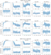 |
Fig. A.1 Markov chain Monte Carlo chains for open clusters IC4665, NGC6005, and NGC2243. The first row shows the raw chain and the second row shows the converged part of the chain. Plots from left to right are posterior, positions for the IMF αIMF, rate of SNIa log10(NIa), star formation efficiency log10(S F E), and the peak and shape of star formation log10(S F Rpeak). The cyan line shows the prior value and the red line shows the best-fit value. |
The iron-peak elements Fe and Ni are now within ∼ 0.1 dex for the default yields, but Mn is overproduced by ∼ 0.2 dex. The alternative yields for the iron-peak elements are greater than ∼ 0.3 dex from the observed abundances. For the α-elements the default yield set still underproduces Ca and Mg, but they are both within ∼ 0.1 dex. Ti shows as severely underproduced in all three clusters; Ti and nearby elements in atomic number are underproduced in most numerical models (Kobayashi et al. 2006). Ba is overproduced with the AGB yields from Karakas (2016) but is the most accurate of the yield tables we can access.
The results of Fig. B.1 do not match all observations within observed uncertainties for several elements. However, we could still extract useful information from the trends in the free parameters.
The inaccuracies in the abundances are likely due to simplifying assumptions in our chemical evolution model. Chempy is a one-zone chemical evolution model that is inherently inaccurate in modelling complex environments such as the Milky Way. We reduce the impact of the one-zone model by assuming each open cluster is born from a unique molecular cloud within the Milky Way, allowing us to model each open cluster as a single isolated zone that is part of a complex multi-zone system. Chempy also models only three of the important enrichment channels and does not include more complex channels such as neutron star mergers, black hole interactions, fast rotating, and highly magnetic stars. This reduces the accuracy of the model as some chemical elements, such as r-process elements, are not modelled. Additionally, there are uncertainties in the nucleosynthetic yield calculations due to effects such as stellar rotation and black hole formation.
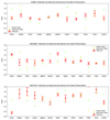 |
Fig. B.1 Model predictions for open clusters IC4665, NGC6005, and NGC2243 with the free parameters set to their best-fit values. Observed abundances in red (cross with error bars denoting abundance uncertainty calculated as per Sect. 2.1) and the prediction from the default and alternative yield sets in orange (▴) and green (▾), respectively. |
Appendix C Chempy likelihood comparison of fewer elements
We select three elements, Mg, Fe, and Ba, to isolate the modelled enrichment channels to a single element each and therefore does not consider elements produced from multiple channels. With only three observational constraints to the model, we may be concerned with the lack of data representing the complex chemical composition of open clusters. The three-element simulation has a much higher likelihood compared to the full-element simulation. This accuracy may be due to a few factors such as overfitting; overfitting is a concern as we have four free parameters to fit three observations.
Conversely, the full-element simulation introduces a lot of variance across the observations. Still, it includes complex chemical compositions which our simple one-zone model and limited enrichment channels may not fully represent. Further increasing the element count worsens this effect. Thus, we find the selection of 12 elements is a balance between these effects.
Table C.1 tabulates each open cluster along with their literature metallicity [Fe/H], galactocentric radius Rgc, age in Myr, and the number of stellar members selected from our data selection. The last four columns show a comparison of the likelihoods of the model for the default yields and the alternative yields for both the three-element model and the full-element model.
Open cluster properties and Chempy log likelihoods}
All Tables
All Figures
|
Fig. 1 Sample selection from the Gaia-ESO DR5 open cluster dataset. The base dataset is shown in grey, and the selected data after processing and cleaning are shown in blue. |
| In the text | |
|
Fig. 2 Final sample of open cluster stars. Left: galactic location of the open clusters, where the dark-green dotted circle and solid circle denote the solar radius and the galactic centre, respectively. The inset shows a closer view of the clusters in the solar neighbourhood. Right: open cluster ages (top), height above the Galactic plane (middle), and metallicity [Fe/H] (bottom), each against galactocentric radius. The colour map of [Fe/H] is the same for all four plots.} |
| In the text | |
|
Fig. 3 Uncertainty distribution of abundance measurements from the GES DR5 open cluster dataset before (grey) and after (blue) the percentile filter was applied. |
| In the text | |
|
Fig. 4 High-mass slope, αIMF, of the IMF versus galactocentric radius, Rgc, for each open cluster. The clusters are coloured by their metallicity [Fe/H] and categorised into four age groups. Error bars are the upper and lower bounds of the inferred parameter from the MCMC algorithm. The dashed line is the mean trend of the whole sample, and the shaded region denotes one σ from this trend. The αIMF trend is |
| In the text | |
|
Fig. 5 Same as Fig. 4 but for the rate of SNIa (NIa). The NIa trend is |
| In the text | |
|
Fig. 6 Same as Fig. 4 but for the star formation rate peak S F Rpeak parameter. The S F Rpeak trend is |
| In the text | |
|
Fig. 7 Same as Fig. 4 but for the star formation efficiency (SFE) parameter. The SFE trend is |
| In the text | |
|
Fig. A.1 Markov chain Monte Carlo chains for open clusters IC4665, NGC6005, and NGC2243. The first row shows the raw chain and the second row shows the converged part of the chain. Plots from left to right are posterior, positions for the IMF αIMF, rate of SNIa log10(NIa), star formation efficiency log10(S F E), and the peak and shape of star formation log10(S F Rpeak). The cyan line shows the prior value and the red line shows the best-fit value. |
| In the text | |
|
Fig. B.1 Model predictions for open clusters IC4665, NGC6005, and NGC2243 with the free parameters set to their best-fit values. Observed abundances in red (cross with error bars denoting abundance uncertainty calculated as per Sect. 2.1) and the prediction from the default and alternative yield sets in orange (▴) and green (▾), respectively. |
| In the text | |
Current usage metrics show cumulative count of Article Views (full-text article views including HTML views, PDF and ePub downloads, according to the available data) and Abstracts Views on Vision4Press platform.
Data correspond to usage on the plateform after 2015. The current usage metrics is available 48-96 hours after online publication and is updated daily on week days.
Initial download of the metrics may take a while.