| Issue |
A&A
Volume 705, January 2026
|
|
|---|---|---|
| Article Number | A232 | |
| Number of page(s) | 14 | |
| Section | Numerical methods and codes | |
| DOI | https://doi.org/10.1051/0004-6361/202556424 | |
| Published online | 26 January 2026 | |
The miniJPAS survey quasar selection
V. Combined algorithm
1
Departament de Física, EEBE, Universitat Politècnica de Catalunya,
c/Eduard Maristany 10,
08930
Barcelona,
Spain
2
Institut de Física d’Altes Energies (IFAE), The Barcelona Institute of Science and Technology, Campus UAB,
08193
Bellaterra Barcelona,
Spain
3
Departamento de Física Matemática, Instituto de Física, Universidade de São Paulo,
Rua do Matão 1371,
CEP
05508-090,
São Paulo,
Brazil
4
Instituto de Astrofísica de Andalucía (CSIC),
PO Box 3004,
18080
Granada,
Spain
5
Aix Marseille Univ, CNRS, CNES, LAM,
Marseille,
France
6
Observatório Nacional, Rua General José Cristino,
77, São Cristóvão,
20921-400
Rio de Janeiro,
RJ,
Brazil
7
Donostia International Physics Center (DIPC),
Manuel Lardizabal Ibilbidea, 4,
San Sebastián,
Spain
8
Centro de Estudios de Física del Cosmos de Aragón (CEFCA),
Plaza San Juan, 1,
44001
Teruel,
Spain
9
Unidad Asociada CEFCA-IAA, CEFCA, Unidad Asociada al CSIC por el IAA y el IFCA,
Plaza San Juan 1,
44001
Teruel,
Spain
10
Departamento de Física, Universidade Federal do Espírito Santo,
29075-910
Vitória,
ES,
Brazil
11
INAF – Osservatorio Astronomico di Trieste,
via Tiepolo 11,
34131
Trieste,
Italy
12
IFPU – Institute for Fundamental Physics of the Universe,
via Beirut 2,
34151
Trieste,
Italy
13
Observatori Astronòmic de la Universitat de València, Ed. Instituts d’Investigació,
Parc Científic. C/ Catedrático José Beltrán, n2,
46980
Paterna, Valencia,
Spain
14
Departament d’Astronomia i Astrofísica, Universitat de València,
46100
Burjassot,
Spain
15
Instituto de Astrofísica de Canarias, C/ Vía Láctea, s/n,
38205
La Laguna, Tenerife,
Spain
16
Universidad de La Laguna, Avda Francisco Sánchez,
38206
San Cristóbal de La Laguna, Tenerife,
Spain
17
Departamento de Astronomia, Instituto de Astronomia, Geofísica e Ciências Atmosféricas, Universidade de São Paulo,
São Paulo,
Brazil
18
Instruments4,
4121 Pembury Place,
La Canada Flintridge,
CA
91011,
USA
★ Corresponding author: This email address is being protected from spambots. You need JavaScript enabled to view it.
Received:
15
July
2025
Accepted:
7
November
2025
Abstract
Aims. Quasar catalogues from narrow-band photometric data are used in a variety of applications, including targeting for spectroscopic follow-up, measurements of supermassive black hole masses, or baryon acoustic oscillations. Here, we present the final quasar catalogue, including redshift estimates, from the miniJPAS Data Release constructed using several flavours of machine-learning algorithms.
Methods. In this work, we use a machine learning algorithm to classify quasars, optimally combining the output of eight individual algorithms. We assess the relative importance of the different classifiers. We include results from three different redshift estimators to also provide improved photometric redshifts. We compare our final catalogue against both simulated data and real spectroscopic data. Our main comparison metric is the f1 score, which balances the catalogue purity and completeness.
Results. We evaluate the performance of the combined algorithm using synthetic data. In this scenario, the combined algorithm out-performs the rest of the codes, reaching f1 = 0.88 and f1 = 0.79 for high- and low-z quasars (with z ≥ 2.1 and z < 2.1, respectively) down to magnitude r = 23.6. We further evaluate its performance against real spectroscopic data, finding different performances (some of the codes show a better performance, some a worse one, and the combined algorithm does not outperform the rest). We conclude that our simulated data are not realistic enough and that a new version of the mocks would improve the performance. Our redshift estimates on mocks suggest a typical uncertainty of σNMAD = 0.11, which, according to our results with real data, could be significantly smaller (as low as σNMAD = 0.02). We note that the data sample is still not large enough for a full statistical consideration.
Key words: methods: data analysis / techniques: photometric / quasars: general / cosmology: observations
Independent Researcher
© The Authors 2026
 Open Access article, published by EDP Sciences, under the terms of the Creative Commons Attribution License (https://creativecommons.org/licenses/by/4.0), which permits unrestricted use, distribution, and reproduction in any medium, provided the original work is properly cited.
This article is published in open access under the Subscribe to Open model. This email address is being protected from spambots. You need JavaScript enabled to view it. to support open access publication.
1 Introduction
In astronomy, there is now an ever-increasing number of surveys producing increasingly large amounts of data. For instance, multi-slit and/or multi-fibre spectrographs mounted on large telescopes can now obtain thousands of spectra in a single night. Examples of present and future quasar spectroscopic surveys include the fifth generation of the Sloan Digital Sky Survey (SDSS-V; Kollmeier et al. 2017; Almeida et al. 2023), the Dark Energy Spectroscopic Instrument (DESI; Levi et al. 2013; DESI Collaboration 2016a,b, 2024), the Subaru Prime Focus Spectrograph (PFS, Takada et al. 2014), the Multi-Object Optical and Near-infrared Spectrograph (MOONSM Cirasuolo et al. 2011), the 4 metre Multi-Object Spectroscopic Telescope (4MOST; de Jong 2019), Gaia (Storey-Fisher et al. 2024), and the William Herschel Telescope Enhanced Area Velocity Explorer Collaboration (WEAVE; Dalton et al. 2016).
Targets for these spectroscopic surveys are drawn from even larger photometric surveys. These surveys observe many more objects, but the derived properties, such as object classification and redshifts, are less secure. Examples of present and future photometric surveys include the DESI Legacy Imaging Survey (Dey et al. 2019), the Square Kilometer Array (SKA; Dewdney et al. 2009), the Dark Energy Survey (DES; Dark Energy Survey Collaboration 2016), the Panoramic Survey Telescope and Rapid Response System(Pan-STARRS; Chambers et al. 2016), Euclid (Euclid Collaboration: Mellier et al. 2025), the Large Synoptic Survey Telescope (LSST; Ivezić et al. 2019), and the Javalambre Physics of the Accelerating Universe Astrophysical Survey (J-PAS; Benitez et al. 2014).
Amongst other interesting objects, these surveys compile lists of quasars: distant, very powerful galaxies powered by accretion into supermassive black holes at the centre of their host galaxies. Their (optical) spectra present several broad emission lines and an approximate power-law continuous emission in the UV and optical wavelengths. The quasar spectra as a whole are strikingly self-similar (e.g. Merloni 2016 and references therein) and have been widely studied (e.g. Jensen et al. 2016; Lyke et al. 2020; Wu & Shen 2022; Pérez-Ràfols et al., in prep.).
While quasars themselves are very interesting, they are also often used as background sources to study the intergalactic medium, and through it, cosmology. For example, the Lyman α absorption seen in the spectra of quasars has been widely used to constrain cosmology via baryon acoustic oscillations (see e.g. DESI Collaboration 2025 and references therein). Other uses of the Lyman α absorption include intensity mapping studies (e.g. Ravoux et al. 2020; Kraljic et al. 2022, and references therein). The spectra of quasars also allow us to detect a variety of absorption systems, including Damped Lyman α absorbers, containing most of the neutral hydrogen in the Universe (e.g. Brodzeller et al. 2025 and references therein) and, in general, galaxies in absorption (e.g. Morrison et al. 2024; Pérez-Ràfols et al. 2023b).
Of the many applications, here we are interested in the quasar identification and redshift estimation in photometric surveys. Both machine learning and template fitting have been used in this endeavour (see e.g. Salvato et al. 2018 for a review). When machine learning is used, there exist a large number of approaches to distinguish between galaxies, stars, and quasars (see e.g. Krakowski et al. 2016; Bai et al. 2019; Logan & Fotopoulou 2020; Xiao-Qing & Jin-Meng 2021; He et al. 2021). One of the main differences between the different algorithms is the input parameters that are fed to the machine learning algorithms: fluxes, magnitudes, and so on. More recently, even colours measured in different apertures have been used (Saxena et al. 2024).
Similarly, previous papers in this series have introduced different flavours of machine-learning algorithms to construct a quasar catalogue from the miniJPAS survey (Rodrigues et al. 2023; Martínez-Solaeche et al. 2023; Pérez-Ràfols et al. 2023a). The miniJPAS survey is the first data release from the JPAS Collaboration and shows the results of their pathfinder camera (Bonoli et al. 2021). In these papers, we trained our models and assessed their performance, using dedicated mocks (Queiroz et al. 2023). In this work, we present the final combined quasar catalogue, including the results of all previous papers in the series. Instead, here we use an ensemble of algorithms to classify quasars. Indeed, as inputs for the model, we do not use the observed object properties, but rather the results of previous algorithms.
The novelty of this work resides not only in the combination of different algorithms to build classification confidence but also in a much better assessment of the results. Besides assessing the performance with mocks, we additionally tested our algorithms against real data from the DESI Early Data Release (DESI Collaboration 2024).
This paper is organised as follows. In Section 2, we describe the data used in this work, including the individual algorithms from the previous papers in the series. We then describe the combination procedure in Section 3, and assess its performance against mocks in Section 4. In Section 5, we present our quasar catalogue, and we discuss its performance against real data in Section 6. We finish summarising our conclusions in Section 7. Throughout this work, reported magnitudes refer to the AB magnitude system.
2 Data
2.1 miniJPAS data and mocks
This work is centred on the classification of sources from the miniJPAS data release (Bonoli et al. 2021). This is a photometric survey using 56 filters, of which 54 are narrow-band filters ranging from 3780 Å to 9100 Å, with FWHM ~14 Å and 2 are broader filters extending to the UV and the near-infrared. The SDSS broadband filters u, g, r, and i complement the aforementioned 56 filters to reach a total of 60 filters. miniJPAS was run on the AEGIS field and covers ~1deg2. Bonoli et al. (2021) report a limiting magnitude of r = 23.6, defined as the magnitude at which the catalogue is 99% complete.
Sources were identified using the SEXTRACTOR code (Bertin & Arnouts 1996). There are several catalogues available according to the filter(s) used to identify the sources. Here we used the dual mode, in which objects are identified in both the filter of interest and the reference filter (r band). We refer the reader to Bertin & Arnouts (1996); Bonoli et al. (2021) for more detailed explanations of the software and object detection. We cleaned the initial catalogue1, with 64 293 objects, to exclude flagged objects. These flags indicate problems during field reduction and/or object detection and are described in detail in Bonoli et al. (2021). Our final clean sample contains 46 441 objects. We label this sample as ‘all objects’.
At this point, it is worth noting that high-redshift quasars are typically point-like sources. Thus, we defined our main sample, which we label as ‘point-like’, to include only point-like objects. These were found using the stellarity index constructed from image morphology using extremely randomised trees (ERT), a machine learning algorithm performing star-galaxy classification (which we took as a proxy for point-like source classification) with an area under the curve AUC = 0.986 (see Baqui et al. 2021 for a detailed description). Following Queiroz et al. (2023), Rodrigues et al. (2023), Martínez-Solaeche et al. (2023), and Pérez-Ràfols et al. (2023a), we required objects to be classified as stars (point-like sources) with a probability of at least 0.1, defined in their catalogue as ERT ≥ 0.1. In cases in which the ERT classification failed (identified as ERT=99.0), we instead used the alternative classification using the stellar-galaxy locus (SGLC) classifier (first developed by López-Sanjuan et al. 2019 and then adapted to miniJPAS in Bonoli et al. 2021), which uses the morphological information from the g, r, and i broad-band filters. We required a minimum probability of SGLC ≥ 0.1. 11 419 objects meet this point-like source criterion and constitute our point-like sample.
In addition to miniJPAS data, we also used simulated data (mocks). These mocks were already used in the previous papers in the series to train different algorithms (see Section 2.3). Here, we used them as truth tables to (optimally) combine said algorithms. The mocks were based on SDSS spectra, which were convolved with the J-PAS filters. Noise was also added to match the expected signal-to-noise. We refer the reader to Queiroz et al. (2023) for a detailed description of the mocks and their building procedure, but we note that the mocks were defined to match the properties of the point-like objects in miniJPAS. We have a total of 360 000 objects distributed between the training (100 000), validation (30 000), and test (30 000) sets. These samples contain an equal number of stars, quasars, and galaxies. This is not the expected on-sky distribution of sources, but it is convenient in order to train the algorithms. Thus, in addition to these samples, we had a special 1 deg2 test set built in a similar procedure except that it had the expected relative fraction for each type of object, containing 2191 stars, 6410 galaxies, and 510 quasars. Again, we refer the reader to Queiroz et al. (2023) for details on how this sample was built.
In the previous papers in the series, in which we trained the different classifiers that we used here (see Section 2.3), we restricted the analysis to r-band magnitudes of 17.0 < r ≤ 24.3. Thus, we needed to apply the same cut here, which reduced the number of objects in all our samples. Table 1 summarises the final number of objects in each sample, when including this magnitude cut.
Summary of the samples used in this work.
2.2 DESI data
One of the major drawbacks of our previous papers is that we relied solely on mocks to assess the performance of our classifiers. True, there were SDSS spectra with miniJPAS counterparts, but there were too few of them (272) to extract any statistically meaningful information. Fortunately, the DESI Early Data Release (EDR, DESI Collaboration 2024) is now available to use. We found 3730 objects with miniJPAS counterparts. Of these, the DESI automatic classification pipeline Redrock (Bailey et al., in prep.) found 667 stars, 2900 galaxies, and 163 quasars, of which 53 have redshift z ≥ 2.1 and 110 have z < 2.1. However, according to the DESI visual inspection (VI) programme, performed during the survey validation phase, Redrock sometimes fails in its classification (Alexander et al. 2023; Lan et al. 2023). Because we are using this classification as a truth table, and because of the relatively small sample size, we visually inspected all the spectra and fixed a small number of classifications (see Appendix A). We found 491 stars, 2873 galaxies, and 190 quasars, of which 133 were with z < 2.1 and 57 were with z ≥ 2.1. We label this sample ‘DESI cross-match’.
As we did with our main catalogue, we created a smaller ‘DESI cross-match point-like’ catalogue containing only the point-like objects, defined according to miniJPAS data and using the criteria mentioned in Section 2.1. There are a total of 1171 objects split into 655 stars, 357 galaxies, and 159 quasars, of which 111 have z < 2.1 and 48 have z ≥ 2.1. We note that there is a non-negligible fraction (~18%) of quasars that are classified as extended sources by miniJPAS. Of these, 9 are high-z quasars and 22 are low-z quasars. At low redshifts, we often see the galactic emission, and therefore we expect some of them to be classified as extended sources. However, this should not be the case for high-z objects. The high-z sources mislabelled as extended are at the faint end of our magnitude distribution, and this is likely the reason behind the misclassification.
Finally, a few of the objects lie outside our selected magnitude range (see Section 2.1) and were thus discarded from this analysis. This magnitude cut was applied based on the miniJPAS magnitudes associated with these objects (irrespective of the measured DESI magnitude). The final number of objects in each of the samples is summarised in the first block of Table 1. We give a more detailed comparison between the different samples in Appendix B.
Summary of the previous classifiers included in this work.
2.3 Previous classifiers
Unlike in the other papers in the series, we did not directly use miniJPAS data for the classification, but rather the outputs from other codes. We used the outputs from ten algorithms, of which eight are classification algorithms (one of which also provides redshift estimates), and two do not perform classification but provide only redshift estimates. The classifiers are summarised in Table 2, and we describe them in more detail in the following paragraphs.
The first five algorithms, called CNN1, CNN1NE, CNN2 RF, and LGBM, are defined in Rodrigues et al. (2023). The first three are based on convolutional neural networks (CNNs). CNN1 and CNN1NE use the fluxes as 1D arrays of input parameters to perform the classification. The difference between them is that CNN1 also includes the flux errors, whereas CNN1NE does not. CNN2 also uses the fluxes and their errors, but instead of formatting them as 1D arrays, a 2D matrix representation is built. The other two algorithms, RF and LGBM, use different flavours of decision tree to perform the classification, the random forest, and the light gradient boosting machine, respectively. Details on the implementation and performance of these algorithms are given in Rodrigues et al. (2023). They focus on classification using four categories – star, galaxy, low-z quasar (z < 2.1), and high-z quasar (z ≥ 2.1) – and do not provide redshift estimates. We note that the z = 2.1 pivot was chosen because the Lyman α feature enters the optical range at this redshift. Each of the algorithms outputs four quantities for each analysed object corresponding to the confidence of classification for each class. For example, conf_lqso_CNN1 gives the confidence of objects being low-redshift quasars according to the classification by CNN1. They also output the object’s class by selecting the class with maximal confidence. We do not include these columns in our training set as they only contain redundant information.
The following two algorithms are described in Martínez-Solaeche et al. (2023). They use artificial neural networks to classify the object based on the J-PAS magnitudes (ANN1) or the J-PAS fluxes (ANN2). Hybridisation in the training samples is used to prevent the classifiers from becoming overly confident. The output of these codes is the same as the previous 5, and they do not provide redshift estimates.
The last code that performs classification is SQUEZE. SQUEZE was originally developed to run on spectra (Pérez-Ràfols et al. 2020; Pérez-Ràfols & Pieri 2020) and was later adapted to running on miniJPAS data (Pérez-Ràfols et al. 2023a). Its behaviour differs significantly from the previous codes. First, the code looks for emission peaks in the spectra and assigns a set of possible emission lines to each of them. This generates a list of trial redshifts, ztry. For each of these trial redshifts, a set of metrics are computed around the predicted position of the quasar emission lines, which are then fed to a random forest algorithm that determines which of the trial redshifts corresponds to the true quasar redshifts. For each of the possible classifications (the trial redshifts), SQUEZE provides the confidence of the object being a quasar and a redshift estimate. We refer the reader to Pérez-Ràfols et al. (2020) for a more detailed description of SQUEZE. Normally, for each object, the best classification (the one with the largest confidence) is kept, and the rest are discarded. However, there is information present in the subsequent classifications (for example, if more than one emission line is correctly identified, the subsequent classifications will also have high confidence and a similar redshift estimate). Thus, here we keep the best five classifications, which we label as SQUEZE_0 to SQUEZE_4. Each of the classifications contains two variables: the classification confidence, for example conf_SQUEZE_Q, and the classification redshift, for example z_SQUEZE_0. In addition, we include the final classification of SQUEZE, labelled as class_SQUEZE, in terms of the usual four categories: star, galaxy, low-z quasar, and high-z quasar, based on the confidence and redshift of SQUEZE_0. Note that since SQUEZE only discriminates between quasar and non-quasar, none of the entries are classified as stars or galaxies. For non-quasars, we do not have any classification. We flag this with a −1 value for this variable.
Finally, to complement the redshift estimations from SQUEZE we included photometric redshift estimates from QPz (Queiroz, private communication) and LePhare2 (Arnouts & Ilbert 2011). While LePhare determines redshifts through a traditional template-fitting method, QPz employs a multi-dimensional fit based on the principal component analysis of quasar spectra of Yip et al. (2004). These were run on all objects, assuming they are quasars. The redshift estimation was performed using quasar templates, and the output variables were named zphot_QPz and zphot_LePhare, respectively.
3 Combination procedure
As we have seen in the previous papers of the series, each of the classification algorithms can provide a quasar catalogue on its own. However, these catalogues are not the same but have slight differences. All the classifiers will agree on the ‘easier’ quasars3. Other, less clear objects have different classifications depending on the algorithm used. These differences lie in the different flavours of machine learning algorithms used by the individual classifiers. The question is, then, how to (optimally) combine the results from these algorithms to maximise the purity and completeness of the final quasar catalogue.
Maximising either the purity or the completeness is rather easy. If we wish to maximise completeness, it suffices to compile all the objects that are in any of the individual catalogues. Similarly, to maximise the purity, we can keep all the quasars present in all the catalogues. Finding a good compromise between the two is delicate, and we used a second layer of machine learning to solve this optimisation problem.
The classification was made using a random forest classifier, which combines multiple decision trees (a structure where the algorithm makes predictions by splitting the data set based on constraints imposed in terms of the features). Each tree is built with a subsample of the data, using the bootstrap aggregating (bagging; Breiman 1996) technique. Note that we explored using several other machine-learning algorithms for this classification and found that the random forest classifier has the best performance.
We implemented the model using the scikit-learn PYTHON package (Pedregosa et al. 2011). We included all the features described in Section 2.3 except for those belonging to QPz and LePhare (see Section 4.2). Training was performed using the validation set, and we tested our performance on the test and test 1 deg2 mock samples. This was necessary as we required the results of the individual classifiers (which are trained using the training sample) as inputs for our model.
In addition to the object classification, we trained a random forest regressor, which operates similarly to the random forest classifier but for continuous variables, to refine the redshift estimation of the found quasars. The redshift regressor was trained using only the quasars present in the validation sample and applied only to objects classified as quasars. For objects not classified as quasars, we simply assigned NaN to their redshift estimate. We implemented the model using the xgboost PYTHON library (Chen & Guestrin 2016), which allows us to use custom metrics when training the random forests (see below). We included all the features described in Section 2.3.
The standard implementation of the random forest regressor uses the mean squared error (Breiman 2001). Because the errors are squared, the mean squared error metric is sensitive to outliers and penalises large deviations in the model. This works well when the distribution of errors follows (or is close to) a Gaussian distribution. In our case, the error distribution in the photometric redshifts is inherently non-Gaussian. For instance, for bright objects, the error is dominated by line confusion, making a small set of outcomes more likely to be selected. What is more, beyond a certain threshold in redshift error, we do not care about the error itself, and the estimate is labelled as catastrophic (e.g. Bolzonella et al. 2000).
Indeed, we found that using the standard metric was unsuitable for our regression problem. Instead, we used the normalised median absolute deviation (see Section 4.3) as our training metric. In addition, we noted that for bright objects (with r < 22), the random forest estimates were not as good as the individual estimation by QPz. Therefore, we decided to keep the QPz estimates for these objects and apply our estimator only to fainter objects.
4 Performance of the classifiers
We now assess the performance of the combined algorithm and compare it to the performance of the individual algorithms. We start by assessing the classification performance in Section 4.1 and move to analyse the importance of the different classifiers in Section 4.2. We then discuss the redshift precision in Section 4.3. The results are summarised in Table 3.
4.1 Classification performance
We start by assessing the classification performance. Our main scoring metric for the comparison is the f1 score metric (but we also provide the purity and completeness). This metric is convenient as it combines purity and completeness in a single metric:
![Mathematical equation: $\[f_1=\frac{2 p c}{p+c}.\]$](/articles/aa/full_html/2026/01/aa56424-25/aa56424-25-eq1.png) (1)
(1)
This metric helps us balance having high values of purity and completeness. When any of the two becomes too low, then the overall f1 score drops. We compare the f1 score of the different classifiers as a function of the limiting magnitude, i.e. including all the objects brighter than a given magnitude. This will give us an idea of the faintest magnitude at which we can trust the resulting catalogue.
Figure 1 shows the f1 score, purity, and completeness as a function of limiting magnitude for the quasar classes for the test sample. The two classes are high-z quasars (with z ≥ 2.1) and low-z quasars (with z < 2.1)4. The results from the combined algorithms are shown as a thick black line, and we plot the results from the individual classifiers as thin lines of different colours. As was expected, we see that the combined algorithm outperforms the rest of the algorithms.
We computed the f1 score, purity, and completeness down to magnitudes 24.3 because that is the faintest magnitude in our samples. However, we note that we have very few objects at these very faint magnitudes5, which explains the flatness of the curves at the faint end. For high-z-quasars, and considering magnitudes brighter than r = 23.6 (which is the magnitude corresponding to the magnitude at which the miniJPAS survey is 99% complete as stated in Bonoli et al. 2021), we find an f1 score of 0.88 (corresponding to a purity of 0.91 and a completeness of 0.85) for the combined algorithm, and we need to decrease the magnitude limit to r = 23.2 or brighter to achieve f1 scores greater than 0.9 (corresponding to a purity of 0.93 and a completeness of 0.86). Similarly, for low-z quasars, we find f1 = 0.79 (corresponding to a purity and a completeness of 0.79) at a magnitude cut of r = 23.6, and we need to decrease to a magnitude cut of r = 21.8 to achieve a score of 0.9 (corresponding to a purity of 0.91 and a completeness of 0.89).
One of the main issues with the test sample is that it contains a balanced number of stars, galaxies, and quasars. In real data, we do not expect to find this distribution. Instead, we expect there to be fewer quasars. To test the impact of this, we analysed the performance of the algorithm on the test 1 deg2 sample, with relative numbers of stars, galaxies, and quasars matching the expectations on real data. We show the results of this exercise in Figure 2, where we see a similar trend but with slightly lower f1 scores driven by a decrease in the purity. However, the completeness levels are roughly constant. For high-z quasars, we find f1 = 0.78 (corresponding to a purity of 0.72 and a completeness of 0.86) for a magnitude limit of r = 23.6, and we need to decrease the magnitude limit to r = 22.7 to achieve scores greater than 0.90 (corresponding to a purity of 0.89 and a completeness of 0.90). For low-z quasars, we find f1 = 0.43 (corresponding to a purity of 0.30 and a completeness of 0.80) at a magnitude cut of r = 23.6, and we need to decrease to a magnitude cut of r = 20.0 to achieve a score of 0.93 (corresponding to a purity of 0.91 and a completeness of 0.94). From this, we conclude that our high-redshift sample is more secure and less affected by the number of galaxies. This is expected as low-redshift quasars have a diffuse physical difference with galaxies (there are cases where we can see both the central active galactic nucleus (AGN) emission and the galactic emission).
Summary of the performance of the different classifiers.
4.2 Feature importance
To better understand the classifications made by the combined algorithm, we used a modified version of the permutation feature importance technique to estimate the importance of the different features. Briefly, when applying the standard permutation feature importance, we shuffled the values of every feature, one at a time, and observed the resulting degradation of the model’s performance (Breiman 2001). This shuffling broke the relationship between feature and target and allowed us to determine how much the model relies on this particular feature. We shuffled each feature j a total N = 10 times, obtaining the scores sk,j (k = 1, ..., N). The final importance was computed by subtracting the average scores of the different runs from the reference score, s:
![Mathematical equation: $\[i_j=s-\frac{1}{N} \sum_{k=1}^N s_{k, j}.\]$](/articles/aa/full_html/2026/01/aa56424-25/aa56424-25-eq2.png) (2)
(2)
Although this technique is very model-agnostic, it may result in misleading values when features are strongly correlated, as is the case here. For instance, for a given classifier, the confidences of the different classes add up to 1. Thus, instead of shuffling a single feature, we shuffle blocks of features, grouped by the classifier. In our final classifier, we include the information about the classification algorithms. Instead, when studying feature importance here, we also include the redshift estimations from QPz and LePhare. We also study the addition of the r-band magnitude as a feature, which was found to be important for the individual algorithms.
Feature importance can be estimated using multiple scorers. In our case, we used the f1 score as our main indicator, but we also provide the importance with respect to the purity and completeness. We did this separately for both high-z and low-z quasars.
Results from this exercise, considering objects brighter than r = 23.6, are given in Figure 3. We can see that the three most important classifiers are, in order of importance, the CNN1, the ANN1 and the CNN2. We also see that the r-band magnitude and the redshift estimation from QPz and LePhare are not relevant and are therefore excluded from our final classifier.
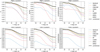 |
Fig. 1 f1 score (left), purity (middle), and completeness (right) versus limiting magnitude for the test sample. The thick solid lines show the performance of the combined algorithm, to be compared with the performance of the individual classifiers (thin lines). The vertical dotted lines show the magnitude limit of the miniJPAS survey (Bonoli et al. 2021). The top panel shows the performance for high-z quasars (with z ≥ 2.1) and the bottom panel the performance for low-z quasars (with z < 2.1). We see that the combined algorithm outperforms the rest. |
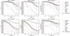 |
Fig. 2 Same as Figure 1 but for the test 1 deg2 sample. To aid with the visual comparison, we also add the performance of the combined algorithm in the test sample as a dashed line. |
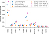 |
Fig. 3 Feature importance analysis of the combined algorithm classifier based on a modified version of the permutation feature importance technique (see text for details). The y-axis shows the feature importance for different scorers (f1 score, purity, and completeness), and for high-z and low-z quasars separately. These should be compared with the performance values listed in Table 3. Columns rSDSS, QPz, and LePhare are not included in our final classifier. |
4.3 Redshift precision
We now analyse the precision of our redshift estimate. We remind the reader that, as is described in Section 3, in normal operations, we only compute redshift estimates for objects classified as quasars. However, here we analyse the results of applying the redshift estimator to all the quasars of the test sample, irrespective of their classification. This helps to disentangle the effect of mistakes in the classification from the actual precision of our redshift estimates.
Figure 4 shows the distribution of the error in redshift given as Δz = ztrue − z, where ztrue is the ‘true’ redshift of the object, given in the truth table, and z is our redshift estimate. Besides the overall distribution, in Figure 4, we also show the distributions for high-z and low-z quasars separately, where the split is done based on the predicted redshifts (as opposed to using the preferred class). We also present a comparison with the distributions of the individual algorithms in Appendix C.
All three distributions are centred around zero, and we do not observe any systematic shift. However, we note a non-negligible amount of catastrophic errors in z, particularly for the low-z quasars. The redshift estimation for high-z quasars is typically more secure thanks to the presence of multiple emission lines, reducing the line confusion problem (i.e. correctly identifying an emission line but assigning the wrong label, and therefore a catastrophically different redshift)
To estimate the typical redshift uncertainty from this distribution, we used the normalised median absolute deviation, σNMAD, defined by Hoaglin et al. (1983) as
![Mathematical equation: $\[\sigma_{\mathrm{NMAD}}=1.48 \times \operatorname{median}\left(\frac{\left|k_{\operatorname{true}}-z\right|}{1+z_{\operatorname{true}}}\right).\]$](/articles/aa/full_html/2026/01/aa56424-25/aa56424-25-eq3.png) (3)
(3)
We obtain a value of σNMAD = 0.11 for the entire sample, σNMAD = 0.03 for high-z quasars, and σNMAD = 0.19 for low-z quasars. Indeed, this confirms that the redshift precision is much higher for high-z quasars. Again, having multiple emission lines helps secure the redshift information.
We compared the performance of the combined algorithm with that of the individual classifications: SQUEZE, QPz and LePhare. For the comparison with SQUEZE, we took its best classifications, i.e. z_SQUEZE_0, and we obtained σNMAD = 0.25, 0.27, and 0.19 for the entire sample, low-z quasars, and high-z quasars, respectively. Similarly, for QPz we obtained σNMAD = 0.21, 0.21, and 0.20, respectively, and for LePhare we obtained σNMAD = 0.83, 0.84, and 0.006, respectively. We see that, generally, the combined algorithm outperforms the rest of the algorithms. The exception to this is the obtained value of σNMAD for high-z quasars using LePhare. We note, however, that this comes at the cost of LePhare having a significantly worse performance, as is seen in the fraction of outliers (see bottom panel of Figure 5, and also the redshift distribution in Appendix C), which translates to an overall worse performance.
We further explore the evolution of the redshift error with the limiting magnitude in Figure 5. In the top panel, we see that for magnitudes fainter than r = 22, the measured σNMAD (solid line) is generally larger than the corresponding line obtained when analysing QPz results (dotted line), except when we include the faintest objects (with r ≳ 23.4). This increase in σNMAD can be explained by the inclusion of the other, less precise, redshift estimates. The benefit of adding these estimates can be seen in the bottom panel of Figure 5, showing a consistent decrease in the outlier fraction, i.e. the fraction of catastrophic redshift classifications (defined as objects with |Δz|/(1 + ztrue) > 0.15). In other words, the alternative redshift estimates, while not as precise as QPz, help alleviate the line confusion problem. As we mentioned before, for objects brighter than r = 22 we choose to keep QPz estimates as we otherwise see a similar increase in σNMAD without the benefit of decreasing the outlier fraction.
We close this section by performing a feature importance analysis on our redshift classifier. We followed the procedure described in Section 4.2 except that we changed the scoring functions. Because the scoring function needs to be maximised (i.e. larger scores are better), we chose to use −σNMAD as our scorer. We took three scores: one including all objects, one including high-z quasars only, and one including low-z quasars.
Results are given in Figure 6. We see that the dominant features are the redshift estimate from QPz and the classifications by CNN1, followed by the estimates from SQUEZE. We also see that LePhare estimates are the least relevant.
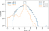 |
Fig. 4 Distribution of redshift errors for the test sample. The distribution, including all objects, is given in the black line. We also include the distributions for the high- and low-redshift split, respectively. The split was performed at z = 2.1 and considering the predicted redshift values. |
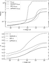 |
Fig. 5 Top panel: evolution of the measured σNMAD as a function of limiting magnitude. The solid line shows the results for our combined algorithm. The other lines show the measured σNMAD for QPz (dotted), the best estimate from SQUEZE (dashed), i.e. Z_SQUEZE_0, and LePhare (dash-dotted). The bottom panel shows the fraction of outliers, i.e. objects with |Δz|/(1 + ztrue) > 0.15, also as a function of limiting magnitude. We can see that, while the recovered σNMAD for the combined algorithm is sometimes larger than that of QPz, this is compensated by a decrease in the outlier fraction. |
5 Quasar catalogues
In Section 4, we have seen the performance of the combined algorithm on mock data. Now we apply it to the Mini J-PAS sources to build our final catalogues. For some applications, a more complete or purer catalogue is needed. Therefore, in our catalogues, we include all objects classified as quasars (irrespective of the classification confidence).
We built two catalogues. The first one includes only the point-like sources, including 784 sources. The second one also includes the extended sources and includes 11 487 sources. Here, it is worth stressing that the performance discussed in Section 4 applies to the point-like sources. The unreasonably large number of objects when including extended sources indicates that we cannot extend the usage of the combined algorithm beyond its training set, at least not in a straightforward manner. We provide the catalogue, including extended sources, as a bonus and at the user’s risk.
We show the number of quasars as a function of classification confidence in Figure 7. We take as classification confidence the highest confidence between the high-z and low-z quasar classes. As was expected, the number of quasars decreases with the classification confidence6. Analysing this figure, one can immediately see that there are way too many entries, especially when extended sources are included. This may suggest problems in our mocks that would impact the expected performance (this is further discussed in Section 6). We can, however, limit the number of objects by imposing confidence thresholds.
Results from Palanque-Delabrouille et al. (2016) predict the number of quasars up to magnitude r = 23 to be between 296 and 311, depending on the chosen luminosity model, of which between 81 and 91 are expected to be high-z quasars (see their table 5). Note that the numbers shown here include objects that go significantly fainter than this. If we restrict ourselves to objects brighter than r = 23, we are left with 533 entries in the point-like catalogue and 1824 when including the extended sources. For the point-like sample, imposing a confidence cut ≥0.65 reduces these numbers to a more sensible 300 quasars, of which 199 are high-z quasars. To achieve similar results when also including extended objects, we need to impose a confidence cut ≥0.85. In this case, we would obtain 307 quasars (51% of them are point-like sources), of which 230 have high-z (36% of them are point-like sources).
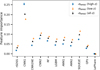 |
Fig. 6 Feature importance analysis of the combined algorithm redshift estimator based on a modified version of the permutation feature importance technique (see text for details). The y-axis shows the feature importance for the −σNMAD scorer. Different colours show the score for the entire sample (black), high-z quasars (orange), and low-z quasars (blue). These should be compared to the measured σNMAD = 0.11, 0.03 and 0.19, respectively. |
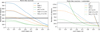 |
Fig. 7 Number of entries in our quasar catalogues as a function of classification confidence. The orange and green lines include the high-z and low-z entries, respectively. The blue lines are the sum of the orange and green lines. Solid lines include all the entries, irrespective of their magnitude, whilst the dashed lines exclude objects fainter than r = 23. Horizontal grey bands indicate the expected number of quasars down to magnitude r = 23 according to the models from Palanque-Delabrouille et al. (2016). The left panel shows the number of objects for the point-like catalogue, and the right panel also includes the extended sources. We note that in the bottom panel, the number of objects including all magnitudes is unreasonably large, and thus we choose to focus the y label on the magnitude-limited lines. |
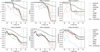 |
Fig. 8 Same as Figure 1 but for the DESI cross-match point-like sample. To aid with the visual comparison, we also add the performance of the combined algorithm in the test sample as a dashed line. |
6 Discussion
So far, we have shown that our combined algorithm outperforms the individual algorithms it was trained on. However, one of the main drawbacks of our analysis so far is that we completely rely on mocks for both training the algorithm and evaluating its performance. What is more, the number of quasars in our catalogues seems unrealistically large (although this issue can be mitigated by imposing a confidence cut). In previous papers of this series, we also argued that spectroscopic follow-up of the candidates is required to fully validate our findings (Rodrigues et al. 2023; Martínez-Solaeche et al. 2023; Pérez-Ràfols et al. 2023a).
Fortunately, with the publication of the DESI EDR, a fraction of our candidates have spectroscopic observations (see Section 2.2) that we visually inspected to assign labels (see Appendix A). Here, we used this sample to further probe the performance of the algorithm. We treated this sample as a truth table and computed the f1 score for the classification. The results of this exercise, considering only the point-like sources, are given in Figure 8 and summarised in Table 3.
Comparing this plot with Figures 1 and 2, we immediately see clear differences in the behaviour of the combined algorithm and the other classifiers. The most evident feature is that now the combined algorithm does not outperform the other algorithms. This can be explained by a drop in the performance of the CNN1 algorithm, particularly concerning the achieved purity. As we saw in Section 4, the combined algorithm is dominated by the classifications by CNN1 (see Figure 3).
In addition, we see that the change in performance is very algorithm-dependent. At a magnitude cut of r = 23.6, and compared to the performance on the test 1 deg2 sample, we see a decrease in the f1 score for high-z quasars of 0.11 for CNN1, 0.07 for the CNN2, and 0.17 for the combined algorithm. For other algorithms, we see instead an increase in performance. From larger to smaller increases, we have 0.29 for SQUEZE, 0.27 for RF, 0.17 for ANN2, 0.12 for LGBM, 0.10 for CNN1NE, and 0.06 for ANN1. For low-z quasars, we see a general increase in the performance. Again from larger to smaller increases in the f1 score, we have 0.43 for SQUEZE, 0.36 for LGBM, 0.35 for RF, 0.34 for CNN2, 0.33 for CNN1NE, 0.30 for ANN2, 0.25 for ANN1, and 0.23 for CNN1 and the combined algorithm.
It is worth noting that our mocks were created using SDSS spectra (Queiroz et al. 2023) and that DESI data are deeper. Mock objects that are fainter than the SDSS limit are thus drawn from brighter objects to which extra noise is added. Alas, we know the quasar properties to vary with magnitude (e.g. the Baldwin effect Baldwin 1977). Considering all this together, these results indicate that our mocks are not realistic enough, and a refined version is necessary. The different performances of the different algorithms are also suggestive of their potential overfitting and their resilience. Algorithms like SQUEZE, which rely on higher-level metrics for the classification, are suppressed in the combined algorithm due to their worse performance in mocks but have the greatest increase in performance when confronted with real data. Thus, once a new, more refined version of the mocks becomes available and the combined algorithm is retrained, we expect to see a significantly different feature importance analysis.
We now turn our attention to the performance of our redshift estimates. As we mentioned in Section 3, we only ran our redshift estimates in objects classified as quasars. Because we had already determined that the combined algorithm should not be used in extended sources, we studied the redshift precision only for the sample in the DESI cross-match point-like.
We see the results of this exercise in Figure 9. We get an overall σNMAD = 0.02 to be compared with the previous value of 0.11 estimated using mocks. The fraction of outliers is also generally smaller in real data than in mocks. We again see clear differences in the behaviour of the combined algorithm and the other classifiers. One big difference when compared to the performance changes seen in the classifier is that the redshift precision is better in real data than in mocks. Nevertheless, this change in performance again suggests that our mocks are not realistic enough (as was discussed above).
7 Summary and conclusions
In previous papers in the series, we have presented several machine-learning algorithms to construct quasar catalogues based on the automatic identification of the objects. Here, we have presented an extra layer of machine learning to optimally combine the results from the individual algorithms. We have then tested the algorithm on mocks and on data from the DESI EDR. We now summarise our conclusions:
When applied to mocks, the combined algorithm outperforms the rest of the classifiers. This is quantified using the f1 score. For the test sample, we reach f1 = 0.88 (f1 = 0.79) for high-z (low-z) quasars brighter than r = 23.6. We need to increase the magnitude cut to r = 23.2 and r = 21.8, respectively, to reach f1 = 0.9;
A feature importance analysis reveals that the combined algorithm is dominated by the CNN1 code, to which small adjustments are made based on the results from other codes (in particular the CNN2 and the ANN1);
When applied to data observed in DESI EDR, we find significant differences in the performance. This statement holds for both the combined algorithm and the individual classifiers. We note that for some algorithms, the performance increases, and for others, it decreases. In this case, the combined algorithm does not outperform the rest. We conclude that this signals an issue with the mocks themselves (and not the training of the combined algorithm). New, improved mocks are required in order to fix this issue;
We provide redshift estimates for our quasars. Based on mocks, we find a typical error of σNMAD = 0.18, but it seems to be much smaller than this when applied to data observed in DESI EDR, σNMAD = 0.02;
We provide a list of quasar candidates in the miniJPAS field with the associated confidence of classification. A confidence cut of 0.67 recovers a reasonable number of candidates;
The combined algorithm was trained using point-like sources. It cannot be applied to extended data with similar performance levels. We note, however, that a few quasars are observed as extended sources. To recover them, this should be taken into account in the mocks.
Data availability
The quasar catalogues are available at the CDS via https://cdsarc.cds.unistra.fr/viz-bin/cat/J/A+A/705/A232
Acknowledgements
This paper has gone through an internal review by the J-PAS collaboration. Based on observations made with the JST/T250 telescope and JPCam at the Observatorio Astrofísico de Javalambre (OAJ), in Teruel, owned, managed, and operated by the Centro de Estudios de Física del Cosmos de Aragón (CEFCA). We acknowledge the OAJ Data Processing and Archiving Unit (UPAD) for reducing and calibrating the OAJ data used in this work. Funding for the J-PAS Project has been provided by the Governments of Spain and Aragón through the Fondo de Inversiones de Teruel; the Aragonese Government through the Research Groups E96, E103, E16_17R, E16_20R, and E16_23R; the Spanish Ministry of Science and Innovation (MCIN/AEI/10.13039/501100011033 y FEDER, Una manera de hacer Europa) with grants PID2021-124918NB-C41, PID2021-124918NB-C42, PID2021-124918NA-C43, and PID2021-124918NB-C44; the Spanish Ministry of Science, Innovation and Universities (MCIU/AEI/FEDER, UE) with grants PGC2018-097585-B-C21 and PGC2018-097585-B-C22; the Spanish Ministry of Economy and Competitiveness (MINECO) under AYA2015-66211-C2-1-P, AYA2015-66211-C2-2, and AYA2012-30789; and European FEDER funding (FCDD10-4E-867, FCDD13-4E-2685). The Brazilian agencies FINEP, FAPESP, FAPERJ and the National Observatory of Brazil have also contributed to this project. Additional funding was provided by the Tartu Observatory and by the J-PAS Chinese Astronomical Consortium. IPR was supported by funding from the European Union’s Horizon 2020 research and innovation programme under the Marie Sklodowskja-Curie grant agreement No. 754510, and by the grant PID2023-151122NA-I00 by MICIU/AEI/10.13039/501100011033 and by ERDF/EU. RA is supported by the FAPESP grant 2022/03426-8. GMR and RMGD acknowledge financial support from the Severo Ochoa grant CEX2021-001131-S, funded by MICIU/AEI/10.13039/501100011033. They are also grateful for financial support from project PID2022-141755NB-I00, and project ref. AST22_00001_Subp 26 and 11, with funding from the European Union – NextGenerationEU. MMP was supported by the French National Research Agency (ANR) under contract ANR-22-CE31-0026 and by Programme National Cosmologie et Galaxies (PNCG) of CNRS/INSU with INP and IN2P3, co-funded by CEA and CNES. VM thanks CNPq (Brazil) and FAPES (Brazil) for partial financial support. LSJ acknowledges the support from CNPq (308994/2021-3) and FAPESP (2011/51680-6).
References
- Alexander, D. M., Davis, T. M., Chaussidon, E., et al. 2023, AJ, 165, 124 [NASA ADS] [CrossRef] [Google Scholar]
- Almeida, A., Anderson, S. F., Argudo-Fernández, M., et al. 2023, ApJS, 267, 44 [NASA ADS] [CrossRef] [Google Scholar]
- Arnouts, S., & Ilbert, O. 2011, LePHARE: Photometric Analysis for Redshift Estimate, Astrophysics Source Code Library [record ascl:1108.009] [Google Scholar]
- Bai, Y., Liu, J., Wang, S., & Yang, F. 2019, AJ, 157, 9 [Google Scholar]
- Baldwin, J. A. 1977, ApJ, 214, 679 [NASA ADS] [CrossRef] [Google Scholar]
- Baqui, P. O., Marra, V., Casarini, L., et al. 2021, A&A, 645, A87 [EDP Sciences] [Google Scholar]
- Benitez, N., Dupke, R., Moles, M., et al. 2014, arXiv e-prints [arXiv:1403.5237] [Google Scholar]
- Bertin, E., & Arnouts, S. 1996, A&AS, 117, 393 [Google Scholar]
- Bolzonella, M., Miralles, J. M., & Pelló, R. 2000, A&A, 363, 476 [NASA ADS] [Google Scholar]
- Bonoli, S., Marín-Franch, A., Varela, J., et al. 2021, A&A, 653, A31 [NASA ADS] [CrossRef] [EDP Sciences] [Google Scholar]
- Breiman, L. 1996, Mach. Learn., 24, 123 [Google Scholar]
- Breiman, L. 2001, Mach. Learn., 45, 5 [Google Scholar]
- Brodzeller, A., Wolfson, M., Santos, D. M., et al. 2025, Phys. Rev. D, 112, 083510 [Google Scholar]
- Chambers, K. C., Magnier, E. A., Metcalfe, N., et al. 2016, arXiv e-prints [arXiv:1612.05560] [Google Scholar]
- Chen, T., & Guestrin, C. 2016, in Proceedings of the 22nd ACM SIGKDD International Conference on Knowledge Discovery and Data Mining, KDD ’16 (New York, NY, USA: ACM), 785 [Google Scholar]
- Cirasuolo, M., Afonso, J., Bender, R., et al. 2011, The Messenger, 145, 11 [Google Scholar]
- Dalton, G., Trager, S., Abrams, D. C., et al. 2016, SPIE Conf. Ser., 9908, 99081G [Google Scholar]
- Dark Energy Survey Collaboration (Abbott, T., et al.) 2016, MNRAS, 460, 1270 [Google Scholar]
- de Jong, R. S. 2019, Nat. Astron., 3, 574 [NASA ADS] [CrossRef] [Google Scholar]
- DESI Collaboration (Aghamousa, A., et al.) 2016a, arXiv e-prints [arXiv:1611.00036] [Google Scholar]
- DESI Collaboration (Aghamousa, A., et al.) 2016b, arXiv e-prints [arXiv:1611.00037] [Google Scholar]
- DESI Collaboration (Adame, A. G., et al.) 2024, AJ, 168, 58 [NASA ADS] [CrossRef] [Google Scholar]
- DESI Collaboration (Adame, A. G., et al.) 2025, JCAP, 2025, 124 [CrossRef] [Google Scholar]
- Dewdney, P. E., Hall, P. J., Schilizzi, R. T., & Lazio, T. J. L. W. 2009, IEEE Proce., 97, 1482 [Google Scholar]
- Dey, A., Schlegel, D. J., Lang, D., et al. 2019, AJ, 157, 168 [Google Scholar]
- Euclid Collaboration (Mellier, Y., et al.) 2025, A&A, 697, A1 [Google Scholar]
- He, Z., Qiu, B., Luo, A. L., et al. 2021, MNRAS, 508, 2039 [NASA ADS] [CrossRef] [Google Scholar]
- Hoaglin, D. C., Mosteller, F., & Tukey, J. W. 1983, Understanding robust and exploratory data anlysis (Wiley) [Google Scholar]
- Ivezić, Ž., Kahn, S. M., Tyson, J. A., et al. 2019, ApJ, 873, 111 [Google Scholar]
- Jensen, T. W., Vivek, M., Dawson, K. S., et al. 2016, ApJ, 833, 199 [NASA ADS] [CrossRef] [Google Scholar]
- Kollmeier, J. A., Zasowski, G., Rix, H.-W., et al. 2017, arXiv e-prints [arXiv:1711.03234] [Google Scholar]
- Krakowski, T., Małek, K., Bilicki, M., et al. 2016, A&A, 596, A39 [NASA ADS] [CrossRef] [EDP Sciences] [Google Scholar]
- Kraljic, K., Laigle, C., Pichon, C., et al. 2022, MNRAS, 514, 1359 [NASA ADS] [CrossRef] [Google Scholar]
- Lan, T.-W., Tojeiro, R., Armengaud, E., et al. 2023, ApJ, 943, 68 [NASA ADS] [CrossRef] [Google Scholar]
- Levi, M., Bebek, C., Beers, T., et al. 2013, arXiv e-prints [arXiv:1308.0847] [Google Scholar]
- Logan, C. H. A., & Fotopoulou, S. 2020, A&A, 633, A154 [NASA ADS] [CrossRef] [EDP Sciences] [Google Scholar]
- López-Sanjuan, C., Varela, J., Cristóbal-Hornillos, D., et al. 2019, A&A, 631, A119 [Google Scholar]
- Lyke, B. W., Higley, A. N., McLane, J. N., et al. 2020, ApJS, 250, 8 [NASA ADS] [CrossRef] [Google Scholar]
- Martínez-Solaeche, G., Queiroz, C., González Delgado, R. M., et al. 2023, A&A, 673, A103 [NASA ADS] [CrossRef] [EDP Sciences] [Google Scholar]
- Merloni, A. 2016, in Lecture Notes in Physics 905, eds. F. Haardt, V. Gorini, U. Moschella, A. Treves, & M. Colpi (Berlin: Springer Verlag), 101 [Google Scholar]
- Morrison, S., Som, D., Pieri, M. M., Pérez-Ràfols, I., & Blomqvist, M. 2024, MNRAS, 532, 32 [Google Scholar]
- Palanque-Delabrouille, N., Magneville, C., Yèche, C., et al. 2016, A&A, 587, A41 [NASA ADS] [CrossRef] [EDP Sciences] [Google Scholar]
- Pedregosa, F., Varoquaux, G., Gramfort, A., et al. 2011, J. Mach. Learn. Res., 12, 2825 [Google Scholar]
- Pérez-Ràfols, I. & Pieri, M. M. 2020, MNRAS, 496, 4941 [CrossRef] [Google Scholar]
- Pérez-Ràfols, I., Pieri, M. M., Blomqvist, M., Morrison, S., & Som, D. 2020, MNRAS, 496, 4931 [CrossRef] [Google Scholar]
- Pérez-Ràfols, I., Abramo, L. R., Martínez-Solaeche, G., et al. 2023a, A&A, 678, A144 [NASA ADS] [CrossRef] [EDP Sciences] [Google Scholar]
- Pérez-Ràfols, I., Pieri, M. M., Blomqvist, M., et al. 2023b, MNRAS, 524, 1464 [Google Scholar]
- Queiroz, C., Abramo, L. R., Rodrigues, N. V. N., et al. 2023, MNRAS, 520, 3476 [Google Scholar]
- Ravoux, C., Armengaud, E., Walther, M., et al. 2020, JCAP, 2020, 010 [CrossRef] [Google Scholar]
- Rodrigues, N. V. N., Raul Abramo, L., Queiroz, C., et al. 2023, MNRAS, 520, 3494 [NASA ADS] [CrossRef] [Google Scholar]
- Salvato, M., Buchner, J., Budavári, T., et al. 2018, MNRAS, 473, 4937 [Google Scholar]
- Saxena, A., Salvato, M., Roster, W., et al. 2024, A&A, 690, A365 [NASA ADS] [CrossRef] [EDP Sciences] [Google Scholar]
- Storey-Fisher, K., Hogg, D. W., Rix, H.-W., et al. 2024, ApJ, 964, 69 [NASA ADS] [CrossRef] [Google Scholar]
- Takada, M., Ellis, R. S., Chiba, M., et al. 2014, PASJ, 66, R1 [Google Scholar]
- Wu, Q., & Shen, Y. 2022, ApJS, 263, 42 [NASA ADS] [CrossRef] [Google Scholar]
- Xiao-Qing, W., & Jin-Meng, Y. 2021, Chinese J. Phys., 69, 303 [NASA ADS] [CrossRef] [Google Scholar]
- Yip, C. W., Connolly, A. J., Vanden Berk, D. E., et al. 2004, AJ, 128, 2603 [Google Scholar]
Available on https://archive.cefca.es/catalogues/minijpas-pdr201912
Here, “easier” is ill-defined. It broadly refers to quasars with a larger number of emission lines and/or higher signal-to-noise.
Note that we expect the classification of high-z quasars to be easier as they typically contain a larger number of emission line features.
While the number of objects increases with magnitude, this is only true down to the limiting magnitude of the survey (included in our mocks). Only a small number of objects will go beyond this limit due to noise.
Naturally, a minimum confidence of 0.25 arises given that we are choosing from four classes.
Appendix A Visual inspection of DESI EDR objects
We visually inspected the 3720 DESI EDR objects with miniJPAS counterparts to search for potential flaws in the automatic classification. Each spectrum is evaluated using the Prospect tool7, which is the same tool used by DESI (Alexander et al. 2023; Lan et al. 2023). At least two people examined each spectrum and determined the quality of the automatic classification. Whenever there was disagreement between the inspectors, a final independent inspector examined the spectrum and made the final decision. We did not find a case where the final inspector was not in agreement with one of the previous inspections.
Since we are interested in the bulk classification between stars, galaxies, low-z quasars and high-z quasars, we did not refine the redshift estimates and only corrected them whenever we found a catastrophic error in their estimation. Of particular note is the classification of AGNs, where we also see the galactic emission. We classified them as quasars as long as we could observe the presence of a broad MgII line, irrespective of the strength of the galactic component.
We find a total of 667 stars, 2873 galaxies, 57 high-z quasars and 133 low-z quasars. We recover 4 high-z quasars and 23 low-z quasars. Most of the recovered low-z quasars are indeed these AGNs, where we detect the galactic emission. We note that DESI corrects the automatic classification by Redrock with the usage of afterburners to recover these objects (Alexander et al. 2023). Having analysed this sample, we confirm that the DESI automatic pipeline performs excellently, missing only a small number of quasars.
Appendix B Samples comparison
One of the main findings in section 6 is that all our algorithms have different performance on mocks compared to the performance on data. Some of the algorithms perform worse when run on data, and some have better performance. What is more, we argue that our mocks are not realistic enough. Here we present a more detailed comparison between the different samples. Figure B.1 shows a comparison of the magnitude distribution of the samples, where we see that the magnitude distributions are very different.
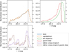 |
Fig. B.1 Normalised magnitude distribution for the different samples. For guidance, the peak of the distribution in the mock samples is shown as vertical dashed lines in all the panels. We see significant variations of the distributions. |
Appendix C Distribution of redshift errors
In section 4.3 we analysed the redshift precision of the combined algorithm. In particular, we showed the distribution of redshift errors for the test sample in figure 4. Here, we compare those distributions with the equivalent distributions for the individual classifiers. This is shown in figure C.1 for all quasars (top panel), high-z quasars (mid panel) and low-z quasars (bottom panel).
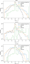 |
Fig. C.1 Distribution of redshift errors for the test sample for the different classifiers. The top panel show the distribution for all quasars, and the middle and bottom panels show the distributions for the high/low redshift split. The split is performed at z = 2.1 and considering the predicted redshift values. |
We see that the distribution for the combined algorithm has thinner wings, compared to the SQUEZE and QPz. This indicates that by combining the results, we are improving our classifications by reducing the number of catastrophic errors. We can also see that LePhare has a large fraction of catastrophic redshifts, as seen also in the large fraction of outliers in figure 5. Here, we see that this effect is larger for (but not limited to) low-z quasars.
Appendix D Data model for catalogue files
Data in the quasar catalogue is provided in compressed FITS files (.fits.gz) in a single Header Data Unit. For each entry, we provide both our final classification and the classification from the individual algorithms. Details on the columns are given in table D.1.
Column description in the data format.
All Tables
All Figures
|
Fig. 1 f1 score (left), purity (middle), and completeness (right) versus limiting magnitude for the test sample. The thick solid lines show the performance of the combined algorithm, to be compared with the performance of the individual classifiers (thin lines). The vertical dotted lines show the magnitude limit of the miniJPAS survey (Bonoli et al. 2021). The top panel shows the performance for high-z quasars (with z ≥ 2.1) and the bottom panel the performance for low-z quasars (with z < 2.1). We see that the combined algorithm outperforms the rest. |
| In the text | |
|
Fig. 2 Same as Figure 1 but for the test 1 deg2 sample. To aid with the visual comparison, we also add the performance of the combined algorithm in the test sample as a dashed line. |
| In the text | |
|
Fig. 3 Feature importance analysis of the combined algorithm classifier based on a modified version of the permutation feature importance technique (see text for details). The y-axis shows the feature importance for different scorers (f1 score, purity, and completeness), and for high-z and low-z quasars separately. These should be compared with the performance values listed in Table 3. Columns rSDSS, QPz, and LePhare are not included in our final classifier. |
| In the text | |
|
Fig. 4 Distribution of redshift errors for the test sample. The distribution, including all objects, is given in the black line. We also include the distributions for the high- and low-redshift split, respectively. The split was performed at z = 2.1 and considering the predicted redshift values. |
| In the text | |
|
Fig. 5 Top panel: evolution of the measured σNMAD as a function of limiting magnitude. The solid line shows the results for our combined algorithm. The other lines show the measured σNMAD for QPz (dotted), the best estimate from SQUEZE (dashed), i.e. Z_SQUEZE_0, and LePhare (dash-dotted). The bottom panel shows the fraction of outliers, i.e. objects with |Δz|/(1 + ztrue) > 0.15, also as a function of limiting magnitude. We can see that, while the recovered σNMAD for the combined algorithm is sometimes larger than that of QPz, this is compensated by a decrease in the outlier fraction. |
| In the text | |
|
Fig. 6 Feature importance analysis of the combined algorithm redshift estimator based on a modified version of the permutation feature importance technique (see text for details). The y-axis shows the feature importance for the −σNMAD scorer. Different colours show the score for the entire sample (black), high-z quasars (orange), and low-z quasars (blue). These should be compared to the measured σNMAD = 0.11, 0.03 and 0.19, respectively. |
| In the text | |
|
Fig. 7 Number of entries in our quasar catalogues as a function of classification confidence. The orange and green lines include the high-z and low-z entries, respectively. The blue lines are the sum of the orange and green lines. Solid lines include all the entries, irrespective of their magnitude, whilst the dashed lines exclude objects fainter than r = 23. Horizontal grey bands indicate the expected number of quasars down to magnitude r = 23 according to the models from Palanque-Delabrouille et al. (2016). The left panel shows the number of objects for the point-like catalogue, and the right panel also includes the extended sources. We note that in the bottom panel, the number of objects including all magnitudes is unreasonably large, and thus we choose to focus the y label on the magnitude-limited lines. |
| In the text | |
|
Fig. 8 Same as Figure 1 but for the DESI cross-match point-like sample. To aid with the visual comparison, we also add the performance of the combined algorithm in the test sample as a dashed line. |
| In the text | |
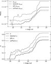 |
Fig. 9 Same as Figure 5 but for the DESI cross-match point-like sample. |
| In the text | |
|
Fig. B.1 Normalised magnitude distribution for the different samples. For guidance, the peak of the distribution in the mock samples is shown as vertical dashed lines in all the panels. We see significant variations of the distributions. |
| In the text | |
|
Fig. C.1 Distribution of redshift errors for the test sample for the different classifiers. The top panel show the distribution for all quasars, and the middle and bottom panels show the distributions for the high/low redshift split. The split is performed at z = 2.1 and considering the predicted redshift values. |
| In the text | |
Current usage metrics show cumulative count of Article Views (full-text article views including HTML views, PDF and ePub downloads, according to the available data) and Abstracts Views on Vision4Press platform.
Data correspond to usage on the plateform after 2015. The current usage metrics is available 48-96 hours after online publication and is updated daily on week days.
Initial download of the metrics may take a while.