| Issue |
A&A
Volume 705, January 2026
|
|
|---|---|---|
| Article Number | A33 | |
| Number of page(s) | 14 | |
| Section | Extragalactic astronomy | |
| DOI | https://doi.org/10.1051/0004-6361/202556485 | |
| Published online | 07 January 2026 | |
The Galaxy Activity, Torus, and Outflow Survey (GATOS)
X. Molecular gas clumpiness under the influence of AGN
1
Observatorio de Madrid, OAN-IGN, Alfonso XII, 3, E-28014 Madrid, Spain
2
Centro de Astrobiología (CAB, CSIC-INTA), Camino Bajo del Castillo s/n, E-28692 Villanueva de la Cañada, Madrid, Spain
3
Observatoire de Paris, LUX, PSL University, Sorbonne Université, CNRS, F-75014 Paris, France
4
Collège de France, 11 Place Marcelin Berthelot, 75231 Paris, France
5
Max-Planck-Institut für Extraterrestrische Physik, Postfach 1312, 85741 Garching, Germany
6
Department of Physics & Astronomy, University of South Carolina, Columbia, SC 29208, USA
7
Kavli Institute for Particle Astrophysics & Cosmology (KIPAC), Stanford University, Stanford, CA 94305, USA
8
Instituto de Radioastronomía y Astrofísica (IRyA-UNAM), Antigua Carretera a Pátzcuaro #8701 Ex-Hda. San José de la Huerta, C.P., 58089 Morelia, Michoacán, Mexico
9
Instituto de Astrofísica de Canarias (IAC), Calle Vía Láctea s/n, 38205 La Laguna, Tenerife, Spain
10
Departamento de Astrofísica, Universidad de La Laguna, 38206 La Laguna, Tenerife, Spain
11
Department of Physics & Astronomy, University of Alaska Anchorage, Anchorage, AK 99508-4664, USA
12
Department of Astronomy, University of Geneva, 1290 Versoix, Switzerland
13
Instituto de Estudios Astrofísicos, Facultad de Ingeniería y Ciencias, Universidad Diego Portales, Av. Ejército Libertador 441, Santiago, Chile
14
Departamento de Física de la Tierra y Astrofísica, Fac. de CC. Físicas, Universidad Complutense de Madrid, 28040 Madrid, Spain
15
Instituto de Física de Partículas y del Cosmos IPARCOS, Universidad Complutense de Madrid, 28040 Madrid, Spain
16
Cahill Center for Astrophysics, California Institute of Technology, 1216 East California Boulevard, Pasadena, CA 91125, USA
17
Department of Physics, University of Oxford, Denys Wilkinson Building, Keble Road, Oxford OX13RH, UK
18
School of Mathematics, Statistics and Physics, Newcastle University, Newcastle upon Tyne NE1 7RU, UK
19
Institute of Astrophysics, Foundation for Research and Technology – Hellas (FORTH), Voutes 70013 Heraklion, Greece
20
School of Sciences, European University Cyprus, Diogenes street, Engomi, 1516 Nicosia, Cyprus
21
School of Physics & Astronomy, University of Southampton, Southampton, SO17 1BJ Hampshire, UK
22
Telespazio UK for the European Space Agency (ESA), ESAC, Camino Bajo del Castillo s/n, 28692 Villanueva de la Cañada, Madrid, Spain
23
Space Telescope Science Institute, 3700 San Martin Drive Baltimore, MD 21218, USA
24
Department of Physics and Astronomy, The University of Texas at San Antonio, 1 UTSA Circle, San Antonio, TX 78249, USA
25
Instituto de Física Fundamental, CSIC, Calle Serrano 123, 28006 Madrid, Spain
26
Centro de Astrobiología (CAB, CSIC/INTA), Ctra de Torrejón a Ajalvir, km 4, 28850 Torrejón de Ardoz, Madrid, Spain
27
Departamento de Física, CCNE, Universidade Federal de Santa Maria, Av. Roraima 1000, 97105-900 Santa Maria, RS, Brazil
★ Corresponding author: This email address is being protected from spambots. You need JavaScript enabled to view it.
Received:
18
July
2025
Accepted:
17
October
2025
Abstract
The distribution of molecular gas on small scales regulates star formation and the growth of supermassive black holes in galaxy centers. Yet, the role of active galactic nuclei (AGN) feedback in shaping this distribution remains poorly constrained. We investigate how AGNs influence the small-scale structure of molecular gas in galaxy centers by measuring the clumpiness of CO(3 − 2) emission observed with the Atacama Large Millimeter/submillimeter Array (ALMA) in the nuclear regions (50 − 200 pc from the AGNs) of 16 nearby Seyfert galaxies from the Galaxy Activity, Torus, and Outflow Survey (GATOS). To quantify clumpiness we applied three different methods: (1) the median of the pixel-by-pixel contrast between the original and smoothed maps; (2) the ratio of the total excess flux to the total flux, after subtracting the background smoothed emission; and (3) the fraction of total flux coming from clumpy regions, interpreted as the mass fraction in clumps. We find a negative correlation between molecular gas clumpiness and AGN X-ray luminosity (LX), suggesting that higher AGN activity is associated with smoother gas distributions. All methods reveal a turnover in this relation around LX = 1042 erg s−1, possibly indicating a threshold above which AGN feedback becomes efficient at dispersing dense molecular structures and suppressing future star formation. Our findings provide new observational evidence that AGN feedback can smooth out dense gas structures in galaxy centers.
Key words: evolution / ISM: structure / galaxies: active / galaxies: ISM / galaxies: nuclei
© The Authors 2026
 Open Access article, published by EDP Sciences, under the terms of the Creative Commons Attribution License (https://creativecommons.org/licenses/by/4.0), which permits unrestricted use, distribution, and reproduction in any medium, provided the original work is properly cited.
This article is published in open access under the Subscribe to Open model. This email address is being protected from spambots. You need JavaScript enabled to view it. to support open access publication.
1. Introduction
Active galactic nuclei (AGNs) are powerful sources of energy and momentum that can significantly impact the interstellar medium (ISM) of their host galaxies. The feedback processes driven by AGNs, including both radiative and mechanical effects, play a crucial role in shaping gas distribution, star formation, and the overall evolution of galaxies (Fabian 2012; Kormendy & Ho 2013; Heckman & Best 2014; Morganti 2017; Harrison et al. 2018). Deciphering the mechanisms by which AGN feedback affects the ISM and drives galaxy evolution is one of the major challenges in modern astrophysics (see Harrison & Ramos Almeida 2024, for a recent review).
Within a galaxy molecular gas can organize into giant molecular clouds (GMCs), with typical masses MGMC ∼ 104 − 106 M⊙ and sizes of ∼10 − 50 pc (Solomon et al. 1987; Omont 2007; Fukui & Kawamura 2010; Heyer & Dame 2015; Chevance et al. 2020, 2023). Such clouds are sufficiently massive and dense that their self-gravity tends to drive gravitational collapse. However, GMCs can achieve a quasi-stable state because other internal forces – mainly magnetic pressure and turbulent motions – provide support that counteracts collapse (McKee & Ostriker 2007; Crutcher 2012). Within them there exists a complex hierarchical structure of progressively smaller high-density structures (Elmegreen & Falgarone 1996; Federrath & Klessen 2012; Elia et al. 2018; Buck et al. 2022), which are thought to be the sites of star formation (Bergin & Tafalla 2007; Heyer & Dame 2015; Massi et al. 2019).
Active galactic nuclei-driven radiation, winds, jets, and cosmic rays can further compress, evaporate, or disperse gas (Pier & Voit 1995; Schartmann et al. 2011; Namekata et al. 2014; Pozzi et al. 2017; Vallini et al. 2017; Mingozzi et al. 2018; Circosta et al. 2021; Gabici 2022; Bertola et al. 2024; Koutsoumpou et al. 2025), and although there are hints of positive feedback (e.g., Maiolino et al. 2017; Bessiere & Ramos Almeida 2022; Mercedes-Feliz et al. 2023), we mostly observe molecular gas depletion in the central regions of active galaxies (Sabatini et al. 2018; Rosario et al. 2019; Ellison et al. 2021; García-Burillo et al. 2021, 2024). Among the clearest signatures of AGN impact on the host ISM, García-Burillo et al. (2021, 2024) reported a systematic deficit in the central concentration of cold molecular gas in AGN-host galaxies, quantified through the concentration index log(Σ50/Σ200), where Σ50 and Σ200 are the average CO surface densities within circular apertures of 50 pc and 200 pc radii, respectively. They found that this concentration index shows a turnover as a function of AGN X-ray luminosity, with a change around LX(2 − 10 keV)∼1041.5 erg s−1. While the concentration index quantifies how centrally peaked the gas distribution is, it does not capture the small-scale structure within the nuclear region. In this work we focus on the clumpiness of the molecular gas, a property that reflects how fragmented or structured the emission is within the nuclear region.
Molecular gas clumpiness, characterized by an irregular and dense distribution, can serve as an indirect measure of star formation activity, as the most clumpy regions lie where the gravitational collapse leads to the formation of new stars (Krumholz 2014; Krumholz et al. 2019). Understanding the potential role that AGN feedback plays in shaping the molecular gas clumpiness of their host galaxies is crucial for assessing how AGN can regulate star formation and the evolution of galaxy centers. To this end this work is part of the Galaxy Activity, Torus, and Outflow Survey (GATOS1, García-Burillo et al. 2021; Alonso-Herrero et al. 2021; García-Bernete et al. 2024a,b; Zhang et al. 2024; Poitevineau et al. 2025; Fuller et al. 2025), an ongoing effort to study the properties of AGN, dusty molecular tori, and AGN interaction with the host galaxy in local Seyfert galaxies using high-resolution observations.
The paper is structured as follows: In Section 2 we introduce the sample of galaxies. In Section 3 we describe the methods for measuring clumpiness and the statistical tools employed in our analysis. Section 4 presents the results of our analysis, and in Section 5 we discuss the implications of our findings in the context of AGN feedback on the molecular gas. Finally, we summarize our conclusions in Section 6.
2. Sample description
The initial sample consists of 19 nearby (luminosity distance DL < 28 Mpc) AGNs, combining the NUGA sample (Nuclei of Galaxies, Combes et al. 2019; Audibert et al. 2019, 2021) with the core sample of GATOS galaxies presented in García-Burillo et al. (2021). The GATOS core sample was selected from the 70 month Swift-BAT all-sky hard-X ray survey (Baumgartner et al. 2013) with distances DL < 28 Mpc and luminosities L(14 − 150 keV)≥1042 erg s−1. The CO(3 − 2) data used here were analyzed in detail by García-Burillo et al. (2021), where moment maps and kinematic modeling are discussed. All galaxies have CO(3 − 2) emission observed with the Atacama Large Millimeter/submillimeter Array (ALMA) Band 7, covering a field of view of 17″, and spatial resolutions ranging from 0.08″ to 0.2″, corresponding to a physical size range of 4 − 16 pc.
Inclinations and position angles of the targets are taken from García-Burillo et al. (2021), which reported the results of a kinematical analysis performed with the kinemetry software (Krajnović et al. 2006). Since our goal is to study the clumpiness of the molecular gas, we decided to discard highly inclined (i > 75°) galaxies from the original sample. This decision was made to avoid severe projection effects, as high inclination makes it more likely for the line of sight to intersect multiple layers of clumps and diffuse gas. This selection results in a sample of 16 galaxies, all with inclinations i < 60°. Their intrinsic 2 − 10 keV luminosities span from 1039 to 1043.5 erg s−1, and their Eddington ratios, λEdd ≡ LAGN/LEdd, range from −6.4 to −0.7 in logarithmic scale. Table A.1 lists the basic properties of the galaxies analyzed in this study, and Figure A.3 presents an atlas of their CO(3 − 2) emission.
The sensitivity of the CO(3 − 2) maps ranges from 6 to 28 mJy km s−1 beam−1. We checked whether this sensitivity correlates with the luminosity distance of the galaxies and found no such trend (see Figure A.1). To express these values in terms of molecular mass surface density, we adopted reasonable conversion factors: first, from CO(3 − 2) to CO(1 − 0) (r31), then from CO(1 − 0) to molecular mass via the CO-to-H2 conversion factor (XCO). We explored two extreme cases. The first assumes r31 = 0.7, the average value measured by Israel (2020) in 126 galaxy centers, combined with the standard Milky Way disk value XCO = 2 × 10²⁰ mol cm−2 (K km s−1)−1 (Bolatto et al. 2013). The second adopts r31 = 2.9, as measured at the AGN position of NGC 1068 by Viti et al. (2014), coupled with the recommended value for the central region (R < 500 pc) of the Milky Way, XCO = 0.5 × 10²⁰ mol cm−2 (K km s−1)−1 (Bolatto et al. 2013). With the first set of parameters, the resulting sensitivities span 23 − 381 M⊙ pc−2, while with the second they range from 1 to 23 M⊙ pc−2 (see Figure A.2). The achieved sensitivities are generally comparable to, or lower than, the average surface density of GMCs (170 M⊙ pc−2, McKee & Ostriker 2007) and, in most cases, sufficient to detect individual GMCs within a single ALMA beam at the 3σ level.
3. Data analysis
3.1. Identifying the clumps
To visualize and measure the clumpiness of the molecular gas, we chose the clumpiness parameter described by Conselice (2003) among those available in the literature. Whereas Conselice (2003) originally estimated clumpiness (S), together with concentration (C) and asymmetry (A), from optical images tracing stellar light in entire galaxies – the so-called CAS parameters – this method has since been applied to ALMA CO(2 − 1) observations by Yamamoto et al. (2025), using data from the Physics at High Angular resolution in Nearby GalaxieS (PHANGS; Leroy et al. 2021) survey.
The method involves smoothing the original observation and subtracting the smoothed map (B, for blurred) from the original intensity map (I). This results in an I − B residual map, which highlights only the high-spatial frequency components of the original map. Negative pixels (where I − B < 0) are set to zero. The clumpiness parameter (S) calculated by Conselice (2003) is then normalized by the original intensity, S = (I − B)/I, so that it has a value between zero (indicating smooth emission, with no clumps) and one (indicating high clumpiness). In this work we followed the procedure outlined in Conselice (2003) to identify the clumps, defined as the pixels or contiguous regions where I − B > 0. We then applied three different methods to quantify the clumpiness of the gas, as described in the following sections. Before performing any analysis, we first smoothed all the CO maps to a common physical resolution of 16 pc, corresponding to the largest ALMA beam in the sample.
3.2. Smoothing CO(3–2) maps
A critical factor of the Conselice (2003) procedure is the size of the smoothing kernel. Ideally, we want the full width at half maximum (FWHM) of the kernel to be larger than the spatial resolution but smaller than the aperture we consider. Moreover, we expected the largest GMCs to have sizes of ≲100 pc (see, e.g., García et al. 2014), so smoothing over this size would result in blending several GMCs and diluting the high-density gas. Therefore, we use smoothing kernels with FWHM between 20 and 100 pc in the following analysis. We discuss the implications of different kernel sizes in Section 5.
An example of the full procedure can be seen in the four panels of Figure 1 for the galaxy NGC 3227. We first smoothed the native-resolution CO(3 − 2) emission map (first panel) with a 16 pc Gaussian kernel to bring all galaxies to a common physical resolution (second panel). This map was then smoothed again with a larger Gaussian kernel (50 pc in Figure 1), producing a version that traces the average gas distribution over the corresponding spatial scale (third panel). We subtracted this smoothed map from the 16 pc map and retained only the pixels with positive residuals (fourth panel; see details on how clumpiness is computed below). This procedure highlights the regions where the emission is significantly more concentrated than the surrounding gas distribution, identifying candidate clumps.
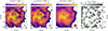 |
Fig. 1. ALMA observations of the CO(3 − 2) emission in the target galaxy NGC 3227 and the clumpiness computation applied within a 400 pc × 400 pc box around the AGN. First panel: CO(3 − 2) emission at native resolution (10.5 × 9.4 pc), with contours at (3, 5, 10, 20, 30, 50)×σ. Second panel: CO(3 − 2) emission smoothed to a common physical resolution of 16 pc, using contours at the same σ levels. Third panel: CO(3 − 2) emission further smoothed with a Gaussian kernel of FWHM 50 pc, with the same contour levels. Fourth panel: Clumpiness map computed with Method #1 (see Section 3.3), with contours every 0.1 from 0 to 1. In all panels the two ellipses correspond to circles with radii of 50 and 200 pc in the galaxy plane, projected onto the sky. The red ellipse within a square in the bottom right of each panel shows the native ALMA beam (10.5 × 9.4 pc in this case). |
3.3. Measuring nuclear and circumnuclear clumpiness
In contrast to distant quasars (see, e.g., Maiolino et al. 2012; Genzel et al. 2014; Carniani et al. 2017; Bischetti et al. 2019), nearby AGNs are generally found to primarily affect their host galaxies within the central kiloparsec, mainly due to their lower luminosities and outflow energetics (see, e.g., Querejeta et al. 2016a; Fluetsch et al. 2019; Esposito et al. 2022, 2024b,a; García-Bernete et al. 2021; Ramos Almeida et al. 2022; García-Burillo et al. 2021, 2024). In this work we follow García-Burillo et al. (2021, 2024) in defining two concentric regions centered on the AGN position (based on the ALMA continuum peak, see García-Burillo et al. 2021), with radii of 50 pc and 200 pc in the plane of the galaxy. These scales were previously adopted to compute the cold molecular gas concentration index (CCI ≡log(Σ50/Σ200)). We used inclinations and position angles to project these two circles onto the plane of the galaxy. An example of this can be seen in Figure 1, where the two ellipses are drawn on top of the CO(3 − 2) emission map. We explore three different methods for measuring the clumpiness within the 50 pc and 200 pc apertures.
3.3.1. Method #1: Median clumpiness
The first method follows that of Conselice (2003): we calculated the clumpiness as (I − B)/I pixel by pixel, setting negative pixels to zero, as shown in the fourth panel of Figure 1. We then took the median value of the clumpiness within the two apertures, referring to this method as “Method #1: median clumpiness”. To estimate the errors, we used the 1σ distance from the median values. This method provides a clumpiness value that can be compared with other studies (e.g., Conselice 2003; Yamamoto et al. 2025). However, high clumpiness values tend to identify regions with higher contrast, especially in the outskirts of the CO emission, rather than dense or massive clumps, as visible in Figure 1. For this reason, we sought alternative methods to estimate the fraction of gas in clumps.
3.3.2. Method #2: ΣI − B/Σtot
The second method is similar to Method #1 in principle, as it calculates the clumpiness as (I − B)/I. However, instead of computing it pixel by pixel and then taking the median value, we separately summed the I − B and I values within the apertures and then divided them. We call this method “Method #2: ΣI − B/Σtot”. Since CO intensity can be converted to molecular mass using a CO-to-H2 conversion factor αCO, and assuming the same αCO for both the clumpy emission and the underlying smooth emission, the result of ΣI − B/Σtot can be interpreted as the mass fraction of gas in clumps, independent of the choice of αCO. This method returns values between 0 and 1, where higher values indicate a greater contrast between clumpy and smooth gas. Since this method is analogous to aperture photometry, we used the photometric errors to estimate the uncertainties. For the ALMA observations, these are dominated by the calibration error, which can be as high as ∼10% (Francis et al. 2020). This results in a propagated uncertainty of ∼17%.
3.3.3. Method #3: Σclumps/Σtot
The third method uses the condition I − B > 0 to identify the clumps and sums the original pixel intensities I (without subtracting the smoothed B emission) to calculate the flux of the clumps, Σclumps, within the different apertures. We divided this by the total flux Σtot and refer to this as “Method #3: Σclumps/Σtot”. By not subtracting the smoothed emission, we aimed to obtain a more direct measurement of the fraction of molecular mass in clumps. As a result, this method tends to yield systematically higher clumpiness values compared to the other two. As with the second method, we assumed an approximate error of 10% on the flux measurements, which propagates to an approximate uncertainty of 14%.
These three methods are designed to capture complementary aspects of clumpiness, each with its own sources of systematic uncertainty. Using multiple approaches allows us to test the robustness of our results against these effects, rather than relying on a single estimator of clumpiness.
3.4. Estimating the influence of AGN on clumpiness
One of the most reliable indicators of the power of an AGN is its intrinsic 2 − 10 keV X-ray luminosity, LX, which serves as a proxy for both radiative feedback on the ISM (through the creation of X-ray dominated regions, or XDRs; see, e.g., Maloney et al. 1996; Wolfire et al. 2022; Esposito et al. 2024a; Tadaki et al. 2025) and mechanical feedback (through the interaction of AGN winds with the host galaxy’s ISM; see, e.g., Faucher-Giguère & Quataert 2012; Cicone et al. 2014; Nims et al. 2015; Fiore et al. 2017; Esposito et al. 2024b). We used LX as a measure of AGN power and investigated possible correlations between the AGN emission and our different clumpiness measurements, considering various smoothing kernels and aperture sizes. To do this we applied the piecewise linear fitting (PWLF) algorithm using the Python package pwlf (Jekel & Venter 2019), which fits continuous piecewise linear functions to the data based on a specified number of line segments. We began by fitting both a single-segment (i.e., standard linear regression) and a two-segment model. We then performed an F-test (at the 95% confidence level) to evaluate whether the two-segment model provides a statistically significant improvement over the single-segment model. If the two-segment fit was not preferred, we adopted the single-segment model and assessed the significance of its slope with a two-tailed t-test under the null hypothesis of zero slope.
For each dataset (i.e., a combination of clumpiness method, smoothing level, and aperture) where a two-segment fit was preferred, we tested for the presence of a break point–an LX value where the slope changes–using two statistical techniques. First, we performed leave-one-out cross-validation (LOOCV), iteratively excluding one data point at a time to examine the distribution of break points within the dataset. This helps assess whether the fit is significantly influenced by individual points. We consider a break point reliable only if the standard deviation of its LOOCV distribution is smaller than 10% of the LX-range of the data. Second, for each validated dataset, we ran 1000 Monte Carlo simulations, taking into account the data uncertainties in both axes: we assumed a ±0.15 dex uncertainty for LX (following García-Burillo et al. 2024); clumpiness uncertainties are described in Section 3.3. This approach allowed us to statistically confirm the presence of a break point and to estimate its 1σ confidence interval using Monte Carlo resampling.
4. Results
4.1. The nuclear region
Figure 2 shows the clumpiness, measured within the 50 pc radius aperture, as a function of the X-ray luminosity, LX, of our sample targets. Clumpiness is computed using the three methods described in Section 3.3, with the nine different smoothing levels applied, ranging from 20 to 100 pc in steps of 10 pc. This allows us to trace how clumpiness varies as a function of the smoothing scale.
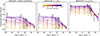 |
Fig. 2. Clumpiness as a function of AGN intrinsic X-ray 2 − 10 keV luminosity. Clumpiness is measured within the nuclear 50 pc radius aperture with the three different methods described in Section 3.3 (panels left to right). Data points (square markers, nine per galaxy) are colored according to the nine smoothing FWHM sizes adopted (see the color bar in the central panel). The colored lines show the pwlf fits to the data points, with the same color as the fitted dataset; the lines are solid where a linear fit is statistically accepted, and dashed where it is rejected (see Section 3.4). |
For each smoothing level, we fit the data using the PWLF algorithm and plot the corresponding regression lines. At low smoothing levels, when the kernel size is close to the ALMA beam, the clump identification condition (I − B > 0) primarily selects the peaks of the clumps. As a result, Methods #1 and #2 return values close to zero with no apparent break points in the fit. In contrast, Method #3 begins from a baseline value of Σclumps/Σtot ≈ 0.6, indicating that even at the smallest smoothing scales, clumps already contribute approximately 60% of the CO emission. In addition, Method #3 already shows a statistically significant break point at LX ∼ 1041.8 erg s−1 emerging from smoothing scales as small as 30 pc.
Up to a smoothing scale of 50 pc, the data show a significant (p < 0.05), weak (r2 < 0.4) anticorrelation between LX and clumpiness for Methods #1 and #2. As the smoothing level increases, a two-segment trend emerges also for these methods, with a relatively flat trend at the lowest luminosities, followed by a steep decline. The break point in these cases typically falls around LX ∼ 1041.5 erg s−1. The exact smoothing level required to reveal a significant break point depends on the method used: for Method #3, the trend appears at 30 pc; for Method #2, at 60 pc; and for Method #1, at 90 pc.
From a smoothing level of 90 pc, a two-segment fit appears for every method. Figure 3 shows the data points for this smoothing level, including error bars, the pwlf lines, and the 95% confidence interval from Monte Carlo simulations. For Method #1, the LOOCV algorithm finds a high standard deviation (30% of the LX range), indicating that the exact position of the LX break point is not well constrained and should be treated with caution. This is further illustrated in Figure 2, where at smoothing scales of 70 and 80 pc, the break point appears at very low LX ∼ 1039 erg s−1 – probably an artifact of the fitting process – before shifting to higher LX values at larger smoothing scales. The broad confidence interval in Figure 3 further reflects this uncertainty. In contrast, for Methods #2 and #3, the LOOCV validates the break points, with standard deviations of 7% and 1% of the LX range, respectively, yielding  and
and  .
.
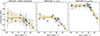 |
Fig. 3. Clumpiness as a function of AGN X-ray luminosity. Clumpiness is measured within the nuclear 50 pc radius aperture with the three different methods described in Section 3.3 (panels left to right). Data points are shown as blue square markers with error bars, computed for a smoothing kernel FWHM of 90 pc. The broken orange lines indicate the pwlf fits to the data, and the shaded regions indicate the corresponding 95% confidence intervals. |
It is interesting to note that, for both Methods #2 and #3, the break point position shifts to higher X-ray luminosity values as we increased smoothing: at 80 pc smoothing, we find the break points at  and
and  , respectively for Methods #2 and #3, while at 100 pc smoothing we find them at
  and
and  . Considering only Methods #2 and #3, we find that the break points are compatible with each other, given the uncertainties, to a value of LX ≈ 1042 erg s−1.
Finally, we explored the relation between clumpiness and the AGN Eddington ratio, λEdd, as shown in Figure A.5. We find a similar pattern (flat regime followed by a steep decline) by using Methods #1 and #3, with break points between λEdd = −3 and −2.
4.2. The circumnuclear region
Applying the same methods to the 200 pc aperture, we find significantly decreasing linear trends without break points for Methods #1 and #2. Method #3 also shows an anticorrelation between LX and clumpiness, but no smoothing kernel size yields a significance above 2σ (see Figure 4). Beyond physical explanations (discussed in Section 5), some targets in this aperture include regions dominated by noise or empty space (e.g., NGC 7213 and NGC 1365; see Figure A.3), which may affect the analysis. When considering only the annular region between galactocentric distances of 50 pc and 200 pc, we obtain less significant results, likely due to the high noise present in this annular aperture (see Figure A.6).
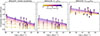 |
Fig. 4. Clumpiness measured within the larger 200 pc radius aperture, plotted as a function of AGN X-ray luminosity, Panels, lines, and markers are as in Figure 2. |
For LX > 1041.5 erg s−1, local AGNs exhibit an anticorrelation between LX and the molecular gas concentration index, defined as the ratio of surface densities within the 50 pc and 200 pc apertures (see García-Burillo et al. 2024). To compare with these findings, we calculated the ratio of clumpiness estimates within the two apertures for each method and smoothing level. As shown in Figure A.7, with all three methods we observe a rising trend, rather than a flat regime, followed by a decline in the clumpiness ratio as a function of LX, with a break again around 1042 erg s−1. However, substantial scatter is present, likely due to the noise in the larger 200 pc aperture.
4.3. Clumpiness versus concentration
In Figure 5 we explore the relation between the clumpiness measured within the central 50 pc aperture and the cold molecular gas concentration index (CCI ≡log(Σ50/Σ200)). The CCI provides a more global measure of how centrally concentrated the cold molecular gas is, while the clumpiness values in Figure 5 refer to the nuclear region alone.
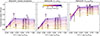 |
Fig. 5. Clumpiness measured within the 50 pc radius aperture, plotted as a function of cold molecular gas concentration index (CCI ≡log(Σ50/Σ200), where Σr is the surface density within an aperture of radius r parsec). Panels, lines, and markers are as in Figure 2. |
With all three methods we observe a rising trend of clumpiness with increasing CCI up to CCI ∼ 0.1, after which the relation flattens. This break point value is significantly lower than the one reported by García-Burillo et al. (2024) in the CCI–LX relation, where the transition occurs around CCI ∼ 0.5.
In Figure A.8 we present the plot of the clumpiness ratio (measured within 50 pc divided by that within 200 pc) as a function of the CCI. In this case all three methods reveal significant correlations, with a clear break at CCI ∼ 0.6. This break point is closer to the value found by García-Burillo et al. (2024) in the CCI–LX relation.
5. Discussion
5.1. Comparison with previous studies
Method #1 allows us to compare our measured clumpiness values with existing literature, as it is the same method originally developed by Conselice (2003). In their work median clumpiness, measured from stellar light in the optical R band, ranges from 0 for elliptical galaxies to ∼0.7 for starburst galaxies, with data smoothed using a kernel of size 0.3 × R(η = 0.2), where R(η) is the Petrosian radius2. Yamamoto et al. (2025) found a median clumpiness of 0.27 ± 0.08 from ALMA CO(2 − 1) maps in a PHANGS subsample, mostly composed of spiral galaxies. Their ALMA data, at 180 pc resolution, were smoothed with a kernel of size 0.3 × Re, where the effective radius Re of the galaxy was chosen instead of R(η = 0.2) to better represent the spatial extent of CO(2 − 1). For example, for the PHANGS galaxy NGC 3627, Re ≈ 66″, whereas R(η = 0.2)≈178″ (3.6 and 9.7 kpc, respectively).
In our case, using Method #1, we find the median clumpiness in the nuclear 50 pc aperture to range from  to
to  (with the upper and lower values representing the 1σ deviation of the sample), depending on the smoothing kernel size (20 − 100 pc; see Figure 2). In the larger 200 pc aperture, these values become
  and
and  , respectively, for 20 pc and 100 pc smoothing (see Figure 4).
At first these results may suggest that the molecular gas clumpiness in the nuclear regions of AGN-host galaxies is comparable to that observed in the disks of normal spirals (PHANGS) and significantly lower than the values found for the stellar emission of starburst galaxies. However, a direct comparison is not straightforward because the measured clumpiness depends critically on the spatial scale traced by the data and on the chosen smoothing kernel. In our case we probe only the central few hundred parsecs at a much higher resolution (16 pc), and by applying different smoothing kernels (from 20 to 100 pc) we can highlight structures of different physical sizes. In contrast the study by Yamamoto et al. (2025) covers entire galaxy disks with lower resolution (180 pc), and their smoothing kernel is several kiloparsecs, making it more sensitive to large-scale molecular complexes.
5.2. Clumpiness as a function of X-ray luminosity
By exploring clumpiness as a function of smoothing scale, we find distinct behaviors depending on the method adopted. With Methods #1 and #2, small-scale structures (highlighted by smoothing kernels ≲50 pc) show generally low clumpiness values and an anticorrelation with AGN luminosity. At larger smoothing scales (≳80 pc), clumpiness remains roughly constant with AGN luminosity up to LX ≈ 1042 erg s−1, followed by a clear drop at higher luminosities. This behavior may suggest that larger molecular structures (∼80 − 100 pc) are more resilient to moderate AGN feedback (as traced by LX) but are eventually disrupted when the AGN becomes sufficiently powerful.
In contrast, Method #3 consistently reveals a statistically significant break point around LX ≈ 1042 erg s−1, even at the smallest scales (∼30 pc). This indicates that, regardless of the physical scale probed, the fraction of emission associated with compact clumps decreases sharply once the AGN reaches high luminosities. Such behavior supports the idea that AGN activity can impact both small (≲50 pc) and large (≳80 pc) molecular structures, potentially through a combination of X-ray irradiation, winds, and cosmic rays.
The different emergence of the break point between Methods #2 and #3 likely reflects the stronger sensitivity of Method #2 to the contrast between clumps and background. At small smoothing scales, more luminous AGNs seem to reduce this contrast, leading to lower values of ΣI − B. Method #3, which does not subtract the background, is less affected and therefore reveals the break point already at small scales. At larger smoothing (≥60 pc), the background level decreases and the contrast naturally diminishes, causing the two methods to converge.
The observed flat regime followed by a decline in clumpiness at LX ≈ 1042 erg s−1 could be the result of a balance between significant gas inflow from the outer regions (driven by gravitational torque; see, e.g., García-Burillo et al. 2005; Casasola et al. 2008; Combes et al. 2014; Querejeta et al. 2016b; Audibert et al. 2019, 2021) and the mild AGN feedback acting on molecular gas in galaxies below the luminosity break point. In this scenario the nuclear regions (within 50 pc from the AGN) maintain their clumpiness up to a certain AGN luminosity thanks to the continuous feeding of fresh molecular material, until the feedback becomes strong enough to dominate and disperse the larger molecular complexes.
We note that the three methods we developed to quantify clumpiness, despite being sensitive to different systematics, consistently reveal the same negative trend with LX. This agreement strengthens the robustness of our finding that higher AGN luminosity is associated with smoother gas distributions.
Interestingly, when measuring clumpiness in the larger aperture (200 pc radius, Figure 4), we do not observe the same turnover. Instead, we find a continuous anticorrelation with AGN luminosity, independently of the smoothing kernel size. This may be because, in the larger aperture, we lose the direct view of the nuclear clumpiness and instead average over a broader region of the circumnuclear disk. In this larger region, the inflow of molecular gas at low LX may be not sufficient to balance the AGN feedback at any of the smoothing scales considered, resulting in a continuous anticorrelation between clumpiness and AGN luminosity. It is also worth noting that, in this larger aperture, the results for some galaxies may be affected by higher noise levels, which can bias the clumpiness measurement. Furthermore, when we isolate the annular region between 50 and 200 pc to exclude the nucleus, the anticorrelation with AGN luminosity nearly disappears (see Figure A.6), suggesting that the observed trend is mostly driven by the nuclear region itself.
The clumpiness measured in the central 50 pc could in principle reflect the efficiency of AGN feeding. Our analysis indeed shows a significant correlation (especially with Methods #1 and #3) with the AGN Eddington ratio λEdd (Figure A.5). This may suggest that the small-scale molecular gas structure is impacted not only by the AGN radiative power traced by LX, that is, by the number of high-energy photons, but also by the shape of the spectral energy distribution and/or the black hole mass, both of which influence λEdd.
5.3. Clumpiness as a function of gas concentration
Our analysis of the molecular gas clumpiness within the central 50 pc shows complex behavior when compared to the cold molecular gas concentration index (CCI), which quantifies the radial concentration of molecular gas between 50 and 200 pc scales (see Figure 5). At any smoothing scale, clumpiness seems to be correlated with CCI, with a break point around CCI ∼ 0.1. The absence of a one-to-one correlation implies that other hidden variables, likely including AGN luminosity and feedback processes, also influence gas morphology. Notably, in the clumpiness ratio versus CCI plot presented in Figure A.8, a similar correlation emerges with a break point around CCI ∼ 0.6, close to the break found in the CCI versus LX plot by García-Burillo et al. (2024).
We note that a correlation between clumpiness and concentration was also reported by Conselice (2003) for stellar light emission on kiloparsec scales: in their case clumpiness correlated with Hα emission from young stars, while concentration was linked to the bulge-to-total light ratio. In our study these quantities are measured from molecular gas emission within the nuclear 400 pc. Nonetheless, the observed structural change in the molecular gas – from a clumpier to a smoother distribution with increasing AGN luminosity – may have important implications for the host galaxy. A smoother gas distribution could indicate the suppression of dense molecular clouds, thereby reducing the local star formation rate, and at the same time make the gas more vulnerable to being entrained and expelled by AGN-driven winds (see, e.g., Ward et al. 2024). On the other hand, at lower LX, the higher degree of clumpiness may negatively affect the propagation of jets and winds, causing them to scatter and dissipate their kinetic energy more efficiently into the surrounding ISM (Perucho & Bosch-Ramon 2012; Wagner et al. 2012; Mukherjee et al. 2018; Tanner & Weaver 2022).
6. Conclusions
In this study we investigated several methods for measuring the clumpiness of the cold molecular gas in the nuclear region (50 − 200 pc) of galaxies. We examined its relationship with AGN activity, as measured by the X-ray 2 − 10 keV luminosity LX, as well as with cold molecular gas concentration, measured by the index CCI ≡log(Σ50/Σ200).
By analyzing how clumpiness changes with smoothing scale, we find that small-scale molecular structures (revealed by smoothing ≲ 50 pc) generally exhibit lower clumpiness values and an anticorrelation with AGN luminosity across the entire range of LX considered (see Figure 2). In contrast, when probing larger molecular structures (∼70 − 100 pc) – or when estimating clumpiness more directly, by summing over the clumps without subtracting the underlying background emission – we observe a different behavior: clumpiness remains roughly constant up to a threshold luminosity of LX ≈ 1042 erg s−1, beyond which it drops sharply (see Figure 3). This suggests that larger gas clumps may resist AGN feedback at moderate luminosities, possibly due to the ongoing inflow that replenishes the nuclear region, but are eventually disrupted at higher AGN power. When measuring clumpiness in the larger 400 pc aperture, however, this turnover effect is not observed: we instead find a continuous anticorrelation with LX. We also find evidence for a correlation between clumpiness and concentration (CCI), particularly at low CCI values (CCI < 0), while at higher CCI the relation becomes weaker and consistent with a plateau (see Figure 5).
Our interpretation is that AGN feedback partially destroys nuclear molecular gas (hence decreasing its concentration; García-Burillo et al. 2021, 2024) and smooths the surviving clouds, resulting in a less clumpy medium. We interpret this as evidence of negative AGN feedback in the immediate surroundings of the AGN, where the gas becomes less capable of aggregating into dense clouds – a necessary condition for star formation.
It is worth noting that these results were made possible by the high spatial resolution (16 pc) of the gas observations, which allowed us to probe the molecular gas in unprecedented detail. In contrast, hydrodynamical simulations still face challenges in capturing the full complexity of the molecular ISM, particularly in modeling the interaction between AGN winds and a clumpy medium, due to the coexistence of vastly different physical scales and gas phases (e.g., McCourt et al. 2018; Meenakshi et al. 2022; Ward et al. 2024).
The results presented here not only reveal a negative correlation between clumpiness and AGN activity, but also highlight the distinct impact of AGN feedback on gas structures at small spatial scales, an aspect that has been poorly investigated in previous studies. As clumpiness becomes an increasingly important parameter for characterizing both nearby (Leroy et al. 2013; Sun et al. 2022; Yamamoto et al. 2025) and distant galaxies (Murata et al. 2014; Sok et al. 2025), our analysis offers a complementary perspective on how AGN activity may shape the internal structure of the molecular gas.
The Petrosian radius is defined as the location where the ratio of surface brightness at a radius, divided by the surface brightness within the radius, reaches a value η (Petrosian 1976).
Acknowledgments
We thank the anonymous referee for suggestions and comments that helped to improve the presentation of this work. We acknowledge the use of Python (Van Rossum & Drake 2009) and the following libraries: Astropy (Astropy Collabration 2013, 2018), Matplotlib (Hunter 2007), NumPy (Harris et al. 2020), Pandas (pandas development team 2020), Photutils (Bradley et al. 2024), pwlf (Jekel & Venter 2019), Seaborn (Waskom 2021), and SciPy (Virtanen et al. 2020). This paper makes use of the following ALMA data: ADS/JAO.ALMA#2015.0.00404.S, #2016.1.00254.S, #2016.0.00296.S, #2017.1.00082.S, and #2018.1.00113.S. ALMA is a partnership of ESO (representing its member states), NSF (USA) and NINS (Japan), together with NRC (Canada), MOST and ASIAA (Taiwan), and KASI (Republic of Korea), in cooperation with the Republic of Chile. The Joint ALMA Observatory is operated by ESO, AUI/NRAO and NAOJ. This research has made use of the NASA/IPAC Extragalactic Database (NED), which is funded by the National Aeronautics and Space Administration and operated by the California Institute of Technology. FE acknowledges support from ESA through the Science Faculty – Funding reference ESA-SCI-E-LE-092. FE, SGB, MQ, and AU acknowledge support from the Spanish grant PID2022-138560NB-I00, funded by MCIN/AEI/10.13039/501100011033/FEDER, EU. AAH acknowledges support from grant PID2021-124665NB-I00 funded by MCIN/AEI/10.13039/501100011033 and by ERDF A way of making Europe. AA acknowledges funding from the European Union grant WIDERA ExGal-Twin, GA 101158446. AJB acknowledges funding from the “FirstGalaxies” Advanced Grant from the European Research Council (ERC) under the European Union’s Horizon 2020 research and innovation program (Grant agreement No. 789056). CRA and AA acknowledge support from project “Tracking active galactic nuclei feedback from parsec to kiloparsec scales”, with reference PID2022-141105NB-I00. EB acknowledges support from the Spanish grants PID2022-138621NB-I00 and PID2021-123417OB-I00, funded by MCIN/AEI/10.13039/501100011033/FEDER, EU. IGB is supported by the Programa Atraccíon de Talento Investigador “César Nombela” via grant 2023-T1/TEC-29030 funded by the Community of Madrid. OGM acknowledge financial support for PAPIIT/UNAM project IN1097123 and Ciencia de Frontera (SECIHTI) project CF-2023-G100. SFH acknowledges support through UK Research and Innovation (UKRI) under the UK government’s Horizon Europe funding Guarantee (EP/Z533920/1) and an STFC Small Award (ST/Y001656/1).
References
- Alonso-Herrero, A., García-Burillo, S., Hönig, S. F., et al. 2021, A&A, 652, A99 [NASA ADS] [CrossRef] [EDP Sciences] [Google Scholar]
- Astropy Collabration (Robitaille, T. P., et al.) 2013, A&A, 558, A33 [NASA ADS] [CrossRef] [EDP Sciences] [Google Scholar]
- Astropy Collabration (Price-Whelan, A. M., et al.) 2018, AJ, 156, 123 [Google Scholar]
- Audibert, A., Combes, F., García-Burillo, S., et al. 2019, A&A, 632, A33 [NASA ADS] [CrossRef] [EDP Sciences] [Google Scholar]
- Audibert, A., Combes, F., García-Burillo, S., et al. 2021, A&A, 656, A60 [NASA ADS] [CrossRef] [EDP Sciences] [Google Scholar]
- Baumgartner, W. H., Tueller, J., Markwardt, C. B., et al. 2013, ApJS, 207, 19 [Google Scholar]
- Bergin, E. A., & Tafalla, M. 2007, ARA&A, 45, 339 [Google Scholar]
- Bertola, E., Circosta, C., Ginolfi, M., et al. 2024, A&A, 691, A178 [NASA ADS] [CrossRef] [EDP Sciences] [Google Scholar]
- Bessiere, P. S., & Ramos Almeida, C. 2022, MNRAS, 512, L54 [NASA ADS] [CrossRef] [Google Scholar]
- Bischetti, M., Maiolino, R., Carniani, S., et al. 2019, A&A, 630, A59 [NASA ADS] [CrossRef] [EDP Sciences] [Google Scholar]
- Bolatto, A. D., Wolfire, M., & Leroy, A. K. 2013, ARA&A, 51, 207 [CrossRef] [Google Scholar]
- Bradley, L., Sipőcz, B., Robitaille, T., et al. 2024, https://doi.org/10.5281/zenodo.13989456 [Google Scholar]
- Buck, T., Pfrommer, C., Girichidis, P., & Corobean, B. 2022, MNRAS, 513, 1414 [NASA ADS] [CrossRef] [Google Scholar]
- Carniani, S., Marconi, A., Maiolino, R., et al. 2017, A&A, 605, A105 [NASA ADS] [CrossRef] [EDP Sciences] [Google Scholar]
- Casasola, V., Combes, F., García-Burillo, S., et al. 2008, A&A, 490, 61 [NASA ADS] [CrossRef] [EDP Sciences] [Google Scholar]
- Chevance, M., Kruijssen, J. M. D., Vazquez-Semadeni, E., et al. 2020, Space Sci. Rev., 216, 50 [NASA ADS] [CrossRef] [Google Scholar]
- Chevance, M., Krumholz, M. R., McLeod, A. F., et al. 2023, ASP Conf. Ser., 534, 1 [NASA ADS] [Google Scholar]
- Cicone, C., Maiolino, R., Sturm, E., et al. 2014, A&A, 562, A21 [NASA ADS] [CrossRef] [EDP Sciences] [Google Scholar]
- Circosta, C., Mainieri, V., Lamperti, I., et al. 2021, A&A, 646, A96 [EDP Sciences] [Google Scholar]
- Combes, F., García-Burillo, S., Casasola, V., et al. 2014, A&A, 565, A97 [NASA ADS] [CrossRef] [EDP Sciences] [Google Scholar]
- Combes, F., García-Burillo, S., Audibert, A., et al. 2019, A&A, 623, A79 [NASA ADS] [CrossRef] [EDP Sciences] [Google Scholar]
- Conselice, C. J. 2003, ApJS, 147, 1 [NASA ADS] [CrossRef] [Google Scholar]
- Crutcher, R. M. 2012, ARA&A, 50, 29 [Google Scholar]
- Elia, D., Strafella, F., Dib, S., et al. 2018, MNRAS, 481, 509 [Google Scholar]
- Ellison, S. L., Wong, T., Sánchez, S. F., et al. 2021, MNRAS, 505, L46 [NASA ADS] [CrossRef] [Google Scholar]
- Elmegreen, B. G., & Falgarone, E. 1996, ApJ, 471, 816 [NASA ADS] [CrossRef] [Google Scholar]
- Esposito, F., Vallini, L., Pozzi, F., et al. 2022, MNRAS, 512, 686 [NASA ADS] [CrossRef] [Google Scholar]
- Esposito, F., Vallini, L., Pozzi, F., et al. 2024a, MNRAS, 527, 8727 [Google Scholar]
- Esposito, F., Alonso-Herrero, A., García-Burillo, S., et al. 2024b, A&A, 686, A46 [NASA ADS] [CrossRef] [EDP Sciences] [Google Scholar]
- Fabian, A. C. 2012, ARA&A, 50, 455 [Google Scholar]
- Faucher-Giguère, C.-A., & Quataert, E. 2012, MNRAS, 425, 605 [Google Scholar]
- Federrath, C., & Klessen, R. S. 2012, ApJ, 761, 156 [Google Scholar]
- Fiore, F., Feruglio, C., Shankar, F., et al. 2017, A&A, 601, A143 [NASA ADS] [CrossRef] [EDP Sciences] [Google Scholar]
- Fluetsch, A., Maiolino, R., Carniani, S., et al. 2019, MNRAS, 483, 4586 [NASA ADS] [Google Scholar]
- Francis, L., Johnstone, D., Herczeg, G., Hunter, T. R., & Harsono, D. 2020, AJ, 160, 270 [NASA ADS] [CrossRef] [Google Scholar]
- Fukui, Y., & Kawamura, A. 2010, ARA&A, 48, 547 [NASA ADS] [CrossRef] [Google Scholar]
- Fuller, L., Lopez-Rodriguez, E., García-Bernete, I., et al. 2025, ApJS, 276, 64 [Google Scholar]
- Gabici, S. 2022, A&ARv, 30, 4 [NASA ADS] [CrossRef] [Google Scholar]
- García, P., Bronfman, L., Nyman, L.-Å., Dame, T. M., & Luna, A. 2014, ApJS, 212, 2 [CrossRef] [Google Scholar]
- García-Bernete, I., Alonso-Herrero, A., García-Burillo, S., et al. 2021, A&A, 645, A21 [EDP Sciences] [Google Scholar]
- García-Bernete, I., Alonso-Herrero, A., Rigopoulou, D., et al. 2024a, A&A, 681, L7 [NASA ADS] [CrossRef] [EDP Sciences] [Google Scholar]
- García-Bernete, I., Rigopoulou, D., Donnan, F. R., et al. 2024b, A&A, 691, A162 [NASA ADS] [CrossRef] [EDP Sciences] [Google Scholar]
- García-Burillo, S., Combes, F., Schinnerer, E., Boone, F., & Hunt, L. K. 2005, A&A, 441, 1011 [NASA ADS] [CrossRef] [EDP Sciences] [Google Scholar]
- García-Burillo, S., Alonso-Herrero, A., Ramos Almeida, C., et al. 2021, A&A, 652, A98 [NASA ADS] [CrossRef] [Google Scholar]
- García-Burillo, S., Hicks, E. K. S., Alonso-Herrero, A., et al. 2024, A&A, 689, A347 [NASA ADS] [CrossRef] [EDP Sciences] [Google Scholar]
- Genzel, R., Förster Schreiber, N. M., Rosario, D., et al. 2014, ApJ, 796, 7 [Google Scholar]
- Harris, C. R., Millman, K. J., van der Walt, S. J., et al. 2020, Nature, 585, 357 [NASA ADS] [CrossRef] [Google Scholar]
- Harrison, C. M., & Ramos Almeida, C. 2024, Galaxies, 12, 17 [NASA ADS] [CrossRef] [Google Scholar]
- Harrison, C. M., Costa, T., Tadhunter, C. N., et al. 2018, Nat. Astron., 2, 198 [Google Scholar]
- Heckman, T. M., & Best, P. N. 2014, ARA&A, 52, 589 [Google Scholar]
- Heyer, M., & Dame, T. M. 2015, ARA&A, 53, 583 [Google Scholar]
- Hunter, J. D. 2007, Comput. Sci. Eng., 9, 90 [NASA ADS] [CrossRef] [Google Scholar]
- Israel, F. P. 2020, A&A, 635, A131 [NASA ADS] [CrossRef] [EDP Sciences] [Google Scholar]
- Jekel, C. F., & Venter, G. 2019, pwlf: A Python Library for Fitting 1D Continuous Piecewise Linear Functions [Google Scholar]
- Kormendy, J., & Ho, L. C. 2013, ARA&A, 51, 511 [Google Scholar]
- Koss, M., Trakhtenbrot, B., Ricci, C., et al. 2017, ApJ, 850, 74 [Google Scholar]
- Koutsoumpou, E., Fernández-Ontiveros, J. A., Dasyra, K. M., & Spinoglio, L. 2025, A&A, 693, A215 [NASA ADS] [CrossRef] [EDP Sciences] [Google Scholar]
- Krajnović, D., Cappellari, M., de Zeeuw, P. T., & Copin, Y. 2006, MNRAS, 366, 787 [Google Scholar]
- Krumholz, M. R. 2014, Phys. Rep., 539, 49 [Google Scholar]
- Krumholz, M. R., McKee, C. F., & Bland-Hawthorn, J. 2019, ARA&A, 57, 227 [NASA ADS] [CrossRef] [Google Scholar]
- Leroy, A. K., Lee, C., Schruba, A., et al. 2013, ApJ, 769, L12 [NASA ADS] [CrossRef] [Google Scholar]
- Leroy, A. K., Schinnerer, E., Hughes, A., et al. 2021, ApJS, 257, 43 [NASA ADS] [CrossRef] [Google Scholar]
- Maiolino, R., Gallerani, S., Neri, R., et al. 2012, MNRAS, 425, L66 [Google Scholar]
- Maiolino, R., Russell, H. R., Fabian, A. C., et al. 2017, Nature, 544, 202 [Google Scholar]
- Maloney, P. R., Hollenbach, D. J., & Tielens, A. G. G. M. 1996, ApJ, 466, 561 [Google Scholar]
- Massi, F., Weiss, A., Elia, D., et al. 2019, A&A, 628, A110 [EDP Sciences] [Google Scholar]
- McCourt, M., Oh, S. P., O’Leary, R., & Madigan, A.-M. 2018, MNRAS, 473, 5407 [Google Scholar]
- McKee, C. F., & Ostriker, E. C. 2007, ARA&A, 45, 565 [Google Scholar]
- Meenakshi, M., Mukherjee, D., Wagner, A. Y., et al. 2022, MNRAS, 516, 766 [NASA ADS] [CrossRef] [Google Scholar]
- Mercedes-Feliz, J., Anglés-Alcázar, D., Hayward, C. C., et al. 2023, MNRAS, 524, 3446 [NASA ADS] [CrossRef] [Google Scholar]
- Mingozzi, M., Vallini, L., Pozzi, F., et al. 2018, MNRAS, 474, 3640 [NASA ADS] [CrossRef] [Google Scholar]
- Morganti, R. 2017, Front. Astron. Space Sci., 4, 42 [CrossRef] [Google Scholar]
- Mukherjee, D., Bicknell, G. V., Wagner, A. Y., Sutherland, R. S., & Silk, J. 2018, MNRAS, 479, 5544 [NASA ADS] [CrossRef] [Google Scholar]
- Murata, K. L., Kajisawa, M., Taniguchi, Y., et al. 2014, ApJ, 786, 15 [NASA ADS] [CrossRef] [Google Scholar]
- Namekata, D., Umemura, M., & Hasegawa, K. 2014, MNRAS, 443, 2018 [Google Scholar]
- Nims, J., Quataert, E., & Faucher-Giguère, C.-A. 2015, MNRAS, 447, 3612 [NASA ADS] [CrossRef] [Google Scholar]
- Omont, A. 2007, Rep. Prog. Phys., 70, 1099 [NASA ADS] [CrossRef] [Google Scholar]
- pandas development team 2020, https://doi.org/10.5281/zenodo.3509134 [Google Scholar]
- Perucho, M., & Bosch-Ramon, V. 2012, A&A, 539, A57 [NASA ADS] [CrossRef] [EDP Sciences] [Google Scholar]
- Petrosian, V. 1976, ApJ, 210, L53 [NASA ADS] [CrossRef] [Google Scholar]
- Pier, E. A., & Voit, G. M. 1995, ApJ, 450, 628 [NASA ADS] [CrossRef] [Google Scholar]
- Poitevineau, R., Combes, F., Garcia-Burillo, S., et al. 2025, A&A, 693, A311 [NASA ADS] [CrossRef] [EDP Sciences] [Google Scholar]
- Pozzi, F., Vallini, L., Vignali, C., et al. 2017, MNRAS, 470, L64 [NASA ADS] [CrossRef] [Google Scholar]
- Querejeta, M., Schinnerer, E., García-Burillo, S., et al. 2016a, A&A, 593, A118 [NASA ADS] [CrossRef] [EDP Sciences] [Google Scholar]
- Querejeta, M., Meidt, S. E., Schinnerer, E., et al. 2016b, A&A, 588, A33 [NASA ADS] [CrossRef] [EDP Sciences] [Google Scholar]
- Ramos Almeida, C., Bischetti, M., García-Burillo, S., et al. 2022, A&A, 658, A155 [NASA ADS] [CrossRef] [EDP Sciences] [Google Scholar]
- Ricci, C., Trakhtenbrot, B., Koss, M. J., et al. 2017, ApJS, 233, 17 [Google Scholar]
- Rosario, D. J., Togi, A., Burtscher, L., et al. 2019, ApJ, 875, L8 [NASA ADS] [CrossRef] [Google Scholar]
- Sabatini, G., Gruppioni, C., Massardi, M., et al. 2018, MNRAS, 476, 5417 [NASA ADS] [CrossRef] [Google Scholar]
- Schartmann, M., Krause, M., & Burkert, A. 2011, MNRAS, 415, 741 [Google Scholar]
- Sok, V., Muzzin, A., Jablonka, P., et al. 2025, ApJ, 979, 14 [Google Scholar]
- Solomon, P. M., Rivolo, A. R., Barrett, J., & Yahil, A. 1987, ApJ, 319, 730 [Google Scholar]
- Sun, J., Leroy, A. K., Rosolowsky, E., et al. 2022, AJ, 164, 43 [NASA ADS] [CrossRef] [Google Scholar]
- Tadaki, K., Esposito, F., Vallini, L., et al. 2025, Nat. Astron., 9, 720 [Google Scholar]
- Tanner, R., & Weaver, K. A. 2022, AJ, 163, 134 [NASA ADS] [CrossRef] [Google Scholar]
- Vallini, L., Ferrara, A., Pallottini, A., & Gallerani, S. 2017, MNRAS, 467, 1300 [NASA ADS] [Google Scholar]
- Van Rossum, G., & Drake, F. L. 2009, Python 3 Reference Manual (Scotts Valley, CA: CreateSpace) [Google Scholar]
- Virtanen, P., Gommers, R., Oliphant, T. E., et al. 2020, Nat. Methods, 17, 261 [Google Scholar]
- Viti, S., García-Burillo, S., Fuente, A., et al. 2014, A&A, 570, A28 [NASA ADS] [CrossRef] [EDP Sciences] [Google Scholar]
- Wagner, A. Y., Bicknell, G. V., & Umemura, M. 2012, ApJ, 757, 136 [CrossRef] [Google Scholar]
- Ward, S. R., Costa, T., Harrison, C. M., & Mainieri, V. 2024, MNRAS, 533, 1733 [Google Scholar]
- Waskom, M. L. 2021, J. Open Source Software, 6, 3021 [NASA ADS] [CrossRef] [Google Scholar]
- Wolfire, M. G., Vallini, L., & Chevance, M. 2022, ARA&A, 60, 247 [NASA ADS] [CrossRef] [Google Scholar]
- Yamamoto, T., Iono, D., Saito, T., et al. 2025, PASJ, 77, 288 [Google Scholar]
- Zhang, L., Packham, C., Hicks, E. K. S., et al. 2024, ApJ, 974, 195 [NASA ADS] [CrossRef] [Google Scholar]
Appendix A: Ancillary material: Sensitivities, emission maps, clumpiness analysis, and additional correlations
In this appendix we present the main ancillary information and visual material used in this study. Table A.1 lists the basic properties of the 16 galaxies analysed: equatorial coordinates, luminosity distances, hard X-ray luminosity (LX), Eddington ratios (λEdd), inclinations, and position angles.
Figure A.1 shows the RMS sensitivity (in Jy km s−1 beam−1) as a function of luminosity distance, demonstrating that there is no correlation between the two. Figure A.2 presents the same sensitivities converted into molecular mass surface densities (M⊙ pc−2), using the conversion factors discussed in Section 2. In addition, we show the ALMA CO(3 − 2) integrated intensity maps (moment 0) of the sample (Figure A.3).
For four representative galaxies, we present the clumpiness maps computed at different smoothing scales (Figure A.4). The galaxies are selected to cover the LX range: NGC 1326 (LX = 1039.9 erg s−1), NGC 6300 (LX = 1041.7 erg s−1), NGC 3227 (LX = 1042.4 erg s−1), and NGC 7582 (LX = 1043.5 erg s−1). These maps illustrate how the choice of smoothing kernel highlights structures of different sizes and contrast in the molecular gas distribution.
We also present additional tests and correlations to complement the main results described in Section 4. Specifically, we explore how clumpiness varies with the Eddington ratio (Figure A.5), when measured in an annular region excluding the nucleus (Figure A.6), and how the ratio of nuclear to circumnuclear clumpiness depends on AGN luminosity and molecular gas concentration (Figures A.7 and A.8).
Properties of the sample.
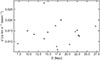 |
Fig. A.1. RMS sensitivities (σ) of the CO(3 − 2) maps in units of Jy kms−1 beam−1 as a function of luminosity distance (in Mpc). No correlation is found between sensitivity and distance. |
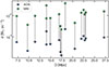 |
Fig. A.2. RMS sensitivities (σ) of the CO(3 − 2) maps converted into molecular mass surface densities (in M⊙ pc−2) as a function of luminosity distance (in Mpc). For each galaxy we show two values, connected by a vertical bar: green squares correspond to the case r31 = 0.7 (average value in galaxy centers, Israel 2020) combined with the standard Milky Way disk conversion factor XCO = 2 × 10²⁰ mol cm−2 (K km s−1)−1 (Bolatto et al. 2013); blue stars correspond to the case r31 = 2.9 (measured at the AGN position in NGC 1068, Viti et al. 2014) combined with the recommended conversion factor for the nuclear region of the Milky Way XCO = 0.5 × 10²⁰ mol cm−2 (K km s−1)−1 (Bolatto et al. 2013). |
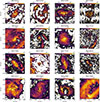 |
Fig. A.3. CO(3 − 2) images of the sample galaxies. Each image covers a region of 400 pc × 400 pc, as in Figure 1. The two ellipses in each panel correspond to circles with radii of 50 and 200 pc projected onto the plane of the galaxy. The galaxies are ordered by increasing 2 − 10 keV luminosity, from top-left to bottom-right. The contours correspond to (3, 5, 10, 20, 30, 50, 100, 200)×σ. The red ellipse inside the white square at the bottom-right corner of each panel represents the ALMA beam. |
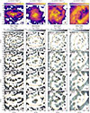 |
Fig. A.4. CO(3 − 2) maps smoothed to a common physical resolution of 16 pc for four representative galaxies (top row): NGC 1326, NGC 6300, NGC 3227, and NGC 7582 (from left to right). The contours are the same as those in Figure A.3. The color bars indicate flux in Jy km s−1 beam−1. From the second to the fifth row, for each galaxy (each column), we show the clumpiness map computed with Method #1 using Gaussian smoothing kernels with a FWHM of 30, 50, 70, and 90 pc (from top to bottom). Contours are plotted every 0.1 between 0 and 1. The two ellipses in each panel correspond to circles with radii of 50 and 200 pc projected onto the plane of the galaxy. The red ellipse inside the white square at the bottom-right corner of each panel represents the ALMA beam. |
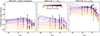 |
Fig. A.5. Clumpiness measured within the 50 pc radius aperture, plotted as a function of the AGN Eddington ratio, λEdd. Panels, lines, and markers are as in Figure 2. |
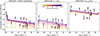 |
Fig. A.6. Clumpiness measured within the annular aperture between 50 and 200 pc, plotted as a function of AGN X-ray luminosity. Panels, lines, and markers are as in Figure 2. |
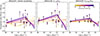 |
Fig. A.7. Ratio of clumpiness measured within the 50 pc radius aperture to that measured within the 200 pc radius aperture, plotted as a function of AGN X-ray luminosity. Panels, lines, and markers are as in Figure 2. |
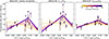 |
Fig. A.8. Ratio of clumpiness measured within the 50 pc radius aperture to that within the 200 pc radius aperture, plotted as a function of the cold molecular gas concentration index, CCI ≡log(Σ50/Σ200). Panels, lines, and markers are as in Figure 2. |
All Tables
All Figures
|
Fig. 1. ALMA observations of the CO(3 − 2) emission in the target galaxy NGC 3227 and the clumpiness computation applied within a 400 pc × 400 pc box around the AGN. First panel: CO(3 − 2) emission at native resolution (10.5 × 9.4 pc), with contours at (3, 5, 10, 20, 30, 50)×σ. Second panel: CO(3 − 2) emission smoothed to a common physical resolution of 16 pc, using contours at the same σ levels. Third panel: CO(3 − 2) emission further smoothed with a Gaussian kernel of FWHM 50 pc, with the same contour levels. Fourth panel: Clumpiness map computed with Method #1 (see Section 3.3), with contours every 0.1 from 0 to 1. In all panels the two ellipses correspond to circles with radii of 50 and 200 pc in the galaxy plane, projected onto the sky. The red ellipse within a square in the bottom right of each panel shows the native ALMA beam (10.5 × 9.4 pc in this case). |
| In the text | |
|
Fig. 2. Clumpiness as a function of AGN intrinsic X-ray 2 − 10 keV luminosity. Clumpiness is measured within the nuclear 50 pc radius aperture with the three different methods described in Section 3.3 (panels left to right). Data points (square markers, nine per galaxy) are colored according to the nine smoothing FWHM sizes adopted (see the color bar in the central panel). The colored lines show the pwlf fits to the data points, with the same color as the fitted dataset; the lines are solid where a linear fit is statistically accepted, and dashed where it is rejected (see Section 3.4). |
| In the text | |
|
Fig. 3. Clumpiness as a function of AGN X-ray luminosity. Clumpiness is measured within the nuclear 50 pc radius aperture with the three different methods described in Section 3.3 (panels left to right). Data points are shown as blue square markers with error bars, computed for a smoothing kernel FWHM of 90 pc. The broken orange lines indicate the pwlf fits to the data, and the shaded regions indicate the corresponding 95% confidence intervals. |
| In the text | |
|
Fig. 4. Clumpiness measured within the larger 200 pc radius aperture, plotted as a function of AGN X-ray luminosity, Panels, lines, and markers are as in Figure 2. |
| In the text | |
|
Fig. 5. Clumpiness measured within the 50 pc radius aperture, plotted as a function of cold molecular gas concentration index (CCI ≡log(Σ50/Σ200), where Σr is the surface density within an aperture of radius r parsec). Panels, lines, and markers are as in Figure 2. |
| In the text | |
|
Fig. A.1. RMS sensitivities (σ) of the CO(3 − 2) maps in units of Jy kms−1 beam−1 as a function of luminosity distance (in Mpc). No correlation is found between sensitivity and distance. |
| In the text | |
|
Fig. A.2. RMS sensitivities (σ) of the CO(3 − 2) maps converted into molecular mass surface densities (in M⊙ pc−2) as a function of luminosity distance (in Mpc). For each galaxy we show two values, connected by a vertical bar: green squares correspond to the case r31 = 0.7 (average value in galaxy centers, Israel 2020) combined with the standard Milky Way disk conversion factor XCO = 2 × 10²⁰ mol cm−2 (K km s−1)−1 (Bolatto et al. 2013); blue stars correspond to the case r31 = 2.9 (measured at the AGN position in NGC 1068, Viti et al. 2014) combined with the recommended conversion factor for the nuclear region of the Milky Way XCO = 0.5 × 10²⁰ mol cm−2 (K km s−1)−1 (Bolatto et al. 2013). |
| In the text | |
|
Fig. A.3. CO(3 − 2) images of the sample galaxies. Each image covers a region of 400 pc × 400 pc, as in Figure 1. The two ellipses in each panel correspond to circles with radii of 50 and 200 pc projected onto the plane of the galaxy. The galaxies are ordered by increasing 2 − 10 keV luminosity, from top-left to bottom-right. The contours correspond to (3, 5, 10, 20, 30, 50, 100, 200)×σ. The red ellipse inside the white square at the bottom-right corner of each panel represents the ALMA beam. |
| In the text | |
|
Fig. A.4. CO(3 − 2) maps smoothed to a common physical resolution of 16 pc for four representative galaxies (top row): NGC 1326, NGC 6300, NGC 3227, and NGC 7582 (from left to right). The contours are the same as those in Figure A.3. The color bars indicate flux in Jy km s−1 beam−1. From the second to the fifth row, for each galaxy (each column), we show the clumpiness map computed with Method #1 using Gaussian smoothing kernels with a FWHM of 30, 50, 70, and 90 pc (from top to bottom). Contours are plotted every 0.1 between 0 and 1. The two ellipses in each panel correspond to circles with radii of 50 and 200 pc projected onto the plane of the galaxy. The red ellipse inside the white square at the bottom-right corner of each panel represents the ALMA beam. |
| In the text | |
|
Fig. A.5. Clumpiness measured within the 50 pc radius aperture, plotted as a function of the AGN Eddington ratio, λEdd. Panels, lines, and markers are as in Figure 2. |
| In the text | |
|
Fig. A.6. Clumpiness measured within the annular aperture between 50 and 200 pc, plotted as a function of AGN X-ray luminosity. Panels, lines, and markers are as in Figure 2. |
| In the text | |
|
Fig. A.7. Ratio of clumpiness measured within the 50 pc radius aperture to that measured within the 200 pc radius aperture, plotted as a function of AGN X-ray luminosity. Panels, lines, and markers are as in Figure 2. |
| In the text | |
|
Fig. A.8. Ratio of clumpiness measured within the 50 pc radius aperture to that within the 200 pc radius aperture, plotted as a function of the cold molecular gas concentration index, CCI ≡log(Σ50/Σ200). Panels, lines, and markers are as in Figure 2. |
| In the text | |
Current usage metrics show cumulative count of Article Views (full-text article views including HTML views, PDF and ePub downloads, according to the available data) and Abstracts Views on Vision4Press platform.
Data correspond to usage on the plateform after 2015. The current usage metrics is available 48-96 hours after online publication and is updated daily on week days.
Initial download of the metrics may take a while.