| Issue |
A&A
Volume 705, January 2026
|
|
|---|---|---|
| Article Number | A177 | |
| Number of page(s) | 20 | |
| Section | Interstellar and circumstellar matter | |
| DOI | https://doi.org/10.1051/0004-6361/202556491 | |
| Published online | 23 January 2026 | |
Variance of dust temperature and spectral index in Planck polarization data using spin-moment expansion
1
Institut d’Astrophysique Spatiale, CNRS, Univ. Paris-Sud, Université Paris-Saclay,
Bât. 121,
91405
Orsay cedex,
France
2
Laboratoire Univers et Particules de Montpellier, Université de Montpellier, CNRS/IN2P2,
CC 72, Place Eugène Bataillon,
34095
Montpellier Cedex 5,
France
3
International School for Advanced Studies (SISSA),
Via Bonomea 265,
34136
Trieste,
Italy
4
Istituto Nazionale di Fisica Nucleare (INFN), Sezione di Trieste,
via Valerio 2,
34127
Trieste,
Italy
5
Institute for Fundamental Physics of the Universe (IFPU),
Via Beirut, 2,
34151
Grignano, Trieste,
Italy
6
IRAP, Université de Toulouse, CNRS, CNES, UPS,
Toulouse,
France
7
Laboratoire de Physique de l’Ecole Normale Supérieure, ENS, Université PSL, CNRS, Sorbonne Université, Université de Paris,
75005
Paris,
France
8
Univ. Grenoble Alpes, CNRS, Grenoble INP, LPSC-IN2P3,
53, avenue des Martyrs,
38000
Grenoble,
France
9
INAF – Osservatorio Astronomico di Cagliari,
Via della Scienza 5,
09047
Selargius,
Italy
10
Laboratoire d’Océanographie Physique et Spatiale (LOPS), Univ. Brest, CNRS, Ifremer, IRD,
29200
Brest,
France
11
INAF – Osservatorio Astrofisico di Arcetri,
Largo E. Fermi 5,
50125
Firenze,
Italy
★ Corresponding author: This email address is being protected from spambots. You need JavaScript enabled to view it.
Received:
18
July
2025
Accepted:
19
October
2025
Abstract
Thermal dust is the major polarized foreground hindering the detection of primordial cosmic microwave background (CMB) B-modes. Its signal exhibits complex behavior in frequency space, arising from the combined variation in our Galaxy of the orientation of magnetic fields and the spectral properties of dust grains aligned with magnetic field lines. In this work, we present a new framework for analyzing the thermal dust signal using polarized microwave data. We introduce residual maps, represented as complex quantities, which capture deviations of the local polarized spectral energy distribution (SED) from the mean complex SED averaged over the sky mask. We present simple predictions that relate the values of the statistical correlation and covariances between the residual maps to the physical properties of the emitting aligned grains. Testing these predictions provides valuable information about the nature of the dust signal. We evaluated our predictions using Planck data over a 97% mask excluding the inner Galactic plane. Despite its simplicity, our model captures a significant part of the statistical properties of the data. For the SRoll2 version of the data, the spectral dependence of the covariances between residual maps is compatible with a dust model that includes only temperature variations rather than spectral index variations. In contrast, for the PR4 Planck official release, it is incompatible with both models. Our methodology can be used to analyze future high-precision polarization data and to build more accurate dust models for use by the CMB community.
Key words: dust, extinction / ISM: magnetic fields / cosmic background radiation
© The Authors 2026
 Open Access article, published by EDP Sciences, under the terms of the Creative Commons Attribution License (https://creativecommons.org/licenses/by/4.0), which permits unrestricted use, distribution, and reproduction in any medium, provided the original work is properly cited.
This article is published in open access under the Subscribe to Open model. This email address is being protected from spambots. You need JavaScript enabled to view it. to support open access publication.
1 Introduction
Observations from the visible to the submillimeter wavelengths (submm) provide extensive evidence on the variations in dust composition and optical properties through the Galaxy. The importance of dust processing in the interstellar medium (ISM) is demonstrated first by the large variations seen in the extinction curve and the depletions of refractory elements (Draine 2003; Jenkins 2009; Schlafly et al. 2016). Additional evidence comes from variations in the spectral energy distribution (SED) and the far-infrared and submm dust opacity of molecular clouds and the diffuse ISM, observed by the Herschel (Ysard et al. 2013) and Planck space missions (Planck Collaboration 2013 XI 2014; Planck Collaboration Int. XVII 2014). These variations of the dust SED include, but are not fully explained by, the dependence of dust temperature on the local intensity of the interstellar radiation field (Fanciullo et al. 2015).
The observational signatures of dust evolution in the dust SED in polarization are harder to identify due to the reduced amplitude of the signal compared to the total intensity (Pelgrims et al. 2021; Ritacco et al. 2023). The interpretation of polarization data considers the combined variations in the structure of the Galactic magnetic field and the dust SED, both in the plane of the sky and along the line of sight in the three-dimensional Galaxy (Tassis & Pavlidou 2015; Planck Collaboration Int. L 2017; McBride et al. 2023; Vacher et al. 2025). This is the specific problem that our work addresses. We present a modeling framework that incorporates variations in dust properties within a turbulent magnetic field, designed to quantify the variance in dust spectral properties from submm polarization data.
In submm polarization maps, the diffuse polarized emission from dust grains that are locally aligned with magnetic-field orientation is summed over the light cone, a small region of the sky observed by the instrumental beam containing both plane-of-the-sky and line-of-sight variations. Variations in the magnetic field orientation within the light cone lead to depolarization (Planck Collaboration Int. XLIV 2016; Clark & Hensley 2019), and their combined variations with changes in dust properties lead to the frequency-dependence of the polarization angle (Tassis & Pavlidou 2015; Planck Collaboration Int. L 2017; Vacher et al. 2023b). For studies of the cosmic microwave background (CMB) polarization, the variation over the sky of dust spectral parameters, and the non-linear distortion they induce in the SEDs, together with their impact on the frequency dependence of polarization angles, makes the separation of the dust and CMB signals a difficult task, especially given the high sensitivity of next-generation experiments (Remazeilles et al. 2016; LiteBIRD Collaboration 2022; Wolz et al. 2024). The modeling of spatial variations in the dust polarization SED is therefore of prime importance for the search for primordial B-modes from inflation and for the putative EB correlation from cosmic birefringence (Diego-Palazuelos et al. 2022, 2023; Vacher et al. 2023a; Jost et al. 2023; Sullivan et al. 2025).
Planck observations show that the mean SED of dust polarized emission in the high-latitude diffuse ISM is remarkably well fitted by a modified black body (MBB) law from 353 GHz to microwave frequencies (Planck Collaboration 2018 XI 2020). This observational result leads us to model spatial variations of the dust polarization SED using the moment expansion method around an MBB, as introduced by Chluba et al. (2017). Previous studies carried out in preparation for future experiments, such as the Simons Observatory and LiteBIRD, show that when spatial variations are present in the foreground SED, the moment-expansion formalism provides a powerful tool to recover the CMB signal without bias, and with minimal parameter addition (Azzoni et al. 2021; Remazeilles et al. 2021; Désert 2022; Vacher et al. 2022; Sponseller & Kogut 2022; Azzoni et al. 2023; Wolz et al. 2024; Carones & Remazeilles 2024). The moment expansion formalism can be extended to polarized dust emission using complex spin-2 fields, referred to as"spin-moment" coefficients (Vacher et al. 2023b,a). In this work, we use this formalism to introduce a modeling framework that, within some simplifying assumptions, accounts for the combined variations of dust properties and magnetic field structure. Applying it to Planck data, we demonstrate the relevance of this framework for analyzing dust polarization microwave observations for foreground modeling and component separation.
Our paper is structured as follows. In Sect. 2, we introduce the dust model and data modeling framework based on complex residual maps. We enumerate the predictions of our model in Sect. 3. In Sect. 4, building on the work of Ritacco et al. (2023), we test the validity of our simplifying assumptions in relation to sky observations by analyzing the Planck SRoll2 maps (Delouis et al. 2019). In Sect. 5, we interpret our results in terms of fluctuations in dust spectral properties and compare them with those obtained using the PR4 version of the Planck data (Planck Collaboration Int. LVII 2020). In Section 6, we discuss our results, which we then summarize in Sect. 7.
2 Model definition
Our dust model and methodology, based on complex numbers, are designed to quantify the variance in the emission properties of grains aligned with magnetic field lines1 which emit polarized radiation in the far-infrared and submm. In Sect. 2.1, we set out the assumptions of our dust signal model and in Sect. 2.2 we show how these hypotheses enable accurate modeling of the polarized signal using complex numbers and the moment expansion. In Sect. 2.5, we define the so-called polarization residual maps, from which we derive various covariances in Sect. 2.6. These covariances are then used to build the predictions of our model in Sect. 3.
2.1 Dust model hypothesis
Our dust model relies on simplifying hypotheses of two kinds: astrophysical (HA) and methodological (HM), listed below.
HA1: the local dust polarized SED emitted at any given position in the Galaxy is a single MBB with local temperature T and local spectral index β.
HA2: the variations of the dust polarization spectral parameters T or β, from one point of the Galaxy to another, are not correlated with variations in the orientation of the magnetic field.
HM3: only two extreme cases are explored: the fluctuations of dust properties are either pure β fluctuations over the whole sky or pure T fluctuations.
HA4: the grain alignment efficiency is uniform over the sky; only the structure of the magnetic field controls the dust polarization fraction. This hypothesis was shown by Planck Collaboration 2018 XII (2020) to be justified at the scale of a degree or more.
HM5: following Planck Collaboration Int. XLVIII (2016), we modeled the structure of magnetic fields as a turbulent field close to equipartition between its ordered and random components.
HM6: our data analysis methodology accounts for contamination of the dust polarization signal in Planck data by CMB, noise, and systematics, but it neglects possible contribution from polarized CO emission or leakage of CO emission in the 217 and 100 GHz channels, as well as the presence of residual synchrotron emission after template removal.
While these hypotheses are quite restrictive, our model is able to generate a frequency-dependence of polarization angles. The simplicity of the model and the clarity of its building hypotheses allow one to infer its predictions unambiguously and to identify its limits precisely. To assist the reader with the numerous notations, Table A.1 summarizes all the quantities used in our model.
2.2 Spin-moment expansion of the complex polarized SED
Following the work of Ritacco et al. (2023), we developed an analytical framework to model the observed variations with the frequency of polarization intensity and angle. For this purpose, we did not use the E and B decomposition (Zaldarriaga & Seljak 1997). Instead, we quantified the total variance of the Stokes parameters. For a given frequency ν, we define the dust complex polarized SED Pν from the Stokes parameters Qν and Uν as follows (complex quantities are written in bold font):
![Mathematical equation: $\[\mathbf{P}_\nu \equiv Q_\nu+\dot{\mathbb{i}} U_\nu=P_\nu \mathrm{e}^{\dot{\mathbb{i}} 2 \psi_\nu},\]$](/articles/aa/full_html/2026/01/aa56491-25/aa56491-25-eq1.png) (1)
(1)
where ![Mathematical equation: $\[\dot{\mathbb{i}}\]$](/articles/aa/full_html/2026/01/aa56491-25/aa56491-25-eq2.png) is the imaginary unit
is the imaginary unit ![Mathematical equation: $\[\left(\dot{\mathbb{i}}^{2}=-1\right), P_{\nu}\]$](/articles/aa/full_html/2026/01/aa56491-25/aa56491-25-eq3.png) is the polarized intensity (
is the polarized intensity (![Mathematical equation: $\[P_{\nu}=\sqrt{Q_{\nu}^{2}+U_{\nu}^{2}}=\sqrt{\mathbf{P}_{\nu} \mathbf{P}_{\nu}^{\star}}\]$](/articles/aa/full_html/2026/01/aa56491-25/aa56491-25-eq4.png) , with ⋆ denoting complex conjugation), and ψν = 0.5 arctan(Uν, Qν) is the frequency-dependent polarization angle.
, with ⋆ denoting complex conjugation), and ψν = 0.5 arctan(Uν, Qν) is the frequency-dependent polarization angle.
Following Vacher et al. (2023b), we note that the use of complex spin-moments is well suited to studying fluctuations in the dust complex polarized SED. The SED Pν observed over a region of the sky is given by the integral over all the local elementary SEDs dPν present within the observed light cone ℒ:
![Mathematical equation: $\[\mathbf{P}_\nu=\int_{\mathcal{L}} \mathrm{d} \mathbf{P}_\nu.\]$](/articles/aa/full_html/2026/01/aa56491-25/aa56491-25-eq5.png) (2)
(2)
Variations in phases in this integral can partially or fully cancel the polarization signal, a phenomenon known as depolarization (Planck Collaboration Int. XIX 2015). The so-called light cone, ℒ, is a region of the sky over which all local signals dPν – contained both in the plane of the sky and along the line of sight – are averaged. Depending on the context of the analysis, ℒ can refer to a map pixel, the instrumental beam, or even the entire sky, possibly masked. In the present work, we considered ℒ to be the instrumental beam surrounding each pixel of the sky.
We used an MBB model of dust emission (hypothesis HA1, Sect. 2.1) characterized by a local spectral index β and a local temperature T to express the local dust emissivity εν(T, β) at frequency ν,
![Mathematical equation: $\[\varepsilon_\nu(\beta, T)=B_\nu(T)\left(\frac{\nu}{\nu_0}\right)^\beta,\]$](/articles/aa/full_html/2026/01/aa56491-25/aa56491-25-eq6.png) (3)
(3)
where Bν(T) is Planck’s law at frequency ν and temperature T, and ν0 is a reference frequency. Assuming that the local complex polarized intensity, dPν0, at frequency ν0 is well-defined in amplitude and phase everywhere in the light cone, the frequency-dependence of the local complex polarized SED, dPν, is
![Mathematical equation: $\[\mathrm{d} \mathbf{P}_\nu=\mathrm{d} \mathbf{P}_{\nu_0} \frac{\varepsilon_\nu(\beta, T)}{\varepsilon_{\nu_0}(\beta, T)}=\mathrm{d} \mathbf{P}_{\nu_0} \frac{B_\nu(T)}{B_{\nu_0}(T)}\left(\frac{\nu}{\nu_0}\right)^\beta.\]$](/articles/aa/full_html/2026/01/aa56491-25/aa56491-25-eq7.png) (4)
(4)
Because the emissivity εν is a real quantity, dPν has the same polarization angle at all frequencies.
To estimate the impact of fluctuations in the spectral parameter s ∈ {T, β} on the observed complex polarized intensity Pν (under our hypothesis HM3, which assumes that either T or β fluctuates over the whole sky but not both), we performed a Taylor expansion of the power-law term and the blackbody in dPν in Eq. (4) around an arbitrary pivot spectral index ![Mathematical equation: $\[\overline{\beta}\]$](/articles/aa/full_html/2026/01/aa56491-25/aa56491-25-eq8.png) and pivot temperature
and pivot temperature ![Mathematical equation: $\[\overline{T}\]$](/articles/aa/full_html/2026/01/aa56491-25/aa56491-25-eq9.png) . We find that the frequency dependence of the complex polarized intensity can be expressed as (Vacher et al. 2023b)
. We find that the frequency dependence of the complex polarized intensity can be expressed as (Vacher et al. 2023b)
![Mathematical equation: $\[\mathbf{P}_\nu=\mathbf{P}_{\nu_0} \frac{\overline{\varepsilon}_\nu}{\overline{\varepsilon}_{\nu_0}}\left(1+{\sum}_{n=1}^{\infty} a_{\nu, n}^s \boldsymbol{\mathcal{W}}_n^s\right),\]$](/articles/aa/full_html/2026/01/aa56491-25/aa56491-25-eq10.png) (5)
(5)
where
![Mathematical equation: $\[\overline{\varepsilon}_\nu \equiv \varepsilon_\nu(\overline{\beta}, \overline{T})\]$](/articles/aa/full_html/2026/01/aa56491-25/aa56491-25-eq11.png) (6)
(6)
is the pivot SED, the function ![Mathematical equation: $\[a_{\nu, n}^{s}\]$](/articles/aa/full_html/2026/01/aa56491-25/aa56491-25-eq12.png) of ν denotes the nth order derivative of the dust emissivity with respect to the spectral parameter s,
of ν denotes the nth order derivative of the dust emissivity with respect to the spectral parameter s,
![Mathematical equation: $\[a_{\nu, n}^s \equiv \frac{1}{n!} \frac{\overline{\varepsilon}_{\nu_0}}{\overline{\varepsilon}_\nu} \frac{\partial^n\left(\varepsilon_\nu / \varepsilon_{\nu_0}\right)}{\partial s^n}(\overline{\beta}, \overline{T}),\]$](/articles/aa/full_html/2026/01/aa56491-25/aa56491-25-eq13.png) (7)
(7)
and ![Mathematical equation: $\[\boldsymbol{\mathcal{W}}_{n}^{s}\]$](/articles/aa/full_html/2026/01/aa56491-25/aa56491-25-eq14.png) is the nth order spin-moment of s (Vacher et al. 2023b), given2 by
is the nth order spin-moment of s (Vacher et al. 2023b), given2 by
![Mathematical equation: $\[\boldsymbol{\mathcal{W}}_n^s \equiv \frac{1}{\mathbf{P}_{\nu_0}} \int_{\mathcal{L}}(s-\overline{s})^n \mathrm{~d} \mathbf{P}_{\nu_0}.\]$](/articles/aa/full_html/2026/01/aa56491-25/aa56491-25-eq15.png) (8)
(8)
The spin-moments ![Mathematical equation: $\[\boldsymbol{\mathcal{W}}_{n}^{s}\]$](/articles/aa/full_html/2026/01/aa56491-25/aa56491-25-eq19.png) encode the departure of the spectral dependence of Pν from the pivot SED
encode the departure of the spectral dependence of Pν from the pivot SED ![Mathematical equation: $\[\overline{\varepsilon}_{\nu}\]$](/articles/aa/full_html/2026/01/aa56491-25/aa56491-25-eq20.png) . The pivot spectral parameters
. The pivot spectral parameters ![Mathematical equation: $\[\overline{\beta}\]$](/articles/aa/full_html/2026/01/aa56491-25/aa56491-25-eq21.png) and
and ![Mathematical equation: $\[\overline{T}\]$](/articles/aa/full_html/2026/01/aa56491-25/aa56491-25-eq22.png) are constant over ℒ. For simplicity, we further considered a single pair of pivots for all light cones and hence the whole sky. In this analysis, we used
are constant over ℒ. For simplicity, we further considered a single pair of pivots for all light cones and hence the whole sky. In this analysis, we used ![Mathematical equation: $\[\overline{T} \equiv 20 \mathrm{~K}\]$](/articles/aa/full_html/2026/01/aa56491-25/aa56491-25-eq23.png) . The specific value for
. The specific value for ![Mathematical equation: $\[\overline{\beta}\]$](/articles/aa/full_html/2026/01/aa56491-25/aa56491-25-eq24.png) is not critical, as it does not appear in the data analysis.
is not critical, as it does not appear in the data analysis.
The frequency dependence of ![Mathematical equation: $\[a_{\nu, n}^{T}\]$](/articles/aa/full_html/2026/01/aa56491-25/aa56491-25-eq25.png) and
and ![Mathematical equation: $\[a_{\nu, n}^{\beta}\]$](/articles/aa/full_html/2026/01/aa56491-25/aa56491-25-eq26.png) is presented in Fig. 1 for n = 1, 2, and 3. Their analytical expression for n = 1 is as follows:
is presented in Fig. 1 for n = 1, 2, and 3. Their analytical expression for n = 1 is as follows:
![Mathematical equation: $\[d_{\nu, 1}^\beta \equiv \ln \left(\nu / \nu_0\right),\]$](/articles/aa/full_html/2026/01/aa56491-25/aa56491-25-eq27.png) (9)
(9)
![Mathematical equation: $\[a_{\nu, 1}^T \equiv \frac{h}{k \overline{T}^2}\left[\frac{\nu \mathrm{e}^{h \nu / k \overline{T}}}{\mathrm{e}^{h \nu / k \overline{T}}-1}-\frac{\nu_0 \mathrm{e}^{h \nu_0 / k \overline{T}}}{\mathrm{e}^{h \nu_0 / k \overline{T}}-1}\right].\]$](/articles/aa/full_html/2026/01/aa56491-25/aa56491-25-eq28.png) (10)
(10)
The values of the ![Mathematical equation: $\[a_{\nu, n}^{s}\]$](/articles/aa/full_html/2026/01/aa56491-25/aa56491-25-eq29.png) functions – hereafter referred to as the spectral gradients – are listed explicitly up to n = 5 for both β and T in Chluba et al. (2017).
functions – hereafter referred to as the spectral gradients – are listed explicitly up to n = 5 for both β and T in Chluba et al. (2017).
The polarization-weighted moment ![Mathematical equation: $\[\boldsymbol{\mathcal{W}}_{n}^{s}\]$](/articles/aa/full_html/2026/01/aa56491-25/aa56491-25-eq30.png) is distinct from the intensity-weighted moments
is distinct from the intensity-weighted moments ![Mathematical equation: $\[\omega_{n}^{s}\]$](/articles/aa/full_html/2026/01/aa56491-25/aa56491-25-eq31.png) (Chluba et al. 2017):
(Chluba et al. 2017):
![Mathematical equation: $\[\omega_n^s \equiv \frac{1}{I} \int_{\mathcal{L}}(s-\overline{s})^n \mathrm{~d} I,\]$](/articles/aa/full_html/2026/01/aa56491-25/aa56491-25-eq32.png) (11)
(11)
with s ∈ {T, β} as before. Like ![Mathematical equation: $\[\boldsymbol{\mathcal{W}}_{n}^{s}, \omega_{n}^{s}\]$](/articles/aa/full_html/2026/01/aa56491-25/aa56491-25-eq33.png) characterizes the statistical properties of the spectral parameters s of aligned grains. However,
characterizes the statistical properties of the spectral parameters s of aligned grains. However, ![Mathematical equation: $\[\omega_{n}^{s}\]$](/articles/aa/full_html/2026/01/aa56491-25/aa56491-25-eq34.png) is independent of the structure of the magnetic field, whereas
is independent of the structure of the magnetic field, whereas ![Mathematical equation: $\[\boldsymbol{\mathcal{W}}_{n}^{s}\]$](/articles/aa/full_html/2026/01/aa56491-25/aa56491-25-eq35.png) is not. The difference between these two moments,
is not. The difference between these two moments,
![Mathematical equation: $\[\Delta_n^s \equiv \boldsymbol{\mathcal{W}}_n^s-\omega_n^s,\]$](/articles/aa/full_html/2026/01/aa56491-25/aa56491-25-eq36.png) (12)
(12)
is a complex quantity of interest. In Appendix B, we demonstrate that, under our hypothesis HA2, which assumes no correlation between the fluctuations of dust spectral properties and variations in the magnetic field direction, ![Mathematical equation: $\[\Delta_{n}^{s}\]$](/articles/aa/full_html/2026/01/aa56491-25/aa56491-25-eq37.png) has a statistically zero mean:
has a statistically zero mean: ![Mathematical equation: $\[\left\langle\boldsymbol{\Delta}_{n}^{s}\right\rangle=0\]$](/articles/aa/full_html/2026/01/aa56491-25/aa56491-25-eq38.png) .
.
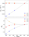 |
Fig. 1 Values of |
![Mathematical equation: $\[a_{\nu}^{\beta}\]$](/articles/aa/full_html/2026/01/aa56491-25/aa56491-25-eq16.png)
![Mathematical equation: $\[a_{\nu}^{T}\]$](/articles/aa/full_html/2026/01/aa56491-25/aa56491-25-eq17.png)
![Mathematical equation: $\[\overline{T}=20 \mathrm{~K}\]$](/articles/aa/full_html/2026/01/aa56491-25/aa56491-25-eq18.png)
2.3 Spectral rotation of polarization angles
To gain further insight into how the spin-moments, ![Mathematical equation: $\[\boldsymbol{\mathcal{W}}_{n}^{s}\]$](/articles/aa/full_html/2026/01/aa56491-25/aa56491-25-eq39.png) , are related to the spectral dependence of Pν, we first consider the specific case of small distortions of the polarized SED around the pivot SED (
, are related to the spectral dependence of Pν, we first consider the specific case of small distortions of the polarized SED around the pivot SED (![Mathematical equation: $\[\left|{\sum}_{n=1}^{\infty} a_{\nu, n}^{s} \boldsymbol{\mathcal{W}}_{n}^{s}\right| \ll 1\]$](/articles/aa/full_html/2026/01/aa56491-25/aa56491-25-eq40.png) ). Taking the logarithm of Eq. (5) and using the approximation ln(1 + x) ~ x for x ≪ 1, we obtain
). Taking the logarithm of Eq. (5) and using the approximation ln(1 + x) ~ x for x ≪ 1, we obtain
![Mathematical equation: $\[\ln \left(\frac{\mathbf{P}_\nu}{\overline{\varepsilon}_\nu}\right)-\ln \left(\frac{\mathbf{P}_{\nu_0}}{\overline{\varepsilon}_{\nu_0}}\right) \simeq {\sum}_{n=1}^{\infty} a_{\nu, n}^s \boldsymbol{\mathcal{W}}_n^s,\]$](/articles/aa/full_html/2026/01/aa56491-25/aa56491-25-eq41.png) (13)
(13)
from which we take the real and imaginary parts and, using Eq. (1),
![Mathematical equation: $\[\ln \left(\frac{P_\nu}{\overline{\varepsilon}_\nu}\right)-\ln \left(\frac{P_{\nu_0}}{\overline{\varepsilon}_{\nu_0}}\right) \simeq {\sum}_{n=1}^{\infty} a_{\nu, n}^s \operatorname{Re} \boldsymbol{\mathcal{W}}_n^s,\]$](/articles/aa/full_html/2026/01/aa56491-25/aa56491-25-eq42.png) (14)
(14)
![Mathematical equation: $\[2\left(\psi_\nu-\psi_{\nu_0}\right) \simeq \sum_{n=1}^{\infty} a_{\nu, n}^s \operatorname{Im} \boldsymbol{\mathcal { W }}_n^s.\]$](/articles/aa/full_html/2026/01/aa56491-25/aa56491-25-eq43.png) (15)
(15)
Equation (15) describes the spectral rotation of the polarization angle with frequency, caused by fluctuations of the dust spectral parameters within the light cone. Its frequency dependence is governed by the ![Mathematical equation: $\[a_{\nu, n}^{s}\]$](/articles/aa/full_html/2026/01/aa56491-25/aa56491-25-eq44.png) parameters and its amplitude depends on the imaginary parts
parameters and its amplitude depends on the imaginary parts ![Mathematical equation: $\[\operatorname{Im \boldsymbol{\mathcal{W}}}_{n}^{s}\]$](/articles/aa/full_html/2026/01/aa56491-25/aa56491-25-eq45.png) of the spin-moments. Figure 2 provides a numerical illustration of such a rotation in the log-complex plane for the sum of seven MBBs with Gaussian-distributed spectral parameters in a turbulent magnetic-field model inspired by Planck Collaboration Int. XLVIII (2016) (see also our description in Appendix C). We consider the two cases of our hypothesis HM3: pure fluctuations in T or pure fluctuations in β. Under the assumption of small variations in T or β, the complex SED plotted in the log-complex plane (ln (Pν/ϵν), 2ψν) is close to a straight line for T fluctuations and can be non-linear for β fluctuations when the magnetic field direction is close to the line of sight (as shown in Fig. 2 for illustration). This shows that, in a given light cone, the rotation of the polarization angle with frequency is strongly correlated with the distortion of the polarized intensity relative to the pivot SED.
of the spin-moments. Figure 2 provides a numerical illustration of such a rotation in the log-complex plane for the sum of seven MBBs with Gaussian-distributed spectral parameters in a turbulent magnetic-field model inspired by Planck Collaboration Int. XLVIII (2016) (see also our description in Appendix C). We consider the two cases of our hypothesis HM3: pure fluctuations in T or pure fluctuations in β. Under the assumption of small variations in T or β, the complex SED plotted in the log-complex plane (ln (Pν/ϵν), 2ψν) is close to a straight line for T fluctuations and can be non-linear for β fluctuations when the magnetic field direction is close to the line of sight (as shown in Fig. 2 for illustration). This shows that, in a given light cone, the rotation of the polarization angle with frequency is strongly correlated with the distortion of the polarized intensity relative to the pivot SED.
2.4 Mean complex normalized SED
From here on, we simplify our notation for channel i of frequency νi and use Pi to denote the map of complex polarized intensity, ![Mathematical equation: $\[\overline{\varepsilon}_{i}\]$](/articles/aa/full_html/2026/01/aa56491-25/aa56491-25-eq46.png) for the pivot emissivity (constant over the sky), and
for the pivot emissivity (constant over the sky), and ![Mathematical equation: $\[a_{i, n}^{s}\]$](/articles/aa/full_html/2026/01/aa56491-25/aa56491-25-eq47.png) for the spectral gradient.
for the spectral gradient.
Following Ritacco et al. (2023), we cross-correlated the polarization maps to determine the mean complex SED ![Mathematical equation: $\[\overline{\mathbf{r}}_{i}\]$](/articles/aa/full_html/2026/01/aa56491-25/aa56491-25-eq48.png) of dust polarization, averaged over the sky and normalized to our reference channel, given by
of dust polarization, averaged over the sky and normalized to our reference channel, given by
![Mathematical equation: $\[\overline{\mathbf{r}}_i \equiv \frac{\left\langle\mathbf{P}_i \mathbf{P}_0^{\star}\right\rangle}{\left\langle\mathbf{P}_0 \mathbf{P}_0^{\star}\right\rangle}=\frac{\overline{\varepsilon}_i}{\overline{\varepsilon}_0}\left(1+{\sum}_{n=1}^{\infty} a_{i, n}^s \overline{\boldsymbol{\mathcal{W}}}_n^s\right),\]$](/articles/aa/full_html/2026/01/aa56491-25/aa56491-25-eq49.png) (16)
(16)
where ![Mathematical equation: $\[\overline{\boldsymbol{\mathcal{W}}}_{n}^{s}\]$](/articles/aa/full_html/2026/01/aa56491-25/aa56491-25-eq50.png) is the mean value of
is the mean value of ![Mathematical equation: $\[\boldsymbol{\mathcal{W}}_{n}^{s}\]$](/articles/aa/full_html/2026/01/aa56491-25/aa56491-25-eq51.png) over the sky, weighted by
over the sky, weighted by ![Mathematical equation: $\[P_{0}^{2}=\mathbf{P}_{0} \mathbf{P}_{0}^{\star}\]$](/articles/aa/full_html/2026/01/aa56491-25/aa56491-25-eq52.png) as
as
![Mathematical equation: $\[\overline{\boldsymbol{\mathcal{W}}}_n^s \equiv\left\langle P_0^2 \boldsymbol{\mathcal{W}}_n^s\right\rangle /\left\langle P_0^2\right\rangle.\]$](/articles/aa/full_html/2026/01/aa56491-25/aa56491-25-eq53.png) (17)
(17)
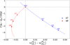 |
Fig. 2 Rotation of the SED in the complex plane for a sum of seven MBB SEDs with distinct spectral indices drawn from a Gaussian distribution with mean 1.5 and standard deviation 0.1 (red), or with temperatures drawn from a Gaussian distribution with mean 20 K and standard deviation 5 K (blue). The 3D orientation of the magnetic field is a random realization of the turbulent magnetic field inspired by Planck Collaboration Int. XLVIII (2016). The dashed lines indicate frequencies from 40 to 400 GHz, and the four colored points represent the Planck HFI bands. |
2.5 Residual maps for complex polarization
In this section, we use the pivot SED to construct complex residual maps at all frequencies and relate them to the ![Mathematical equation: $\[\boldsymbol{\mathcal{W}}_{n}^{s}\]$](/articles/aa/full_html/2026/01/aa56491-25/aa56491-25-eq54.png) moments. We define the residual map Ri for the complex polarization Pi:
moments. We define the residual map Ri for the complex polarization Pi:
![Mathematical equation: $\[\mathbf{R}_i \equiv P_0\left(\frac{1}{\overline{\mathbf{r}}_i} \frac{\mathbf{P}_i}{\mathbf{P}_0}-1\right).\]$](/articles/aa/full_html/2026/01/aa56491-25/aa56491-25-eq55.png) (18)
(18)
This complex map characterizes the residuals at frequency νi after removal of the components correlated with the polarization map at the reference frequency ν0, and subsequently scaled to the reference frequency ν0. Here, Ri quantifies the complexity of the dust signal by measuring its deviations from the mean complex SED ![Mathematical equation: $\[\overline{\mathbf{r}}_{i}\]$](/articles/aa/full_html/2026/01/aa56491-25/aa56491-25-eq56.png) .
.
Using Eqs. (5) and (16), we obtain
![Mathematical equation: $\[\mathbf{R}_i=P_0\left(\frac{1+\sum_{n=1}^{\infty} a_{i, n}^s \boldsymbol{\mathcal{W}}_n^s}{1+\sum_{n=1}^{\infty} a_{i, n}^s \overline{\boldsymbol{\mathcal{W}}}_n^s}-1\right).\]$](/articles/aa/full_html/2026/01/aa56491-25/aa56491-25-eq57.png) (19)
(19)
By choosing the pivot SED close to the mean SED, we ensure that ![Mathematical equation: $\[\left|{\sum}_{n=1}^{\infty} a_{i, n}^{s} \overline{\boldsymbol{\mathcal{W}}}_{n}^{s}\right|=\left|\overline{\mathbf{r}}_{i} \frac{\overline{\varepsilon}_{0}}{\overline{\varepsilon}_{i}}-1\right| \ll 1\]$](/articles/aa/full_html/2026/01/aa56491-25/aa56491-25-eq58.png) (this hypothesis is verified in the data analysis in Sect. 4), so that, by expanding the previous equation to first order, we obtain
(this hypothesis is verified in the data analysis in Sect. 4), so that, by expanding the previous equation to first order, we obtain
![Mathematical equation: $\[\mathbf{R}_i \simeq P_0 {\sum}_{n=1}^{\infty} a_{i, n}^s\left(\boldsymbol{\mathcal{W}}_n^s-\overline{\boldsymbol{\mathcal{W}}}_n^s\right).\]$](/articles/aa/full_html/2026/01/aa56491-25/aa56491-25-eq59.png) (20)
(20)
We decompose Ri into its real and imaginary components:
![Mathematical equation: $\[R_i^P \equiv \operatorname{Re} \mathbf{R}_i=P_0 {\sum}_{n=1}^{\infty} a_{i, n} \operatorname{Re}\left(\boldsymbol{\mathcal{W}}_n^s-\overline{\boldsymbol{\mathcal{W}}}_n^s\right),\]$](/articles/aa/full_html/2026/01/aa56491-25/aa56491-25-eq60.png) (21)
(21)
![Mathematical equation: $\[R_i^\psi \equiv \operatorname{Im} \mathbf{R}_i=P_0 {\sum}_{n=1}^{\infty} a_{i, n} \operatorname{Im}\left(\boldsymbol{\mathcal{W}}_n^s-\overline{\boldsymbol{\mathcal{W}}}_n^s\right).\]$](/articles/aa/full_html/2026/01/aa56491-25/aa56491-25-eq61.png) (22)
(22)
For ![Mathematical equation: $\[R_{i}^{\psi}\]$](/articles/aa/full_html/2026/01/aa56491-25/aa56491-25-eq62.png) to be non-zero in a given light cone ℒ, both the magnetic field and the spectral parameters should vary inside ℒ, whereas a variation in spectral parameters alone suffices for
to be non-zero in a given light cone ℒ, both the magnetic field and the spectral parameters should vary inside ℒ, whereas a variation in spectral parameters alone suffices for ![Mathematical equation: $\[R_{i}^{P}\]$](/articles/aa/full_html/2026/01/aa56491-25/aa56491-25-eq63.png) to be non-zero. We use the labels P and ψ for these map residuals because, as demonstrated in Sect. 2.3, in the limit of small fluctuations, the real and imaginary parts of the complex polarized SED correspond directly to the polarized intensity P and polarization angle ψ.
to be non-zero. We use the labels P and ψ for these map residuals because, as demonstrated in Sect. 2.3, in the limit of small fluctuations, the real and imaginary parts of the complex polarized SED correspond directly to the polarized intensity P and polarization angle ψ.
Similarly, we define the map residual ![Mathematical equation: $\[R_{i}^{\varepsilon}\]$](/articles/aa/full_html/2026/01/aa56491-25/aa56491-25-eq64.png) of the dust polarized emissivity that corresponds to the moments
of the dust polarized emissivity that corresponds to the moments ![Mathematical equation: $\[\omega_{n}^{s}\]$](/articles/aa/full_html/2026/01/aa56491-25/aa56491-25-eq65.png) (Eq. (11)) as
(Eq. (11)) as
![Mathematical equation: $\[R_i^{\varepsilon} \equiv P_0 {\sum}_{n=1}^{\infty} a_{i, n}^s\left(\omega_n^s-\overline{\omega}_n^s\right).\]$](/articles/aa/full_html/2026/01/aa56491-25/aa56491-25-eq66.png) (23)
(23)
Here, ![Mathematical equation: $\[\overline{\omega}_{n}^{s} \equiv\left\langle P_{0}^{2} \omega_{n}^{s}\right\rangle /\left\langle P_{0}^{2}\right\rangle\]$](/articles/aa/full_html/2026/01/aa56491-25/aa56491-25-eq67.png) denotes the sky-averaged value of
denotes the sky-averaged value of ![Mathematical equation: $\[\omega_{n}^{s}\]$](/articles/aa/full_html/2026/01/aa56491-25/aa56491-25-eq68.png) . The map residual
. The map residual ![Mathematical equation: $\[R_{i}^{\varepsilon}\]$](/articles/aa/full_html/2026/01/aa56491-25/aa56491-25-eq69.png) represents what would be observed if the polarization angles were constant across each light cone. It maps the variations of the spectral properties of aligned grains, independently of the magnetic field structure, while
represents what would be observed if the polarization angles were constant across each light cone. It maps the variations of the spectral properties of aligned grains, independently of the magnetic field structure, while ![Mathematical equation: $\[R_{i}^{P}\]$](/articles/aa/full_html/2026/01/aa56491-25/aa56491-25-eq70.png) mixes both.
mixes both.
2.6 Covariance matrices of residual maps
Consider a complex map X (resp. Y) with sky-averaged values ![Mathematical equation: $\[\overline{\mathbf{X}}\]$](/articles/aa/full_html/2026/01/aa56491-25/aa56491-25-eq71.png) and
and ![Mathematical equation: $\[\overline{\mathbf{Y}}\]$](/articles/aa/full_html/2026/01/aa56491-25/aa56491-25-eq72.png) , defined as
, defined as
![Mathematical equation: $\[\overline{\mathbf{X}}=\left\langle P_0^2 \mathbf{X}\right\rangle /\left\langle P_0^2\right\rangle.\]$](/articles/aa/full_html/2026/01/aa56491-25/aa56491-25-eq73.png) (24)
(24)
We use the notation Cov(X, Y) for the covariance of X and Y weighted by ![Mathematical equation: $\[P_{0}^{2}\]$](/articles/aa/full_html/2026/01/aa56491-25/aa56491-25-eq74.png) and computed over the sky:
and computed over the sky:
![Mathematical equation: $\[\operatorname{Cov}(\mathbf{X}, \mathbf{Y}) \equiv\left\langle P_0^2(\mathbf{X}-\overline{\mathbf{X}})(\mathbf{Y}-\overline{\mathbf{Y}})^{\star}\right\rangle,\]$](/articles/aa/full_html/2026/01/aa56491-25/aa56491-25-eq75.png) (25)
(25)
where the quantity inside the brackets must be averaged over the partial sky after application of the mask.
For all frequency pairs (i, j), we define covariances for the polarization map residuals RP and Rψ:
![Mathematical equation: $\[c_{i j}^P \equiv\left\langle R_i^P R_j^P\right\rangle={\sum}_{n, m=1}^{\infty} a_{i, n}^s a_{j, m}^s \operatorname{Cov}\left(\operatorname{Re} \boldsymbol{\mathcal{W}}_n^s, \operatorname{Re} \boldsymbol{\mathcal{W}}_m^s\right),\]$](/articles/aa/full_html/2026/01/aa56491-25/aa56491-25-eq76.png) (26)
(26)
![Mathematical equation: $\[c_{i j}^\psi \equiv\left\langle R_i^\psi R_j^\psi\right\rangle={\sum}_{n, m=1}^{\infty} a_{i, n}^s a_{j, m}^s \operatorname{Cov}\left(\operatorname{Im} \boldsymbol{\mathcal{W}}_n^s, \operatorname{Im} \boldsymbol{\mathcal{W}}_m^s\right).\]$](/articles/aa/full_html/2026/01/aa56491-25/aa56491-25-eq77.png) (27)
(27)
While the residual maps R represent values for each light cone of the map, the covariances c are averaged quantities that sum up the statistics of all light cones that make up the masked sky. Because we are working at the map scale and not in Fourier space, this mask does not need to be continuous.
We also define the mixed-covariance of Rψ with RP:
![Mathematical equation: $\[c_{i j}^{\psi P} \equiv\left\langle R_i^\psi R_j^P\right\rangle={\sum}_{n, m=1}^{\infty} a_{i, n}^s a_{j, m}^s \operatorname{Cov}\left(\operatorname{Im} \boldsymbol{\mathcal { W }}_n^s, \operatorname{Re} \boldsymbol{\mathcal { W }}_m^s\right),\]$](/articles/aa/full_html/2026/01/aa56491-25/aa56491-25-eq78.png) (28)
(28)
and its companion ![Mathematical equation: $\[c_{i j}^{P \psi} \equiv c_{j i}^{\psi P}\]$](/articles/aa/full_html/2026/01/aa56491-25/aa56491-25-eq79.png) .
.
Finally, we define the covariance matrix cε, which characterizes the fluctuations of the emissivity of aligned grains as
![Mathematical equation: $\[c_{i j}^{\varepsilon} \equiv\left\langle R_i^{\varepsilon} R_j^{\varepsilon}\right\rangle={\sum}_{n, m=1}^{\infty} a_{i, n}^s a_{j, m}^s \operatorname{Cov}\left(\omega_n^s, \omega_m^s\right).\]$](/articles/aa/full_html/2026/01/aa56491-25/aa56491-25-eq80.png) (29)
(29)
This covariance is the only one not contaminated by variations in the magnetic field structure and so can be directly compared safely to dust models or observations in total intensity.
All these quantities are N × N matrices of real numbers, with N the number of channels. In contrast, the covariance cP of the complex map residual R,
![Mathematical equation: $\[\mathbf{c}_{i j}^{\mathbf{P}} \equiv\left\langle\mathbf{R}_i \mathbf{R}_j^{\star}\right\rangle={\sum}_{n, m=1}^{\infty} a_{i, n}^s a_{j, m}^s \operatorname{Cov}\left(\boldsymbol{\mathcal{W}}_n^s, \boldsymbol{\mathcal{W}}_m^s\right),\]$](/articles/aa/full_html/2026/01/aa56491-25/aa56491-25-eq81.png) (30)
(30)
is an N × N matrix of complex numbers, related to other real matrices through
![Mathematical equation: $\[\mathbf{c}_{i j}^{\mathbf{P}}=\left\langle R_i^P R_j^P+R_i^\psi R_j^\psi\right\rangle+\dot{\mathbb{i}}\left\langle R_i^\psi R_j^P-R_i^P R_j^\psi\right\rangle,\]$](/articles/aa/full_html/2026/01/aa56491-25/aa56491-25-eq82.png) (31)
(31)
![Mathematical equation: $\[=\left(c_{i j}^P+c_{i j}^\psi\right)+\dot{\mathbb{i}}\left(c_{i j}^{\psi P}-c_{i j}^{P \psi}\right).\]$](/articles/aa/full_html/2026/01/aa56491-25/aa56491-25-eq83.png) (32)
(32)
We therefore have the trivial equalities, already expected from the definition of RP and Rψ (Eq. (21) and (22)):
![Mathematical equation: $\[\operatorname{Re} \mathbf{c}^{\mathbf{P}}=c^P+c^\psi,\]$](/articles/aa/full_html/2026/01/aa56491-25/aa56491-25-eq84.png) (33)
(33)
![Mathematical equation: $\[\operatorname{Im} \mathbf{c}^{\mathbf{P}}=c^{\psi P}-c^{P \psi}.\]$](/articles/aa/full_html/2026/01/aa56491-25/aa56491-25-eq85.png) (34)
(34)
By symmetry, ![Mathematical equation: $\[\operatorname{Im} \mathbf{c}_{i j}^{\mathbf{P}}=0\]$](/articles/aa/full_html/2026/01/aa56491-25/aa56491-25-eq86.png) if i = j. For i ≠ j, we have
if i = j. For i ≠ j, we have
![Mathematical equation: $\[\operatorname{Im} \mathbf{c}_{i j}^{\mathbf{P}}={\sum}_{m>n \geq 1}\left(a_{i, n}^s a_{j, m}^s-a_{i, m}^s a_{j, n}^s\right) \operatorname{Im} \operatorname{Cov}\left(\boldsymbol{\mathcal{W}}_n^s, \boldsymbol{\mathcal{W}}_m^s\right).\]$](/articles/aa/full_html/2026/01/aa56491-25/aa56491-25-eq87.png) (35)
(35)
3 Predictions of our model
Here and throughout this work, predictions of our model are highlighted by a boxed frame.
3.1 Expected level of correlation between residual maps
Our dust model assumes that only a single spectral parameter, β or T, fluctuates in the light cone, but not both simultaneously (hypothesis HM3, Sect. 2.1). Fluctuations in T or β propagate into the residual maps. We next examine how well the residual maps correlate across frequencies.
Limiting the moment expansion of Eq. (20) to first order gives ![Mathematical equation: $\[\mathbf{R}_{i} \simeq a_{i, 1}^{s} P_{0}\left(\boldsymbol{\mathcal{W}}_{\mathbf{1}}^{\boldsymbol{s}}-\overline{\boldsymbol{\mathcal{W}}}_{1}^{s}\right)\]$](/articles/aa/full_html/2026/01/aa56491-25/aa56491-25-eq88.png) and
and ![Mathematical equation: $\[\mathbf{R}_{j} \simeq a_{j, 1}^{s} P_{0}\left(\boldsymbol{\mathcal{W}}_{\mathbf{1}}^{\boldsymbol{s}}-\overline{\boldsymbol{\mathcal{W}}}_{1}^{s}\right)\]$](/articles/aa/full_html/2026/01/aa56491-25/aa56491-25-eq89.png) . Residuals maps become simply proportional to each other. The correlation of Ri with Rj is perfect. This conclusion also holds for RP and for Rψ. Introducing higher-order n weakens this correlation by adding the common signals
. Residuals maps become simply proportional to each other. The correlation of Ri with Rj is perfect. This conclusion also holds for RP and for Rψ. Introducing higher-order n weakens this correlation by adding the common signals ![Mathematical equation: $\[\boldsymbol{\mathcal{W}}_{n}^{s}\]$](/articles/aa/full_html/2026/01/aa56491-25/aa56491-25-eq90.png) in channels i and j, but are weighted with frequency-dependent coefficients ai,n and aj,n, which differ from ai,1 and aj,1. From the values of ai,n (also displayed in Fig. 1), we computed the Pearson correlation coefficients ρ(ai,n, ai,m) across frequencies νi between the spectral parameters taken at two distinct orders n and m. We find
in channels i and j, but are weighted with frequency-dependent coefficients ai,n and aj,n, which differ from ai,1 and aj,1. From the values of ai,n (also displayed in Fig. 1), we computed the Pearson correlation coefficients ρ(ai,n, ai,m) across frequencies νi between the spectral parameters taken at two distinct orders n and m. We find ![Mathematical equation: $\[\rho\left(a_{i, 1}^{\beta}, a_{i, 2}^{\beta}\right)=-0.958\]$](/articles/aa/full_html/2026/01/aa56491-25/aa56491-25-eq91.png) and
and ![Mathematical equation: $\[\rho\left(a_{i, 1}^{T}, a_{i, 2}^{T}\right)=-0.999\]$](/articles/aa/full_html/2026/01/aa56491-25/aa56491-25-eq92.png) between orders n = 1 and m= 2, and
between orders n = 1 and m= 2, and ![Mathematical equation: $\[\rho\left(a_{i, 1}^{\beta}, a_{i, 3}^{\beta}\right)=0.905\]$](/articles/aa/full_html/2026/01/aa56491-25/aa56491-25-eq93.png) and
and ![Mathematical equation: $\[\rho\left(a_{i, 1}^{T}, a_{i, 3}^{T}\right)=0.998\]$](/articles/aa/full_html/2026/01/aa56491-25/aa56491-25-eq94.png) between orders n = 1 and m = 3. Despite changes in amplitude or sign from one order to another, the spectral gradients ai,n remain well correlated across the first, second, and third orders. This correlation is particularly strong for temperature fluctuations. Considering that the first order, which produces a perfect frequency-correlation, dominates the signal, we expect the sum
between orders n = 1 and m = 3. Despite changes in amplitude or sign from one order to another, the spectral gradients ai,n remain well correlated across the first, second, and third orders. This correlation is particularly strong for temperature fluctuations. Considering that the first order, which produces a perfect frequency-correlation, dominates the signal, we expect the sum ![Mathematical equation: $\[{\sum}_{n=1}^{\infty} a_{i, n}^{s}\left(\boldsymbol{\mathcal{W}}_{n}^{s}-\overline{\boldsymbol{\mathcal{W}}}_{n}^{s}\right)\]$](/articles/aa/full_html/2026/01/aa56491-25/aa56491-25-eq95.png) to remain very well correlated through frequencies νi. Within the framework of our hypothesis HM3, our model, even including orders higher than one in the moment expansion, predicts a perfect correlation of residual maps across frequencies if only the dust temperature varies, and a strong but not perfect correlation if only the dust spectral index varies. We therefore obtain the first prediction P1 of our model:
to remain very well correlated through frequencies νi. Within the framework of our hypothesis HM3, our model, even including orders higher than one in the moment expansion, predicts a perfect correlation of residual maps across frequencies if only the dust temperature varies, and a strong but not perfect correlation if only the dust spectral index varies. We therefore obtain the first prediction P1 of our model:
![Mathematical equation: $\[\boxed{\rho_{i j}^{\mathbf{P}}\left(\mathbf{R}_i, \mathbf{R}_j\right) \simeq \rho_{i j}^P\left(R_i^P, R_j^P\right) \simeq \rho_{i j}^\psi\left(R_i^\psi, R_j^\psi\right) \simeq 1.}\]$](/articles/aa/full_html/2026/01/aa56491-25/aa56491-25-eq96.png) (P1)
(P1)
A word of caution is necessary. We are stating that the residuals maps at different frequencies are correlated with each other, not the maps of the dust signal themselves. As such, dust complexity creates frequency decorrelation in the sense of Planck Collaboration Int. XXX (2016), meaning that the maps at different frequencies are no longer proportional. However, the complex distortions remain strongly correlated. This correlation can be understood geometrically as resulting from the rigid rotation of the complex polarized intensity in the complex plane (see Sect. 2.3 and Fig. 2), which arises from beam and line-of-sight integration effects.
3.2 Properties of covariance matrices of residual maps
We now examine the properties of the covariances of residual maps across frequencies to provide clear predictions that can readily be compared with Planck polarization data.
Using our assumption of no correlation between the magnetic field structure and the fluctuations of dust properties (hypothesis HA2), Eq. (25) yields ![Mathematical equation: $\[\operatorname{Cov}\left(\omega_{n}^{s}, \omega_{m}^{s}\right) \propto\left\langle P_{0}^{2}\right\rangle\]$](/articles/aa/full_html/2026/01/aa56491-25/aa56491-25-eq97.png) . From Eq. (29) we therefore obtain the following scaling relation:
. From Eq. (29) we therefore obtain the following scaling relation:
![Mathematical equation: $\[\boxed{c^{\varepsilon} \propto\left\langle P_0^2\right\rangle.}\]$](/articles/aa/full_html/2026/01/aa56491-25/aa56491-25-eq98.png) (P2)
(P2)
This prediction (P2) is natural: the variance of dust polarized emissivity scales with the square of the mean polarized intensity.
To explore the properties of the variance of polarization angles cψ and intensity cP, we used the moment difference ![Mathematical equation: $\[\Delta_{n}^{s}=\boldsymbol{\mathcal{W}}_{n}^{s}-\omega_{n}^{s}\]$](/articles/aa/full_html/2026/01/aa56491-25/aa56491-25-eq99.png) (Eq. (12)). We defined its sky-averaged value as
(Eq. (12)). We defined its sky-averaged value as ![Mathematical equation: $\[\overline{\boldsymbol{\Delta}_{n}^{s}} \equiv\left\langle P_{0}^{2} \boldsymbol{\Delta}_{n}^{s}\right\rangle /\left\langle P_{0}^{2}\right\rangle\]$](/articles/aa/full_html/2026/01/aa56491-25/aa56491-25-eq100.png) . As
. As ![Mathematical equation: $\[\boldsymbol{\Delta}_{n}^{s}\]$](/articles/aa/full_html/2026/01/aa56491-25/aa56491-25-eq101.png) is statistically zero-mean (Sect. 2.2 and Appendix C), so is
is statistically zero-mean (Sect. 2.2 and Appendix C), so is ![Mathematical equation: $\[\boldsymbol{\Delta}_{n}^{s}-\overline{\boldsymbol{\Delta}_{n}^{s}}\]$](/articles/aa/full_html/2026/01/aa56491-25/aa56491-25-eq102.png) so that Eqs. (26) and (27) become
so that Eqs. (26) and (27) become
![Mathematical equation: $\[c_{i j}^P \simeq {\sum}_{n, m=1}^{\infty} a_{i, n}^s a_{j, m}^s\left(\operatorname{Cov}\left(\omega_n^s, \omega_m^s\right)+\operatorname{Cov}\left(\operatorname{Re \Delta}_n^s, \operatorname{Re \Delta}_m^s\right)\right).\]$](/articles/aa/full_html/2026/01/aa56491-25/aa56491-25-eq103.png) (36)
(36)
![Mathematical equation: $\[c_{i j}^\psi={\sum}_{n, m=1}^{\infty} a_{i, n}^s a_{j, m}^s \operatorname{Cov}\left(\operatorname{Im \Delta}_n^s, \operatorname{Im \Delta}_m^s\right).\]$](/articles/aa/full_html/2026/01/aa56491-25/aa56491-25-eq104.png) (37)
(37)
Covariances of ![Mathematical equation: $\[\operatorname{Re \Delta}_{n}^{s}\]$](/articles/aa/full_html/2026/01/aa56491-25/aa56491-25-eq105.png) and
and ![Mathematical equation: $\[\operatorname{Im \Delta}_{n}^{s}\]$](/articles/aa/full_html/2026/01/aa56491-25/aa56491-25-eq106.png) involve the statistical properties of
involve the statistical properties of ![Mathematical equation: $\[\Delta_{n}^{s}\]$](/articles/aa/full_html/2026/01/aa56491-25/aa56491-25-eq107.png) that combine the fluctuations of the magnetic field and the optical properties of aligned grains within the light cone. In Appendix C, we present a toy model for a turbulent magnetic field close to equipartition, which successfully explains various statistical properties of dust polarization (Planck Collaboration 2018 XII 2020), and demonstrate that
that combine the fluctuations of the magnetic field and the optical properties of aligned grains within the light cone. In Appendix C, we present a toy model for a turbulent magnetic field close to equipartition, which successfully explains various statistical properties of dust polarization (Planck Collaboration 2018 XII 2020), and demonstrate that
![Mathematical equation: $\[\left\langle\operatorname{Re \Delta}_n^s \operatorname{Re \Delta}_m^s\right\rangle \simeq \overline{\eta}\left\langle\operatorname{Im \Delta}_n^s \operatorname{Im \Delta}_m^s\right\rangle \propto \frac{1}{p_0^2},\]$](/articles/aa/full_html/2026/01/aa56491-25/aa56491-25-eq108.png) (38)
(38)
where p0 = P0/I0 is the polarization fraction at the reference frequency with I0 the total intensity, and ![Mathematical equation: $\[\overline{\eta} \simeq 0.7 \pm 0.2\]$](/articles/aa/full_html/2026/01/aa56491-25/aa56491-25-eq109.png) is a statistical parameter3 characterizing our turbulent magnetic field model. This property is the spectral analog of what is shown in Planck Collaboration 2018 XII (2020) for the spatial variations of polarization angles: dispersion in polarization angles anti-correlate with p0.
is a statistical parameter3 characterizing our turbulent magnetic field model. This property is the spectral analog of what is shown in Planck Collaboration 2018 XII (2020) for the spatial variations of polarization angles: dispersion in polarization angles anti-correlate with p0.
In calculating the covariances ![Mathematical equation: $\[\operatorname{Cov}\left(\operatorname{Im \Delta}_{n}^{s}, \operatorname{Im \Delta}_{m}^{s}\right)\]$](/articles/aa/full_html/2026/01/aa56491-25/aa56491-25-eq110.png) through Eq. (25), the scaling of
through Eq. (25), the scaling of ![Mathematical equation: $\[P_{0}^{2}\]$](/articles/aa/full_html/2026/01/aa56491-25/aa56491-25-eq111.png) with
with ![Mathematical equation: $\[p_{0}^{2}\]$](/articles/aa/full_html/2026/01/aa56491-25/aa56491-25-eq112.png) exactly cancels the dependence of
exactly cancels the dependence of ![Mathematical equation: $\[\left\langle\operatorname{Im \boldsymbol{\Delta}}_{n}^{s} \times \operatorname{Im \boldsymbol{\Delta}}_{m}^{s}\right\rangle\]$](/articles/aa/full_html/2026/01/aa56491-25/aa56491-25-eq113.png) with
with ![Mathematical equation: $\[1 / p_{0}^{2}\]$](/articles/aa/full_html/2026/01/aa56491-25/aa56491-25-eq114.png) , yielding
, yielding ![Mathematical equation: $\[\operatorname{Cov}\left(\operatorname{Im \boldsymbol{\Delta}}_{n}^{s}, \operatorname{Im \boldsymbol{\Delta}}_{m}^{s}\right) \propto\left\langle I_{0}^{2}\right\rangle\]$](/articles/aa/full_html/2026/01/aa56491-25/aa56491-25-eq115.png) and therefore
and therefore
![Mathematical equation: $\[\boxed{c^\psi \propto\left\langle I_0^2\right\rangle.}\]$](/articles/aa/full_html/2026/01/aa56491-25/aa56491-25-eq116.png) (P3)
(P3)
Unlike cε, the variance cψ of the polarization angle residuals is predicted, unexpectedly, to scale with the mean square of the total intensity in the mask, with no dependence on the mean polarization fraction.
In the first term of the right-hand side of Eq. (36), we recognize, from Eq. (29), the variance of dust emissivity ![Mathematical equation: $\[c_{i j}^{\varepsilon}\]$](/articles/aa/full_html/2026/01/aa56491-25/aa56491-25-eq117.png) . The second term is, on average and according to Eqs. (37) and (38), proportional to
. The second term is, on average and according to Eqs. (37) and (38), proportional to ![Mathematical equation: $\[c_{i j}^{\psi}\]$](/articles/aa/full_html/2026/01/aa56491-25/aa56491-25-eq118.png) , leading to the statistical relationship:
, leading to the statistical relationship:
![Mathematical equation: $\[\boxed{c^P \simeq c^{\varepsilon}+\overline{\eta} c^\psi.}\]$](/articles/aa/full_html/2026/01/aa56491-25/aa56491-25-eq119.png) (P4)
(P4)
The variance in polarized intensity cP not only contains the variance cε of the dust polarization emissivity from one region of the sky to another, but also includes an additional variance due to distortions of the SED within the light cone, which can be estimated from the variance of the polarization angle residuals. Prediction P4 implies that cP, unlike cε, does not converge toward zero when the polarization fraction p0 tends towards zero. It also suggests a recipe for estimating the unknown variance cε of the dust polarized emissivity:
![Mathematical equation: $\[\hat{c}^{\varepsilon} \equiv c^P-\overline{\eta} c^\psi.\]$](/articles/aa/full_html/2026/01/aa56491-25/aa56491-25-eq120.png) (39)
(39)
Since cε ≥ 0, this implies an upper limit for the ratio cψ/cP (prediction P5):
![Mathematical equation: $\[\boxed{\frac{c^\psi}{c^P} \leq \frac{1}{\overline{\eta}}.}\]$](/articles/aa/full_html/2026/01/aa56491-25/aa56491-25-eq121.png) (P5)
(P5)
We use this last property to test whether our hypothesis HM6, which states that the signal is dominated by dust, holds, aside from contamination by CMB E-modes, noise, and systematics that we attempt to remove using simulations.
We conclude by analyzing the consequences for the covariances of the quasi-perfect correlation between the residual maps predicted in our model. Eqs. (26) and (27) show that the frequency dependence of any covariance cij is encoded in the parameters ai,n and aj,n. These parameters are common to all covariances and remain well-correlated across frequencies, as shown in Sect. 3.1. This implies that the ratio between two distinct covariances sharing the same frequency pair is independent of the particular pair (i, j) of channels considered (prediction P6):
![Mathematical equation: $\[\boxed{\frac{c_{i j}^\psi}{c_{i j}^P}=\mathrm{C}^{\mathrm{te}} ~\forall(i, j).}\]$](/articles/aa/full_html/2026/01/aa56491-25/aa56491-25-eq122.png) (P6)
(P6)
We conclude with our final prediction, a null test resulting from the strong correlation of the spectral gradients across frequencies. The matrix Im cP (Eq. (35)) involves the cross-product ai,n aj,m − ai,m aj,n, which is a small factor due to the strong correlation of the ai,n parameters across frequencies. Hence, within the uncertainties, we expect (prediction P7)
![Mathematical equation: $\[\boxed{\operatorname{Im} \mathbf{c}^{\mathbf{P}} \simeq 0.}\]$](/articles/aa/full_html/2026/01/aa56491-25/aa56491-25-eq123.png) (P7)
(P7)
In the following section, we compare our predictions with Planck polarization data.
4 Model validation using Planck polarization data
We applied our dust polarized emission model to analyze Planck data. We extend the power-spectrum analysis presented by Ritacco et al. (2023) to our model framework by measuring the total variance of the residual maps at the map level. The SRoll2 version of the Planck data is introduced in Sect. 4.1, and its associated simulations, used to debias our estimations, are described in Sect. 4.2. In the subsequent sections, we present the mean complex polarized SED in Sect. 4.3 and test our model predictions in Sect. 4.4.
4.1 Presentation of Planck maps
Ritacco et al. (2023) performed a power spectra analysis of the Planck data to characterize spatial variations of the SED of dust polarized emission in terms of the E and B–modes. We follow this analysis using Planck full- and half-mission sky maps4 at 100, 143, 217, and 353 GHz and end-to-end data simulations5 produced by the SRoll2 software, which corrects the main systematic effects that impact polarization on large angular scales (Delouis et al. 2019). We applied the scaling factors ![Mathematical equation: $\[\tilde{\rho}_{i}\]$](/articles/aa/full_html/2026/01/aa56491-25/aa56491-25-eq124.png) at frequency νi, listed in Table 1 of Ritacco et al. (2023), which represent corrections to the polarization efficiencies. We also applied dust color corrections listed in this table.
at frequency νi, listed in Table 1 of Ritacco et al. (2023), which represent corrections to the polarization efficiencies. We also applied dust color corrections listed in this table.
We used HEALPix pixelization (Górski et al. 2005) at Nside=32 (map pixel size of 1.8°). The resolution of the original maps was degraded applying a cosine filter in harmonic space (see formula (1) in Ritacco et al. 2023). We followed the procedure described in Sect. 2.2 of Ritacco et al. (2023) to subtract the synchrotron polarized emission from the maps at 100 and 143 GHz. We verified that uncertainties in the assumed spectral index of polarized synchrotron emission (βS = −3.19 ± 0.07, Ritacco et al. 2023) do not affect our results. We refer to the obtained maps as raw maps.
We applied the complex polarization formalism of Sect. 2 by computing the variances of residual maps. Our methodology follows that of Ritacco et al. (2023). We used half-maps (two independent versions of the same map) to compute covariances, craw, for the Planck data (see Appendix D). Our results cannot be compared directly with those of Ritacco et al. (2023) because the transformation from Q and U to E and B is non-local. For most of our data analysis, we used a single mask representing fsky = 97.3% of the sky, similar to the 97% mask of Ritacco et al. (2023). Our mask at Nside=32 (Fig. 3) was obtained by removing pixels at Galactic latitude |b| ≤ 3° in the inner Galaxy (−90° ≤ l ≤ 90°), as well as all pixels within 4° of the Crab pulsar. For certain plots, lower values of fsky were used (see Fig. 3); these masks were obtained by removing pixels from the 97.3% mask, ordered by decreasing optical depth, τ353, at 353 GHz.
In Section 5.3, we briefly comment on the comparison of our results obtained with SRoll2 maps and those obtained by applying the same methodology to the Planck PR4 maps. The PR4 Planck dataset is the latest and final Planck data release, available from the Planck Legacy Archive6. These Planck maps were produced by applying the NPIPE pipeline to the intensity and polarization data from both Planck-LFI and Planck-HFI (Planck Collaboration Int. LVII 2020), to create I, Q, and U calibrated maps for each frequency band. The PR4 data release comes with a comprehensive set of “end-to-end” Monte Carlo simulations processed with NPIPE, aimed at identifying and quantifying potential biases and the errors introduced by the pipeline.
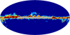 |
Fig. 3 HEALPix masks with growing fsky (Nside = 32): 85% (dark blue), 90% (light blue), 92% (green), 95% (orange), and 97.3% (brown). The 97.3% mask additionally excludes the inner Galactic plane within 3 degrees of latitude and pixels within 4 degrees of the Crab pulsar (gray). |
4.2 Data simulations, debiasing, and error-bars estimation
To assess uncertainties associated with Planck satellite noise, including systematics, and the CMB signal, we computed a set of simulated maps based on various models of dust polarization from PYSM 3 (Thorne et al. 2017; Zonca et al. 2021; Group 2025). The d1 model is built from the Planck 353 GHz Legacy maps, extrapolated at lower frequencies with an MBB spectrum, using the spatially varying temperature and spectral index obtained from the Planck intensity data with the Commander code (Planck Collaboration 2015 X 2016). The d10 model is a refined version of d1, in which the templates for amplitude and spectral parameters have been extracted from the GNILC analysis of the Planck data (Planck Collaboration Int. XLVIII 2016; Planck Collaboration 2018 XII 2020), with smaller scales included using the so-called logarithm of the polarization fraction tensor formalism (for more details, see Group (2025)). Finally, the d12 model consists of up to six superposed layers of modified black bodies, each with spectral parameters drawn from Gaussian distributions (Martínez-Solaeche et al. 2018). The dust model maps were combined with the SRoll2 simulations of data noise and systematics (Delouis et al. 2019) and with CMB maps computed from the CMB power spectrum for the ΛCDM fiducial Planck model (Planck Collaboration 2018 VI 2020) as described in Sect. 3.2 of Ritacco et al. (2023). Overall, at each of the four Planck frequencies, we obtained Nsims = 200 sets of simulated Q and U full and half-mission maps, with independent realizations of data uncertainties and CMB anisotropies. The simulations were treated identically to the Planck data.
Our model is designed to study the frequency dependence of the variances, c, of dust polarized emission. The Planck data must be corrected for the bias introduced by noise, systematics, and the CMB in the raw data squared quantities, craw. For simulation number k, the bias introduced by noise, systematics, and the CMB on any squared quantity, c, is estimated as
![Mathematical equation: $\[c_{\text {bias }}(k) \equiv c_{\text {sims }}(k)-c_{\mathrm{dm}},\]$](/articles/aa/full_html/2026/01/aa56491-25/aa56491-25-eq125.png) (40)
(40)
where csims(k) and cdm represent the covariances of simulation k and of the chosen PYSM 3 dust model, respectively. Taking the raw biased data value craw, we obtain, for each simulation k, a debiased estimate, ![Mathematical equation: $\[\hat{c}(k)\]$](/articles/aa/full_html/2026/01/aa56491-25/aa56491-25-eq126.png) , for the covariance, c(k), in the Planck SRoll2 data:
, for the covariance, c(k), in the Planck SRoll2 data:
![Mathematical equation: $\[\hat{c}(k) \equiv c_{\mathrm{raw}}-c_{\mathrm{bias}}(k)=c_{\mathrm{raw}}-c_{\mathrm{sims}}(k)+c_{\mathrm{dm}}.\]$](/articles/aa/full_html/2026/01/aa56491-25/aa56491-25-eq127.png) (41)
(41)
The debiased value, c, and its uncertainty, σc, are taken as the mean and standard deviation of ![Mathematical equation: $\[\hat{c}(k)\]$](/articles/aa/full_html/2026/01/aa56491-25/aa56491-25-eq128.png) over its 200 values, respectively.
over its 200 values, respectively.
From now on, we present only the results obtained using d1, our reference model. The results obtained using d10 and d12 are presented in the Appendix F; they do not differ significantly from those presented below, ensuring the robustness of our conclusions against the dust model used in our debiasing procedure.
4.3 Mean complex polarized SED
We extended earlier studies (Planck Collaboration Int. XXX 2016; Planck Collaboration 2018 XI 2020; Ritacco et al. 2023) to the complex plane using the cross-correlation of Planck maps, and determined the mean, debiased, complex SED ![Mathematical equation: $\[\overline{\mathbf{r}}_{i}\]$](/articles/aa/full_html/2026/01/aa56491-25/aa56491-25-eq129.png) of dust polarization, normalized to our reference channel,
of dust polarization, normalized to our reference channel,
![Mathematical equation: $\[\overline{\mathbf{r}}_i \equiv \frac{\tilde{\rho}_i \tilde{\rho}_0\left\langle\mathbf{P}_i \mathbf{P}_0^{\star}\right\rangle_{\mathrm{raw}}-\frac{1}{N_{\text {sims }}} \sum_{k=1}^{N_{\text {sims }}}\left\langle\mathbf{P}_i \mathbf{P}_0^{\star}\right\rangle_{\mathrm{sim} ~k}+\left\langle\mathbf{P}_i \mathbf{P}_0^{\star}\right\rangle_{\mathrm{dm}}}{\tilde{\rho}_0^2\left\langle\mathbf{P}_0 \mathbf{P}_0^{\star}\right\rangle_{\mathrm{raw}}-\frac{1}{N_{\text {sims }}} \sum_{k=1}^{N_{\text {sims }}}\left\langle\mathbf{P}_0 \mathbf{P}_0^{\star}\right\rangle_{\mathrm{sim} ~k}+\left\langle\mathbf{P}_0 \mathbf{P}_0^{\star}\right\rangle_{\mathrm{dm}}},\]$](/articles/aa/full_html/2026/01/aa56491-25/aa56491-25-eq130.png) (42)
(42)
where ![Mathematical equation: $\[\tilde{\rho}_{i}\]$](/articles/aa/full_html/2026/01/aa56491-25/aa56491-25-eq131.png) is the correction to the polarization efficiency7 at frequency νi (Ritacco et al. 2023, Table 1). Similarly, we computed
is the correction to the polarization efficiency7 at frequency νi (Ritacco et al. 2023, Table 1). Similarly, we computed ![Mathematical equation: $\[\mathbf{r}_{i}^{\mathrm{dm}} \equiv\left\langle\mathbf{P}_{i} \mathbf{P}_{0}^{\star}\right\rangle_{\mathrm{dm}} /\left\langle\mathbf{P}_{0} \mathbf{P}_{0}^{\star}\right\rangle_{\mathrm{dm}}\]$](/articles/aa/full_html/2026/01/aa56491-25/aa56491-25-eq132.png) for the dust model,
for the dust model, ![Mathematical equation: $\[\mathbf{r}_{i}^{\text {sim}}(k) \equiv\left\langle\mathbf{P}_{i} \mathbf{P}_{0}^{\star}\right\rangle_{k} /\left\langle\mathbf{P}_{0} \mathbf{P}_{0}^{\star}\right\rangle_{k}\]$](/articles/aa/full_html/2026/01/aa56491-25/aa56491-25-eq133.png) for simulation k, and
for simulation k, and ![Mathematical equation: $\[\overline{\mathbf{r}}_{i}^{\text {sims}} \equiv {\sum}_{k=1}^{N_{\text {sims}}}\left\langle\mathbf{P}_{i} \mathbf{P}_{0}^{\star}\right\rangle_{k} / {\sum}_{k=1}^{N_{\text {sims}}}\left\langle\mathbf{P}_{0} \mathbf{P}_{0}^{\star}\right\rangle_{k}\]$](/articles/aa/full_html/2026/01/aa56491-25/aa56491-25-eq134.png) for the mean of all simulations.
for the mean of all simulations.
The uncertainty on the real and imaginary components of the mean simulated SED ![Mathematical equation: $\[\overline{\mathbf{r}}_{i}^{\text {sims}}\]$](/articles/aa/full_html/2026/01/aa56491-25/aa56491-25-eq135.png) is taken as the standard deviation of the corresponding real and imaginary components of the 200 simulation values
is taken as the standard deviation of the corresponding real and imaginary components of the 200 simulation values ![Mathematical equation: $\[\mathbf{r}_{i}^{\text {sim}}(k)\]$](/articles/aa/full_html/2026/01/aa56491-25/aa56491-25-eq136.png) . The uncertainty in the observed SED
. The uncertainty in the observed SED ![Mathematical equation: $\[\overline{\mathbf{r}}_{i}\]$](/articles/aa/full_html/2026/01/aa56491-25/aa56491-25-eq137.png) must also include the uncertainty in the recalibration factor,
must also include the uncertainty in the recalibration factor, ![Mathematical equation: $\[\tilde{\rho}_{i}\]$](/articles/aa/full_html/2026/01/aa56491-25/aa56491-25-eq138.png) , of the Planck polarization data:
, of the Planck polarization data: ![Mathematical equation: $\[\sigma\left(\tilde{\rho}_{i}\right) / \tilde{\rho}_{i}=0.5 \%\]$](/articles/aa/full_html/2026/01/aa56491-25/aa56491-25-eq139.png) . We repeated the procedure described in Sect. 4.2 200 times, each time drawing a distinct recalibration factor for each channel, i, from a random Gaussian distribution of expectation
. We repeated the procedure described in Sect. 4.2 200 times, each time drawing a distinct recalibration factor for each channel, i, from a random Gaussian distribution of expectation ![Mathematical equation: $\[\tilde{\rho}_{i}\]$](/articles/aa/full_html/2026/01/aa56491-25/aa56491-25-eq140.png) and standard deviation
and standard deviation ![Mathematical equation: $\[\sigma\left(\tilde{\rho}_{i}\right)=0.005 \tilde{\rho}_{i}\]$](/articles/aa/full_html/2026/01/aa56491-25/aa56491-25-eq141.png) . We debiased this realization with simulation k alone to compute the kth debiased estimate
. We debiased this realization with simulation k alone to compute the kth debiased estimate ![Mathematical equation: $\[\hat{\mathbf{r}}_{i}(k)\]$](/articles/aa/full_html/2026/01/aa56491-25/aa56491-25-eq142.png) of
of ![Mathematical equation: $\[\overline{\mathbf{r}}_{i}\]$](/articles/aa/full_html/2026/01/aa56491-25/aa56491-25-eq143.png) . The uncertainty in the real and imaginary parts of
. The uncertainty in the real and imaginary parts of ![Mathematical equation: $\[\overline{\mathbf{r}}_{i}\]$](/articles/aa/full_html/2026/01/aa56491-25/aa56491-25-eq144.png) is then taken as the standard deviation of the real and imaginary components of this set of 200 values
is then taken as the standard deviation of the real and imaginary components of this set of 200 values ![Mathematical equation: $\[\hat{\mathbf{r}}_{i}(k)\]$](/articles/aa/full_html/2026/01/aa56491-25/aa56491-25-eq145.png) , respectively. To test the assumption made in Sect. 2.5 to obtain Eq. (20), we computed the module of
, respectively. To test the assumption made in Sect. 2.5 to obtain Eq. (20), we computed the module of ![Mathematical equation: $\[\overline{\mathbf{r}}_{i} \frac{\overline{\varepsilon}_{0}}{\overline{\varepsilon}_{i}}-1\]$](/articles/aa/full_html/2026/01/aa56491-25/aa56491-25-eq146.png) for a pivot SED,
for a pivot SED, ![Mathematical equation: $\[\overline{\varepsilon}_{i}\]$](/articles/aa/full_html/2026/01/aa56491-25/aa56491-25-eq147.png) , fitted to
, fitted to ![Mathematical equation: $\[\overline{\mathbf{r}}_{i}\]$](/articles/aa/full_html/2026/01/aa56491-25/aa56491-25-eq148.png) , and found it smaller than 0.03 at all frequencies.
, and found it smaller than 0.03 at all frequencies.
Figure 4 shows the spectral dependence of the mean complex polarized SED in the log complex plane, for the raw SRoll2 data, the mean of simulations, the d1 dust model used for debiasing and the resulting debiased SED ![Mathematical equation: $\[\overline{\mathbf{r}}_{i}\]$](/articles/aa/full_html/2026/01/aa56491-25/aa56491-25-eq149.png) . We observe a variation of the polarization angle with frequency in the data, which may appear significant. However, our estimate for the uncertainty on
. We observe a variation of the polarization angle with frequency in the data, which may appear significant. However, our estimate for the uncertainty on ![Mathematical equation: $\[\overline{\mathbf{r}}_{i}\]$](/articles/aa/full_html/2026/01/aa56491-25/aa56491-25-eq150.png) does not include the uncertainty in the orientation of the Planck polarization bolometers. The most stringent estimates of these uncertainties come from the analysis of EB cross-spectra carried out to constrain cosmic birefringence (Planck Collaboration Int. XLIX 2016; Minami & Komatsu 2020; Diego-Palazuelos et al. 2022, 2023). Diego-Palazuelos et al. (2022) list their results in Table 1, per bolometer for several Galactic masks. The scatter among Galactic masks and the statistical uncertainties both lie in the range 0.2–0.3°. This agrees with the systematic uncertainty of 0.28° quoted by Planck Collaboration Int. XLIX (2016). The magnitude of this uncertainty reduces the significance of the imaginary component of our mean SED.
does not include the uncertainty in the orientation of the Planck polarization bolometers. The most stringent estimates of these uncertainties come from the analysis of EB cross-spectra carried out to constrain cosmic birefringence (Planck Collaboration Int. XLIX 2016; Minami & Komatsu 2020; Diego-Palazuelos et al. 2022, 2023). Diego-Palazuelos et al. (2022) list their results in Table 1, per bolometer for several Galactic masks. The scatter among Galactic masks and the statistical uncertainties both lie in the range 0.2–0.3°. This agrees with the systematic uncertainty of 0.28° quoted by Planck Collaboration Int. XLIX (2016). The magnitude of this uncertainty reduces the significance of the imaginary component of our mean SED.
While the mean complex SED, ![Mathematical equation: $\[\overline{\mathbf{r}}_{i}\]$](/articles/aa/full_html/2026/01/aa56491-25/aa56491-25-eq156.png) , depends on calibration errors in amplitude (correction factors
, depends on calibration errors in amplitude (correction factors ![Mathematical equation: $\[\tilde{\rho}_{i}\]$](/articles/aa/full_html/2026/01/aa56491-25/aa56491-25-eq157.png) ) and in phase (absolute orientation of bolometers in the focal plane), the definition of map residuals (Eq. (18)), involving the ratio of Pi to
) and in phase (absolute orientation of bolometers in the focal plane), the definition of map residuals (Eq. (18)), involving the ratio of Pi to ![Mathematical equation: $\[\overline{\mathbf{r}}_{i}\]$](/articles/aa/full_html/2026/01/aa56491-25/aa56491-25-eq158.png) , renders the map residuals, and therefore their covariances, independent of any calibration error, whether in amplitude or in phase. This facilitates the comparison of different frequency maps or datasets with distinct systematics.
, renders the map residuals, and therefore their covariances, independent of any calibration error, whether in amplitude or in phase. This facilitates the comparison of different frequency maps or datasets with distinct systematics.
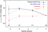 |
Fig. 4 Mean complex polarized SED |
![Mathematical equation: $\[\overline{\mathbf{r}}_{i}\]$](/articles/aa/full_html/2026/01/aa56491-25/aa56491-25-eq151.png)
4.4 Comparison of model predictions with Planck polarization data
In this section, we compare our model predictions and hypotheses with the Planck SRoll2 data. Using simulations, we have verified that the 0.5% in the recalibration factors ![Mathematical equation: $\[\tilde{\rho}_{i}\]$](/articles/aa/full_html/2026/01/aa56491-25/aa56491-25-eq159.png) does not have a noticeable effect on our results.
does not have a noticeable effect on our results.
First, we tested model prediction P1 by computing the Pearson correlation coefficient ![Mathematical equation: $\[\rho_{i j}=c_{i j} / \sqrt{c_{i i} c_{j j}}\]$](/articles/aa/full_html/2026/01/aa56491-25/aa56491-25-eq160.png) , between the residual maps i and j. Our results for the R, RP, and Rψ residual maps are presented in Table 1 for all frequency pairs, using our 97.3% mask. The error bars on ρij are calculated from the standard deviation of the simulated values ρij(k), following the approach described in Sect. 4.2. We find that the correlation coefficient between the RP residual maps is consistent with a perfect correlation. The correlation between the angle residual maps, Rψ, is strong for the (217,143) pair, but weak for the (143,100) and (100,217) pairs, although with large uncertainties. Therefore, prediction P1 is validated for RP but not for Rψ. The correlation coefficient of Re cP is high but only marginally compatible with 100% for the (217,100) and (143,100) pairs. In the context of Eq. (33), this loss of correlation between the residual maps Ri is a consequence of the loss of correlation between the residual maps
, between the residual maps i and j. Our results for the R, RP, and Rψ residual maps are presented in Table 1 for all frequency pairs, using our 97.3% mask. The error bars on ρij are calculated from the standard deviation of the simulated values ρij(k), following the approach described in Sect. 4.2. We find that the correlation coefficient between the RP residual maps is consistent with a perfect correlation. The correlation between the angle residual maps, Rψ, is strong for the (217,143) pair, but weak for the (143,100) and (100,217) pairs, although with large uncertainties. Therefore, prediction P1 is validated for RP but not for Rψ. The correlation coefficient of Re cP is high but only marginally compatible with 100% for the (217,100) and (143,100) pairs. In the context of Eq. (33), this loss of correlation between the residual maps Ri is a consequence of the loss of correlation between the residual maps ![Mathematical equation: $\[R_{i}^{\psi}\]$](/articles/aa/full_html/2026/01/aa56491-25/aa56491-25-eq161.png) .
.
Second, we examined the validity of predictions P2 and P3, which relate cε and cψ to ![Mathematical equation: $\[\left\langle P_{0}^{2}\right\rangle\]$](/articles/aa/full_html/2026/01/aa56491-25/aa56491-25-eq164.png) and
and ![Mathematical equation: $\[\left\langle I_{0}^{2}\right\rangle\]$](/articles/aa/full_html/2026/01/aa56491-25/aa56491-25-eq165.png) , respectively. Fig. 5 shows how the variances, computed at 217 GHz for a high S/N ratio, depend on the polarization fraction, p0, at 353 GHz. This correlation plot is obtained by binning pixels of the 97.3% mask in bins of p0 and computing, for each p0 bin, the variances c at 217 GHzand the mean squared values,
, respectively. Fig. 5 shows how the variances, computed at 217 GHz for a high S/N ratio, depend on the polarization fraction, p0, at 353 GHz. This correlation plot is obtained by binning pixels of the 97.3% mask in bins of p0 and computing, for each p0 bin, the variances c at 217 GHzand the mean squared values, ![Mathematical equation: $\[\left\langle P_{0}^{2}\right\rangle\]$](/articles/aa/full_html/2026/01/aa56491-25/aa56491-25-eq166.png) and
and ![Mathematical equation: $\[\left\langle I_{0}^{2}\right\rangle\]$](/articles/aa/full_html/2026/01/aa56491-25/aa56491-25-eq167.png) (a method only applicable at the map level). A model,
(a method only applicable at the map level). A model, ![Mathematical equation: $\[c^{\varepsilon} \propto\left\langle P_{0}^{2}\right\rangle\]$](/articles/aa/full_html/2026/01/aa56491-25/aa56491-25-eq168.png) , shown as a dashed orange line, confirms our prediction P2. Another model,
, shown as a dashed orange line, confirms our prediction P2. Another model, ![Mathematical equation: $\[c^{\psi} \propto\left\langle I_{0}^{2}\right\rangle\]$](/articles/aa/full_html/2026/01/aa56491-25/aa56491-25-eq169.png) (dashed red line), also confirms the surprising prediction P3 of our model: cψ is reasonably proportional to
(dashed red line), also confirms the surprising prediction P3 of our model: cψ is reasonably proportional to ![Mathematical equation: $\[\left\langle I_{0}^{2}\right\rangle\]$](/articles/aa/full_html/2026/01/aa56491-25/aa56491-25-eq170.png) , rather than
, rather than ![Mathematical equation: $\[\left\langle P_{0}^{2}\right\rangle\]$](/articles/aa/full_html/2026/01/aa56491-25/aa56491-25-eq171.png) . Consequently, while cε follows
. Consequently, while cε follows ![Mathematical equation: $\[\left\langle P_{0}^{2}\right\rangle\]$](/articles/aa/full_html/2026/01/aa56491-25/aa56491-25-eq172.png) as the polarization fraction tends toward zero, cP and Re cP saturate at positive values (prediction P4) due to depolarization effects (the variance of which is quantified here by cψ) that persist even at low p0.
as the polarization fraction tends toward zero, cP and Re cP saturate at positive values (prediction P4) due to depolarization effects (the variance of which is quantified here by cψ) that persist even at low p0.
Predictions P5 and P6 are compared to Planck SRoll2 data in Fig. 6, which shows how the ratio ![Mathematical equation: $\[c_{i j}^{\psi} / c_{i j}^{P}\]$](/articles/aa/full_html/2026/01/aa56491-25/aa56491-25-eq173.png) varies with fsky, for all pairs (i, j) of residual maps. The error bars for this ratio are computed from simulations, following the approach described in Sect. 4.2. Prediction P5 (
varies with fsky, for all pairs (i, j) of residual maps. The error bars for this ratio are computed from simulations, following the approach described in Sect. 4.2. Prediction P5 (![Mathematical equation: $\[c^{\psi} / c^{P} \leq 1 / \overline{\eta}\]$](/articles/aa/full_html/2026/01/aa56491-25/aa56491-25-eq174.png) , unhashed region) is verified for all frequency pairs except for the variances at 100 and 143 GHz at lower fsky. This indicates that either the hypotheses of our model or the debiasing method break down at lower fsky. For the 95 and 97.3% masks, the cψ/cP ratio is, within error bars, almost independent of the frequency pair considered (prediction P6), with the notable exception of the variance at 100 GHz.
, unhashed region) is verified for all frequency pairs except for the variances at 100 and 143 GHz at lower fsky. This indicates that either the hypotheses of our model or the debiasing method break down at lower fsky. For the 95 and 97.3% masks, the cψ/cP ratio is, within error bars, almost independent of the frequency pair considered (prediction P6), with the notable exception of the variance at 100 GHz.
Overall, Table 1 and Fig. 6 highlight a limitation of our approach for the 100 GHz channel. In Sect. 6, we discuss to what extent this distinctive behavior can be attributed to dust physics beyond our hypotheses, to residual contamination by a component other than dust and CMB (e.g., synchrotron or CO emission), or to limitations of our debiasing method.
Finally, in Table 2, we test prediction P7, which states that ![Mathematical equation: $\[\operatorname{Im} \mathbf{c}_{i j}^{\mathbf{P}}\]$](/articles/aa/full_html/2026/01/aa56491-25/aa56491-25-eq177.png) should be, within the uncertainties, close to zero for all frequency pairs. This prediction is not verified, even for the frequency pair (217,143) for which the residual maps show the strongest correlation (see Table 1). This result is puzzling, as our model does not predict any correlation between Rψ and RP, except for chance correlation. This issue is examined in more detail in the following section.
should be, within the uncertainties, close to zero for all frequency pairs. This prediction is not verified, even for the frequency pair (217,143) for which the residual maps show the strongest correlation (see Table 1). This result is puzzling, as our model does not predict any correlation between Rψ and RP, except for chance correlation. This issue is examined in more detail in the following section.
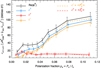 |
Fig. 5 Test of predictions P2, P3, and P4: dependence on the observed polarization fraction p0 = P0/I0 at 353 GHz of the variances Re cP, cP, cψ, and cε computed at 217 GHz. Our models for cε (P2) and cψ (P3) are overplotted as dotted orange and red lines, respectively, using the mean value of the slope derived from these equations, multiplied by |
![Mathematical equation: $\[\left\langle P_{0}^{2}\right\rangle\]$](/articles/aa/full_html/2026/01/aa56491-25/aa56491-25-eq162.png)
![Mathematical equation: $\[\left\langle I_{0}^{2}\right\rangle\]$](/articles/aa/full_html/2026/01/aa56491-25/aa56491-25-eq163.png)
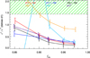 |
Fig. 6 Test of predictions P5 and P6 as a function of fsky. The hashed region represents forbidden values according to P5. |
5 Inferring the variance of the spectral properties of aligned grains
Polarization observations trace the spectral properties of a specific population of dust grains that are aligned with the magnetic field lines. They can be compared with the overall spectral properties inferred from dust far-infrared (FIR) and submm total emission, which trace all grains, both aligned and unaligned. Assuming a common temperature8 for aligned and unaligned grains, Planck Collaboration 2018 XI (2020) found close values for the mean spectral index in polarization and intensity: βP − βI = 0.05 ± 0.03 in the high-latitude diffuse ISM. In this section, we extend this work by quantifying the variance of the fluctuations in the spectral properties of aligned grains for the 97.3% mask, where the signal is dominated by the Galactic plane. We trace these variations back to their origin in the fluctuations of β or T, and correlate them with the spectral fluctuations observed in total intensity.
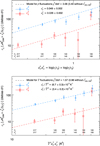 |
Fig. 7 Comparison of SRoll2 data with the predictions of our model for cP (blue) and cψ (red), for pure β fluctuations (top), and pure T fluctuations (bottom). |
5.1 Disentangling fluctuations of dust temperature and spectral index
As demonstrated in Sect. 3.1, the spectral gradients ![Mathematical equation: $\[a_{i, n}^{s}\]$](/articles/aa/full_html/2026/01/aa56491-25/aa56491-25-eq178.png) for n = 2 and n = 3 are strongly correlated with
for n = 2 and n = 3 are strongly correlated with ![Mathematical equation: $\[a_{i, 1}^{s}\]$](/articles/aa/full_html/2026/01/aa56491-25/aa56491-25-eq179.png) . By correlating the covariance matrices
. By correlating the covariance matrices ![Mathematical equation: $\[c_{i j}^{P}\]$](/articles/aa/full_html/2026/01/aa56491-25/aa56491-25-eq180.png) and
and ![Mathematical equation: $\[c_{i j}^{\psi}\]$](/articles/aa/full_html/2026/01/aa56491-25/aa56491-25-eq181.png) with
with ![Mathematical equation: $\[a_{i, 1}^{\beta} a_{j, 1}^{\beta}\]$](/articles/aa/full_html/2026/01/aa56491-25/aa56491-25-eq182.png) and
and ![Mathematical equation: $\[\overline{T}^{4} a_{i, 1}^{T} a_{j, 1}^{T}\]$](/articles/aa/full_html/2026/01/aa56491-25/aa56491-25-eq183.png) separately9, we aimed to identify whether these fluctuations originated mainly from variations in β or T, while simultaneously estimating their amplitude. This analysis is illustrated in Fig. 7 for pure β fluctuations (labeled (top)) and pure T fluctuations (labeled (bottom)). The spectral trends observed for cP and cψ are not compatible with a scenario in which they originate from fluctuations in β, as this scenario predicts a steeper slope. A better agreement is obtained if only the dust temperature T fluctuates. In the Galactic plane, starlight heating may indeed dominate the fluctuations of dust emission properties. For the variance in angles (cψ), fluctuations in T may also be favored, although the significant contamination observed in the 100 GHz residual angle map prevents a firm conclusion. To quantify these trends, we performed a χ2 minimization using the MPFITCOVAR IDL routine (Markwardt 2009). Our data combine the two data sets,
separately9, we aimed to identify whether these fluctuations originated mainly from variations in β or T, while simultaneously estimating their amplitude. This analysis is illustrated in Fig. 7 for pure β fluctuations (labeled (top)) and pure T fluctuations (labeled (bottom)). The spectral trends observed for cP and cψ are not compatible with a scenario in which they originate from fluctuations in β, as this scenario predicts a steeper slope. A better agreement is obtained if only the dust temperature T fluctuates. In the Galactic plane, starlight heating may indeed dominate the fluctuations of dust emission properties. For the variance in angles (cψ), fluctuations in T may also be favored, although the significant contamination observed in the 100 GHz residual angle map prevents a firm conclusion. To quantify these trends, we performed a χ2 minimization using the MPFITCOVAR IDL routine (Markwardt 2009). Our data combine the two data sets, ![Mathematical equation: $\[c_{i j}^{P}\]$](/articles/aa/full_html/2026/01/aa56491-25/aa56491-25-eq184.png) and
and ![Mathematical equation: $\[c_{i j}^{\psi}\]$](/articles/aa/full_html/2026/01/aa56491-25/aa56491-25-eq185.png) , into an array of 12 values. The corresponding 12 × 12 noise covariance matrix was computed from the covariances between the 200 simulated
, into an array of 12 values. The corresponding 12 × 12 noise covariance matrix was computed from the covariances between the 200 simulated ![Mathematical equation: $\[c_{i j}^{P}(k)\]$](/articles/aa/full_html/2026/01/aa56491-25/aa56491-25-eq186.png) and
and ![Mathematical equation: $\[c_{i j}^{\psi}(k)\]$](/articles/aa/full_html/2026/01/aa56491-25/aa56491-25-eq187.png) covariance matrices (see Sect. 4.2). Using predictions P2, P3, and P4, we define a linear model for fluctuations in the spectral parameter s ∈ {T, β}, where
covariance matrices (see Sect. 4.2). Using predictions P2, P3, and P4, we define a linear model for fluctuations in the spectral parameter s ∈ {T, β}, where ![Mathematical equation: $\[c_{i j}^{\psi}=a_{i, 1}^{s} a_{j, 1}^{s}\left(\sigma_{s}^{\psi}\right)^{2}\left\langle P_{0}^{2}\right\rangle\]$](/articles/aa/full_html/2026/01/aa56491-25/aa56491-25-eq188.png) and
and ![Mathematical equation: $\[c_{i j}^{P}= a_{i, 1}^{s} a_{j, 1}^{s}\left(\sigma_{s}^{\varepsilon}\right)^{2}\left\langle P_{0}^{2}\right\rangle+\overline{\eta} c_{i j}^{\psi}\]$](/articles/aa/full_html/2026/01/aa56491-25/aa56491-25-eq189.png) , with
, with ![Mathematical equation: $\[\sigma_{s}^{\psi} \equiv \sqrt{\operatorname{Cov}\left(\operatorname{Im\boldsymbol{\mathcal{W}}}_{\mathbf{1}}^{s}, \operatorname{Im \boldsymbol{\mathcal{W}}}_{\mathbf{1}}^{s}\right)}\]$](/articles/aa/full_html/2026/01/aa56491-25/aa56491-25-eq190.png) and
and ![Mathematical equation: $\[\sigma_{s}^{\varepsilon} \equiv \sqrt{\operatorname{Cov}\left(\omega_{1}^{s}, \omega_{1}^{s}\right)}\]$](/articles/aa/full_html/2026/01/aa56491-25/aa56491-25-eq191.png) . When fitting with pure fluctuations in T, we obtain a χ2 of 15.7 (or 1.57 per degree of freedom). For pure β fluctuations, χ2 increases to 31. Removing
. When fitting with pure fluctuations in T, we obtain a χ2 of 15.7 (or 1.57 per degree of freedom). For pure β fluctuations, χ2 increases to 31. Removing ![Mathematical equation: $\[c_{100 \times 100}^{\psi}\]$](/articles/aa/full_html/2026/01/aa56491-25/aa56491-25-eq192.png) from the dataset clearly improves the fit for fluctuations in T (χ2/dof = 0.96), but not for fluctuations in β. Changing the value of
from the dataset clearly improves the fit for fluctuations in T (χ2/dof = 0.96), but not for fluctuations in β. Changing the value of ![Mathematical equation: $\[\overline{\eta}\]$](/articles/aa/full_html/2026/01/aa56491-25/aa56491-25-eq193.png) does not affect the χ2 of the fit’ it modifies only the value of
does not affect the χ2 of the fit’ it modifies only the value of ![Mathematical equation: $\[\sigma_{s}^{\varepsilon}\]$](/articles/aa/full_html/2026/01/aa56491-25/aa56491-25-eq194.png) , while keeping
, while keeping ![Mathematical equation: $\[\left(\sigma_{s}^{\varepsilon}\right)^{2}+\overline{\eta}\left(\sigma_{s}^{\psi}\right)^{2}\]$](/articles/aa/full_html/2026/01/aa56491-25/aa56491-25-eq195.png) constant. Our best fit provides a reasonable value for the typical dispersion in dust temperature in the Galactic plane, corresponding to
constant. Our best fit provides a reasonable value for the typical dispersion in dust temperature in the Galactic plane, corresponding to ![Mathematical equation: $\[\sigma_{T}^{\varepsilon}=(2.7 \pm 0.1) ~\mathrm{K}\]$](/articles/aa/full_html/2026/01/aa56491-25/aa56491-25-eq196.png) for a reference temperature
for a reference temperature ![Mathematical equation: $\[\overline{T}=20 \mathrm{~K}\]$](/articles/aa/full_html/2026/01/aa56491-25/aa56491-25-eq197.png) .
.
Finally, Fig. 8 shows the frequency dependence of the mixed covariances ![Mathematical equation: $\[c_{i j}^{\psi P}\]$](/articles/aa/full_html/2026/01/aa56491-25/aa56491-25-eq199.png) (Eq. (28)). This graph confirms that the 143 GHz channel behaves differently from the 217 and 100 GHz channels, possibly indicating contamination by CO emission in these two channels (see Sect. 6). A first-order model (dashed line) based on fluctuations of the dust temperature,
(Eq. (28)). This graph confirms that the 143 GHz channel behaves differently from the 217 and 100 GHz channels, possibly indicating contamination by CO emission in these two channels (see Sect. 6). A first-order model (dashed line) based on fluctuations of the dust temperature, ![Mathematical equation: $\[c_{i j}^{\psi P}=a_{i, 1}^{T} a_{j, 1}^{T} \Sigma_{T}^{\psi P}\left\langle P_{0}^{2}\right\rangle\]$](/articles/aa/full_html/2026/01/aa56491-25/aa56491-25-eq200.png) , with
, with ![Mathematical equation: $\[\Sigma_{T}^{\psi P} \equiv \operatorname{Cov}\left(\operatorname{Im\boldsymbol{\mathcal{W}}}_{\mathbf{1}}^{\boldsymbol{T}}, \operatorname{Re \boldsymbol{\mathcal{W}}}_{\mathbf{1}}^{\boldsymbol{T}}\right)\]$](/articles/aa/full_html/2026/01/aa56491-25/aa56491-25-eq201.png) , cannot reproduce the observations. A model based on fluctuations in β also fails. The frequency dependence of the mixed covariances
, cannot reproduce the observations. A model based on fluctuations in β also fails. The frequency dependence of the mixed covariances ![Mathematical equation: $\[c_{i j}^{\psi P}\]$](/articles/aa/full_html/2026/01/aa56491-25/aa56491-25-eq202.png) , together with the values of
, together with the values of ![Mathematical equation: $\[\operatorname{Im} \mathbf{c}_{i j}^{\mathbf{P}}\]$](/articles/aa/full_html/2026/01/aa56491-25/aa56491-25-eq203.png) (Table 2), warrants further detailed analysis. We defer this to future work.
(Table 2), warrants further detailed analysis. We defer this to future work.
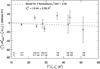 |
Fig. 8 Covariances |
![Mathematical equation: $\[c_{i j}^{\psi P}\]$](/articles/aa/full_html/2026/01/aa56491-25/aa56491-25-eq198.png)
5.2 Correlating fluctuations in intensity and polarization
We next correlated the fluctuations observed in the dust polarized emissivity with the fluctuations observed in total intensity. We used the d1 dust model, based on Commander total intensity maps, as a proxy for the dust emissivity fluctuations in total intensity. This model does not include any significant decorrelation in angles (see Sect. 4.1), which implies that Rψ(d1) ≃ 0 and cP(d1) ≃ cε(d1). Correlating RP(SR) from the SRoll2 data with RP(d1) from the d1 dust model therefore quantifies the variance of dust emissivity common to both residual maps, independently of the variance in angles present in the Planck SRoll2 maps RP(SR). Figure 9 compares the dependence with the frequency νi of the variance ![Mathematical equation: $\[c_{i i}^{\varepsilon}\]$](/articles/aa/full_html/2026/01/aa56491-25/aa56491-25-eq204.png) (SR) of the SRoll2 data, of the variance
(SR) of the SRoll2 data, of the variance ![Mathematical equation: $\[c_{i i}^{\varepsilon}\]$](/articles/aa/full_html/2026/01/aa56491-25/aa56491-25-eq205.png) (d1) =
(d1) = ![Mathematical equation: $\[c_{i i}^{P}\]$](/articles/aa/full_html/2026/01/aa56491-25/aa56491-25-eq206.png) (d1) of the d1 dust model, and their cross-covariance,
(d1) of the d1 dust model, and their cross-covariance,
![Mathematical equation: $\[c_{i i}^P(\mathrm{~d} 1 \times \mathrm{SR}) \equiv\left\langle R_i^P(\mathrm{~d} 1) \times R_i^P(\mathrm{SR})\right\rangle.\]$](/articles/aa/full_html/2026/01/aa56491-25/aa56491-25-eq207.png) (43)
(43)
Fig. 9 shows that the variance of emissivity of aligned grains (as traced by cε(SR)) and that of all grains (aligned or unaligned, traced by cP(d1)), are of compatible amplitude, except at 217 GHz. The SRoll2 polarization data follow a T trend, while the d1 intensity data lie between the pure T and pure β trends. The data-model correlation coefficients,
![Mathematical equation: $\[\rho_i^{\varepsilon}(\mathrm{d} 1 \times \mathrm{SR})=c_{i i}^P(\mathrm{~d} 1 \times \mathrm{SR}) / \sqrt{c_{i i}^{\varepsilon}(\mathrm{SR}) \times c_{i i}^P(\mathrm{~d} 1)},\]$](/articles/aa/full_html/2026/01/aa56491-25/aa56491-25-eq208.png) (44)
(44)
are relatively high (above 85%) at all frequencies. However, the value at 100 GHz must be interpreted with caution, as the value derived for ![Mathematical equation: $\[c_{100 \times 100}^{\varepsilon}\]$](/articles/aa/full_html/2026/01/aa56491-25/aa56491-25-eq209.png) through Eq. (39) is underestimated due to contamination by
through Eq. (39) is underestimated due to contamination by ![Mathematical equation: $\[c_{100 \times 100}^{\psi}\]$](/articles/aa/full_html/2026/01/aa56491-25/aa56491-25-eq210.png) , as observed in Fig. 7. Overall, this indicates that the fluctuations observed in the total SED of a given light cone correspond closely to the fluctuations present in the polarized SED of the same light cone.
, as observed in Fig. 7. Overall, this indicates that the fluctuations observed in the total SED of a given light cone correspond closely to the fluctuations present in the polarized SED of the same light cone.
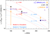 |
Fig. 9 Comparison of the spectral dependence of covariances cε from SRoll2 data, cP for the dust model d1, and cP for the cross-product of SRoll2 and d1. The Pearson correlation coefficient ρ(d1, SR) is indicated (purple). Predictions for models with T or β fluctuations are overplotted. |
5.3 Results obtained with the Planck PR4 data release
In Appendix E, we present figures and tables obtained using the same methodology but applied to the last official release of Planck data, PR4. Our goal was not to show a preference for one data release over another, but to demonstrate that our methodology can quantify differences between datasets and track their origin. Despite the clear differences in the mean complex SED, our assessment of the seven predictions remains the same. The main difference between these two data releases appears in the spectral dependence of covariances. The PR4 and SRoll2 covariances, cP and cψ, are compatible within uncertainties, except for ![Mathematical equation: $\[c_{217 \times 217}^{P}\]$](/articles/aa/full_html/2026/01/aa56491-25/aa56491-25-eq211.png) and
and ![Mathematical equation: $\[c_{100 \times 100}^{\psi}\]$](/articles/aa/full_html/2026/01/aa56491-25/aa56491-25-eq212.png) , possibly indicating a distinct handling of contamination by CO emission. The PR4 and SRoll2 cψP mixed covariances are compatible for all channel pairs. Contamination of the 100 GHz channel appears to be significant in cP in the PR4 data, unlike in SRoll2. Finally, while the SRoll2 data shows a preference for pure fluctuations in T, PR4 data, with χ2/dof ≃ 14, are not compatible with a dust model assuming either pure fluctuations in T or in β, even when excluding
, possibly indicating a distinct handling of contamination by CO emission. The PR4 and SRoll2 cψP mixed covariances are compatible for all channel pairs. Contamination of the 100 GHz channel appears to be significant in cP in the PR4 data, unlike in SRoll2. Finally, while the SRoll2 data shows a preference for pure fluctuations in T, PR4 data, with χ2/dof ≃ 14, are not compatible with a dust model assuming either pure fluctuations in T or in β, even when excluding ![Mathematical equation: $\[c_{100 \times 100}^{\psi}\]$](/articles/aa/full_html/2026/01/aa56491-25/aa56491-25-eq213.png) and
and ![Mathematical equation: $\[c_{100 \times 100}^{P}\]$](/articles/aa/full_html/2026/01/aa56491-25/aa56491-25-eq214.png) . Our methodology reveals clear differences between the SRoll2 and PR4 data, particularly in the mean properties and variances of the 217 and 100 GHz channels contaminated by CO leakage.
. Our methodology reveals clear differences between the SRoll2 and PR4 data, particularly in the mean properties and variances of the 217 and 100 GHz channels contaminated by CO leakage.
5.4 Dependence on the dust model used for debiasing
The influence of our debiasing method (Sect. 4.2), applied with the d1 dust model, is tested in Appendix F using the d10 and d12 PySM 3 dust models. This effect is weak and does not alter our conclusions. However, the fact that no dust model includes a frequency-rotation of polarization angles at the pixel level (with the exception of d12, which does not appear to behave realistically, as indicated by the negative Pearson coefficients in Fig. F.4) is clearly problematic. One of the goals of this article is to propose new diagnostics for developing such models. Coupling these diagnostics with model-building tools based on moment expansion, as proposed by Vacher et al. (2025), could provide a powerful combination to provide new, realistic, and complex foreground models anchored in data.
6 Discussion
Our model, based on simple hypotheses, makes strong predictions and testable predictions. Its success enables the measure of the variance in the spectral properties of aligned grains. Its limitations provide new insights into the origins of the imperfect correlation observed in polarization angle residual maps.
6.1 Insights into the properties of aligned grains
Correlating fluctuations in the polarized SED with those observed in total intensity, we find a strong, though not perfect, correlation (ρ > 85%; Fig. 9). This behavior is expected. What we call dust grains are actually a set of grain populations with distinct composition, optical properties, and alignment properties (Shiu et al. 2024; Siebenmorgen 2023). Typically, small grains and possibly unaligned large carbonaceous grains do not emit in polarization (Kim & Martin 1995; Chiar et al. 2006). Maps of total intensity collect the thermal emission from all grains, whether aligned or not with the magnetic field. Because the impact of magnetic fields on fluctuations in the polarized SED is statistically mitigated within our methodology, the strong correlation between intensity and polarization residual maps leads us to conclude that the emission from aligned grains is highly dominant in Planck channels, compared with that from unaligned grains.
As a second result on dust properties, we find that the frequency-dependence of the variance of these fluctuations is consistent only with variations in dust temperature T, showing no indication of a variation in the dust spectral index β. This result may be specific to the low Galactic latitudes that dominate our signal, where the light cone samples the systematic increase in the radiation-field intensity toward the molecular, star-forming ring of the Galaxy. However, we do not draw firm conclusions from this preliminary result. Firstly, it is at odds with those drawn from analyses of FIR and submm total-intensity SEDs (Ysard et al. 2013; Planck Collaboration 2013 XI 2014; Planck Collaboration Int. XVII 2014) and from a recent evolution of dust models (Ysard et al. 2024), and secondly, because it is not confirmed using the PR4 version of the Planck data (see Sect. 5.3). This apparent contradiction requires further investigation.
6.2 Investigating the origin of the imperfect correlation of polarization angle residuals
Our model predicts a perfect correlation between the polarization SEDs and angles residuals (but not of the polarized SEDs themselves). Analyzing the Planck SRoll2 data with this model, we find that fluctuations of the submm polarized SED are indeed strongly correlated (ρP > 90%; Table 1) across frequencies for the polarized intensity, Pν, but only weakly correlated for the polarization angles, ψν. The level of correlation between residual maps is lower with PR4, but remains similar (see Appendix E). This raises the question of which physical processes or components could be responsible for the weaker-than-expected correlation observed between the polarization angle residual maps.
Dust itself could be the origin of part of this loss of correlation. First, we restricted our MBB modeling to the simple situation (hypothesis HM3), where only T or β vary in the sky, not both. Observations show that, in total intensity, both T and β vary within any given region of the sky. The possible correlation between T and β has also been the subject of a long series of studies (Dupac et al. 2003; Anderson et al. 2010; Planck Collaboration 2011 XXIV 2011; Planck Collaboration 2013 XI 2014). All of these studies are based on intensity rather than polarization maps, which motivated our simple hypothesis HM3. Nevertheless, the impact of simultaneous variations, possibly correlated or anti-correlated, of T and β on our analysis remains to be explored. Second, the predicted 100% correlation between frequencies for fluctuations in T derives from the law of blackbody thermal emission and is therefore as strict as a physical law. In contrast, fluctuations in β represent a simplification of what may truly occur. This simplification assumes that variations in the FIR and submm dust emissivity, Qabs(ν), are perfectly correlated across frequencies. Laboratory data do not support this assumption (Demyk et al. 2022). The prediction of a 100% correlation for fluctuations in β is therefore not derived from solid physics, but from our simplifying hypothesis HA1, the MBB model. Finally, through the same hypothesis HA1, our study neglects refinements of dust models, such as variations in dust cooling efficiency (Ysard et al. 2024), the magnetic dipole emission of dust grains (Draine & Hensley 2013), which may produce polarized emission around 100 GHz with a polarization direction perpendicular to the magnetic field, or the polarized emission by a population of very large (up to 1 μm) grains that may have distinct dust properties (Siebenmorgen 2023). In summary, the predicted 100% correlation of map residuals between frequencies strongly relies on our hypothesis HA1, and is therefore questionable.
Within the framework of our hypothesis HM6, we also ignore any component other than dust, the CMB, and Planck noise and systematics. The removal of synchrotron polarized emission from the 143 and 100 GHz maps (see Sect. 4.1) may have left some residuals. There is also a significant component that is not included in the simulations, as it is difficult to model: the possible leakage of CO line emission into polarized Stokes maps Q and U, in the 100 and 217 GHz channels. In the Galactic plane, CO emission arises from various regions of the Galaxy, with distinct radial velocities and therefore distinct CO line emission frequencies. Because each Planck HFI bolometer that measures linear polarization has its own spectral transfer efficiency, a leakage from intensity to polarization is observed. This artificial polarization, absent from the 143 GHz channel, contributes to the observed decorrelation of polarization angles, as well as to the distortion in the spectral dependence of their covariances shown in Fig. 7. It can also affect the spectral dependence of the mean SED (Fig. 4). Finally, CO molecules may also have an unexpected effect on the measurement of dust polarization by Planck. Anisotropic resonant scattering of background dust polarized emission by foreground aligned CO molecules (Houde et al. 2013; Hezareh et al. 2013) can induce a rotation of the dust polarization signal, potentially affecting the correlation of angles in the 217 and 100 GHz channels, while leaving the 143 GHz channel uncontaminated.
7 Summary and conclusions
We have presented an analytical framework for interpreting variations in the submillimeter polarized SED in terms of fluctuations in spectral properties, T and β, of aligned grains across the sky and within the light cones of observation. Following Vacher et al. (2023b), our approach is based on complex quantities, allowing for a consistent treatment of the fluctuations in the spectral parameters of the polarized SED and of the spectral rotation of angles, isolated in distinct residual maps. When either T or β fluctuates, our model predicts an almost perfect correlation across frequencies between all dust polarization residual maps. The decorrelation observed in the Stokes parameters Qν and Uν translates into a perfect frequency-correlation of Pν in the complex plane.
Following Ritacco et al. (2023), we validated our model using Planck SRoll2 data (Delouis et al. 2019), with a fsky = 97.3% mask excluding the inner Galactic plane. To characterize fluctuations in dust polarization properties, covariances of residual maps were computed at the map level, and debiased from contamination by the CMB, noise, and systematics using 200 end-to-end simulations. We find that polarized-intensity residual maps are strongly correlated across frequencies, while polarization angle residual maps are weakly correlated for the (217,143) and (217,100) GHz pairs and uncorrelated for the (143,100) GHz pair. This departure from the predicted perfect correlation between residual maps is discussed in the context of dust physics and data analysis. Polarized SED fluctuations are dominated by variations in the dust temperature (σT ~ 2.7 K, assuming a mean temperature ![Mathematical equation: $\[\overline{T}=20 \mathrm{~K}\]$](/articles/aa/full_html/2026/01/aa56491-25/aa56491-25-eq215.png) for aligned grains), excluding any significant contribution from fluctuations in the dust polarization spectral index, β. In our analysis, dominated by the Galactic plane, fluctuations in the dust emissivity observed in the polarization SED at all frequencies are strongly correlated with those traced by Commander PR2 maps characterizing the dust SED in total intensity (Planck Collaboration 2015 X 2016), implying that emission from aligned grains greatly exceeds emission by non-aligned grains in the submillimeter. These results, based on SRoll2 maps, are compatible with those obtained using the latest official Planck release, PR4, following the same methodology, with the notable exception that the spectral dependence of the covariances computed with PR4 data is not compatible with a dust model assuming pure fluctuations in either T or β.
for aligned grains), excluding any significant contribution from fluctuations in the dust polarization spectral index, β. In our analysis, dominated by the Galactic plane, fluctuations in the dust emissivity observed in the polarization SED at all frequencies are strongly correlated with those traced by Commander PR2 maps characterizing the dust SED in total intensity (Planck Collaboration 2015 X 2016), implying that emission from aligned grains greatly exceeds emission by non-aligned grains in the submillimeter. These results, based on SRoll2 maps, are compatible with those obtained using the latest official Planck release, PR4, following the same methodology, with the notable exception that the spectral dependence of the covariances computed with PR4 data is not compatible with a dust model assuming pure fluctuations in either T or β.
Observations of dust emission in polarization provide access to a new dimension of dust evolution, inaccessible to unpolarized observations: the statistics of dust properties variations within the light cone (2D within the beam and 3D along the line of sight). This information appears in what we call the “spectral rotation of polarization angles.” Our model captures a significant fraction of the decorrelation in angles found in Planck data, as well as the variance observed in dust unpolarized-emission SEDs. The spatial variation of the SED induced by rotation of the polarization angle along the line of sight is a critical aspect that could strongly affect the detection of CMB B-modes and any other attempts to detect cosmic birefringence. Our methodology, which is independent of calibration errors and can be used with any mask, enables correlation analyses with tracers of the ISM to trace the origin of decorrelation. This work is useful and timely for the development of component-separation methods for current and future generations of CMB experiments. It will aid the development of new, more realistic sky simulations that include SED decorrelation with amplitudes consistent with Planck data.
Acknowledgements
V.G. thanks M. Houde for interesting discussions. L.V. acknowledges partial support by the Italian Space Agency LiteBIRD Project (ASI Grants No. 2020-9-HH.0 and 2016-24-H.1-2018), as well as the Radio-ForegroundsPlus Project HORIZON-CL4-2023-SPACE-01, GA 101135036 and through the Project SPACE-IT-UP by the Italian Space Agency and Ministry of University and Research, Contract Number 2024-5-E.0. A.R. acknowledges financial support from the Italian Ministry of University and Research – Project Proposal CIR01_00010. A.B. acknowledges financial support from the INAF initiative “IAF Astronomy Fellowships in Italy” (grant name MEGASKAT).
References
- Anderson, L. D., Zavagno, A., Rodón, J. A., et al. 2010, A&A, 518, L99 [NASA ADS] [CrossRef] [EDP Sciences] [Google Scholar]
- Azzoni, S., Abitbol, M. H., Alonso, D., et al. 2021, J. Cosmology Astropart. Phys., 2021, 047 [Google Scholar]
- Azzoni, S., Alonso, D., Abitbol, M. H., Errard, J., & Krachmalnicoff, N. 2023, J. Cosmology Astropart. Phys., 2023, 035 [Google Scholar]
- Carones, A., & Remazeilles, M. 2024, J. Cosmology Astropart. Phys., 2024, 018 [Google Scholar]
- Chiar, J. E., Adamson, A. J., Whittet, D. C. B., et al. 2006, ApJ, 651, 268 [CrossRef] [Google Scholar]
- Chluba, J., Hill, J. C., & Abitbol, M. H. 2017, MNRAS, 472, 1195 [NASA ADS] [CrossRef] [Google Scholar]
- Clark, S. E., & Hensley, B. S. 2019, ApJ, 887, 136 [NASA ADS] [CrossRef] [Google Scholar]
- Delouis, J. M., Pagano, L., Mottet, S., Puget, J. L., & Vibert, L. 2019, A&A, 629, A38 [NASA ADS] [CrossRef] [EDP Sciences] [Google Scholar]
- Demyk, K., Meny, C., Lu, X. H., et al. 2022, A&A, 666, C3 [NASA ADS] [CrossRef] [EDP Sciences] [Google Scholar]
- Désert, F.-X. 2022, A&A, 659, A70 [NASA ADS] [CrossRef] [EDP Sciences] [Google Scholar]
- Diego-Palazuelos, P., Eskilt, J. R., Minami, Y., et al. 2022, Phys. Rev. Lett., 128, 091302 [NASA ADS] [CrossRef] [Google Scholar]
- Diego-Palazuelos, P., Martínez-González, E., Vielva, P., et al. 2023, J. Cosmology Astropart. Phys., 2023, 044 [Google Scholar]
- Draine, B. T. 2003, ARA&A, 41, 241 [NASA ADS] [CrossRef] [Google Scholar]
- Draine, B. T., & Hensley, B. 2013, ApJ, 765, 159 [Google Scholar]
- Dupac, X., Bernard, J. P., Boudet, N., et al. 2003, A&A, 404, L11 [NASA ADS] [CrossRef] [EDP Sciences] [Google Scholar]
- Fanciullo, L., Guillet, V., Aniano, G., et al. 2015, A&A, 580, A136 [NASA ADS] [CrossRef] [EDP Sciences] [Google Scholar]
- Ghosh, T., Boulanger, F., Martin, P. G., et al. 2017, A&A, 601, A71 [NASA ADS] [CrossRef] [EDP Sciences] [Google Scholar]
- Górski, K. M., Hivon, E., Banday, A. J., et al. 2005, ApJ, 622, 759 [Google Scholar]
- Group, T. P.-E. G. S. 2025, submitted to ApJ [arXiv:2502.20452] [Google Scholar]
- Hensley, B. S., & Draine, B. T. 2023, ApJ, 948, 55 [Google Scholar]
- Hezareh, T., Wiesemeyer, H., Houde, M., Gusdorf, A., & Siringo, G. 2013, A&A, 558, A45 [NASA ADS] [CrossRef] [EDP Sciences] [Google Scholar]
- Houde, M., Hezareh, T., Jones, S., & Rajabi, F. 2013, ApJ, 764, 24 [NASA ADS] [CrossRef] [Google Scholar]
- Jenkins, E. B. 2009, ApJ, 700, 1299 [Google Scholar]
- Jost, B., Errard, J., & Stompor, R. 2023, Phys. Rev. D, 108, 082005 [Google Scholar]
- Kim, S.-H., & Martin, P. G. 1995, ApJ, 444, 293 [Google Scholar]
- LiteBIRD Collaboration 2022, PTEP, 11443, 114432F [Google Scholar]
- Markwardt, C. B. 2009, ASP Conf. Ser., 411, 251 [Google Scholar]
- Martínez-Solaeche, G., Karakci, A., & Delabrouille, J. 2018, MNRAS, 476, 1310 [Google Scholar]
- McBride, L., Bull, P., & Hensley, B. S. 2023, MNRAS, 519, 4370 [NASA ADS] [CrossRef] [Google Scholar]
- Minami, Y., & Komatsu, E. 2020, Phys. Rev. Lett., 125, 221301 [NASA ADS] [CrossRef] [Google Scholar]
- Pelgrims, V., Clark, S. E., Hensley, B. S., et al. 2021, A&A, 647, A16 [NASA ADS] [CrossRef] [EDP Sciences] [Google Scholar]
- Planck Collaboration 2011 XXIV. 2011, A&A, 536, A25 [NASA ADS] [CrossRef] [EDP Sciences] [Google Scholar]
- Planck Collaboration 2013 XI. 2014, A&A, 571, A11 [NASA ADS] [CrossRef] [EDP Sciences] [Google Scholar]
- Planck Collaboration 2015 X. 2016, A&A, 594, A10 [NASA ADS] [CrossRef] [EDP Sciences] [Google Scholar]
- Planck Collaboration 2018 VI. 2020, A&A, 641, A6 [NASA ADS] [CrossRef] [EDP Sciences] [Google Scholar]
- Planck Collaboration 2018 XI. 2020, A&A, 641, A11 [NASA ADS] [CrossRef] [EDP Sciences] [Google Scholar]
- Planck Collaboration 2018 XII. 2020, A&A, 641, A12 [NASA ADS] [CrossRef] [EDP Sciences] [Google Scholar]
- Planck Collaboration Int. XVII. 2014, A&A, 566, A55 [NASA ADS] [CrossRef] [EDP Sciences] [Google Scholar]
- Planck Collaboration Int. XIX. 2015, A&A, 576, A104 [NASA ADS] [CrossRef] [EDP Sciences] [Google Scholar]
- Planck Collaboration Int. XXX. 2016, A&A, 586, A133 [NASA ADS] [CrossRef] [EDP Sciences] [Google Scholar]
- Planck Collaboration Int. XLIV. 2016, A&A, 596, A105 [NASA ADS] [CrossRef] [EDP Sciences] [Google Scholar]
- Planck Collaboration Int. XLVIII. 2016, A&A, 596, A109 [NASA ADS] [CrossRef] [EDP Sciences] [Google Scholar]
- Planck Collaboration Int. XLIX. 2016, A&A, 596, A110 [NASA ADS] [CrossRef] [EDP Sciences] [Google Scholar]
- Planck Collaboration Int. L. 2017, A&A, 599, A51 [NASA ADS] [CrossRef] [EDP Sciences] [Google Scholar]
- Planck Collaboration Int. LVII. 2020, A&A, 643, A42 [NASA ADS] [CrossRef] [EDP Sciences] [Google Scholar]
- Remazeilles, M., Dickinson, C., Eriksen, H. K. K., & Wehus, I. K. 2016, MNRAS, 458, 2032 [Google Scholar]
- Remazeilles, M., Rotti, A., & Chluba, J. 2021, MNRAS, 503, 2478 [NASA ADS] [CrossRef] [Google Scholar]
- Ritacco, A., Boulanger, F., Guillet, V., et al. 2023, A&A, 670, A163 [NASA ADS] [CrossRef] [EDP Sciences] [Google Scholar]
- Schlafly, E. F., Meisner, A. M., Stutz, A. M., et al. 2016, ApJ, 821, 78 [NASA ADS] [CrossRef] [Google Scholar]
- Shiu, C., Benton, S. J., Filippini, J. P., et al. 2024, ApJ, 970, 43 [Google Scholar]
- Siebenmorgen, R. 2023, A&A, 670, A115 [NASA ADS] [CrossRef] [EDP Sciences] [Google Scholar]
- Sponseller, D., & Kogut, A. 2022, ApJ, 936, 8 [NASA ADS] [CrossRef] [Google Scholar]
- Sullivan, R. M., Abghari, A., Diego-Palazuelos, P., Hergt, L. T., & Scott, D. 2025, J. Cosmology Astropart. Phys., 2025, 025 [Google Scholar]
- Tassis, K., & Pavlidou, V. 2015, MNRAS, 451, L90 [NASA ADS] [CrossRef] [Google Scholar]
- Thorne, B., Dunkley, J., Alonso, D., & Næss, S. 2017, MNRAS, 469, 2821 [Google Scholar]
- Vacher, L., Aumont, J., Montier, L., et al. 2022, A&A, 660, A111 [NASA ADS] [CrossRef] [EDP Sciences] [Google Scholar]
- Vacher, L., Aumont, J., Boulanger, F., et al. 2023a, A&A, 672, A146 [NASA ADS] [CrossRef] [EDP Sciences] [Google Scholar]
- Vacher, L., Chluba, J., Aumont, J., Rotti, A., & Montier, L. 2023b, A&A, 669, A5 [NASA ADS] [CrossRef] [EDP Sciences] [Google Scholar]
- Vacher, L., Carones, A., Aumont, J., et al. 2025, A&A, 697, A212 [NASA ADS] [CrossRef] [EDP Sciences] [Google Scholar]
- Vansyngel, F., Boulanger, F., Ghosh, T., et al. 2017, A&A, 603, A62 [NASA ADS] [CrossRef] [EDP Sciences] [Google Scholar]
- Wolz, K., Azzoni, S., Hervías-Caimapo, C., et al. 2024, A&A, 686, A16 [NASA ADS] [CrossRef] [EDP Sciences] [Google Scholar]
- Ysard, N., Abergel, A., Ristorcelli, I., et al. 2013, A&A, 559, A133 [NASA ADS] [CrossRef] [EDP Sciences] [Google Scholar]
- Ysard, N., Jones, A. P., Guillet, V., et al. 2024, A&A, 684, A34 [NASA ADS] [CrossRef] [EDP Sciences] [Google Scholar]
- Zaldarriaga, M. & Seljak, U. 1997, Phys. Rev. D, 55, 1830 [Google Scholar]
- Zonca, A., Thorne, B., Krachmalnicoff, N., & Borrill, J. 2021, J. Open Source Softw., 6, 3783 [NASA ADS] [CrossRef] [Google Scholar]
To emit polarized thermal emission, dust grains must be aligned with the local magnetic field. Not all grains are aligned: it has been proven that grains smaller than ~0.1 μm are not aligned (e.g., Kim & Martin 1995), while the existence of a population of large, unaligned, possibly carbonaceous grains remains debated (Chiar et al. 2006; Siebenmorgen 2023; Hensley & Draine 2023; Ysard et al. 2024).
Here, the spin-moments are defined alternatively, as in Vacher et al. (2023b), with the correspondence Pν0 ≡ 𝒲0 and ![Mathematical equation: $\[\boldsymbol{\mathcal{W}}_{1}^{s} \equiv \boldsymbol{\mathcal{W}}_{1}^{s} / \boldsymbol{\mathcal{W}}_{0}\]$](/articles/aa/full_html/2026/01/aa56491-25/aa56491-25-eq315.png) . This redefinition of the first-order moment is more operational but valid only in the perturbative regime
. This redefinition of the first-order moment is more operational but valid only in the perturbative regime ![Mathematical equation: $\[\boldsymbol{\mathcal{W}}_{0} \gg \boldsymbol{\mathcal{W}}_{1}^{s}\]$](/articles/aa/full_html/2026/01/aa56491-25/aa56491-25-eq316.png) , a condition that which we assume here (for a discussion, see Vacher et al. 2023b,a).
, a condition that which we assume here (for a discussion, see Vacher et al. 2023b,a).
The relatively large uncertainty in ![Mathematical equation: $\[\overline{\eta}\]$](/articles/aa/full_html/2026/01/aa56491-25/aa56491-25-eq317.png) accounts for the simplifications used in these estimations.
accounts for the simplifications used in these estimations.
There is no correction for the 353 GHz channel (![Mathematical equation: $\[\tilde{\rho}_{0}=1\]$](/articles/aa/full_html/2026/01/aa56491-25/aa56491-25-eq318.png) ). The relative uncertainty on
). The relative uncertainty on ![Mathematical equation: $\[\tilde{\rho}_{i}\]$](/articles/aa/full_html/2026/01/aa56491-25/aa56491-25-eq319.png) is
is ![Mathematical equation: $\[\sigma_{\tilde{\rho}} / \tilde{\rho}=0.5 \%\]$](/articles/aa/full_html/2026/01/aa56491-25/aa56491-25-eq320.png) for all channels (Ritacco et al. 2023).
for all channels (Ritacco et al. 2023).
Lacking high-frequency channels in polarization, the temperature of aligned grains could not be measured from Planck polarization data.
While ![Mathematical equation: $\[a_{\nu, 1}^{\beta}\]$](/articles/aa/full_html/2026/01/aa56491-25/aa56491-25-eq321.png) is independent of
is independent of ![Mathematical equation: $\[\overline{\beta}, a_{\nu, 1}^{T}\]$](/articles/aa/full_html/2026/01/aa56491-25/aa56491-25-eq322.png) depends on
depends on ![Mathematical equation: $\[\overline{T}\]$](/articles/aa/full_html/2026/01/aa56491-25/aa56491-25-eq323.png) . The expression
. The expression ![Mathematical equation: $\[\overline{T}^{2} a_{\nu, 1}^{T}\]$](/articles/aa/full_html/2026/01/aa56491-25/aa56491-25-eq324.png) depends only weakly on
depends only weakly on ![Mathematical equation: $\[\overline{T}\]$](/articles/aa/full_html/2026/01/aa56491-25/aa56491-25-eq325.png) , with less than 10% variation when
, with less than 10% variation when ![Mathematical equation: $\[\overline{T}\]$](/articles/aa/full_html/2026/01/aa56491-25/aa56491-25-eq326.png) spans a range between 15 and 25 K.
spans a range between 15 and 25 K.
The value of P0 for ~1% of pixels having ![Mathematical equation: $\[\operatorname{Re}\left(\mathbf{P}_{0}^{\mathrm{HM} 1} \times\left(\mathbf{P}_{0}^{\mathrm{HM} 2}\right)^{\star}\right)<0\]$](/articles/aa/full_html/2026/01/aa56491-25/aa56491-25-eq327.png) has been forced to zero, with no noticeable impact on our analysis.
has been forced to zero, with no noticeable impact on our analysis.
Appendix A Dictionary of defined quantities
Table A.1 presents all our defined quantities, with references to equations, sections, figures and tables.
Dictionary of all defined quantities, with complex quantities in bold.
Appendix B Relation between the intensity-weighted and polarization-weighted moments of spectral parameters
The polarization-weighted ![Mathematical equation: $\[\boldsymbol{\mathcal{W}}_{n}^{s}\]$](/articles/aa/full_html/2026/01/aa56491-25/aa56491-25-eq252.png) and intensity-weighted
and intensity-weighted ![Mathematical equation: $\[\omega_{n}^{s}\]$](/articles/aa/full_html/2026/01/aa56491-25/aa56491-25-eq253.png) spinmoments quantify the same statistics within the light cone, the moments of the fluctuations of spectral parameter s of aligned grains, but with a distinct weight. In this section, we show that
spinmoments quantify the same statistics within the light cone, the moments of the fluctuations of spectral parameter s of aligned grains, but with a distinct weight. In this section, we show that ![Mathematical equation: $\[\Delta_{n}^{s} \equiv \boldsymbol{\mathcal{W}}_{n}^{s}-\omega_{n}^{s}\]$](/articles/aa/full_html/2026/01/aa56491-25/aa56491-25-eq254.png) is of zero mean.
is of zero mean.
We first introduce the local (unobserved) complex polarization fraction
![Mathematical equation: $\[\hat{\mathbf{p}} \equiv \frac{\mathrm{d} \mathbf{P}}{\mathrm{~d} I},\]$](/articles/aa/full_html/2026/01/aa56491-25/aa56491-25-eq255.png) (B.1)
(B.1)
covered by ∧ to be distinguished from the observed complex polarization fraction
![Mathematical equation: $\[\mathbf{p} \equiv \frac{\mathbf{P}}{I}.\]$](/articles/aa/full_html/2026/01/aa56491-25/aa56491-25-eq256.png) (B.2)
(B.2)
We have
![Mathematical equation: $\[\mathbf{P}=\int_{\mathcal{L}} \mathrm{d} \mathbf{P}=\int_{\mathcal{L}} \hat{\mathbf{p}} ~\mathrm{d} I.\]$](/articles/aa/full_html/2026/01/aa56491-25/aa56491-25-eq257.png) (B.3)
(B.3)
Using Eq. (B.1) and (B.2), Eq. (8) defining ![Mathematical equation: $\[\boldsymbol{\mathcal{W}}_{n}^{s}\]$](/articles/aa/full_html/2026/01/aa56491-25/aa56491-25-eq258.png) becomes, expressed this time in terms of an integral over the total intensity I:
becomes, expressed this time in terms of an integral over the total intensity I:
![Mathematical equation: $\[\boldsymbol{\mathcal{W}}_n^s=\frac{1}{I} \int_{\mathcal{L}}(s-\overline{s})^n \frac{\hat{\mathbf{p}}}{\mathbf{p}} \mathrm{~d} I,\]$](/articles/aa/full_html/2026/01/aa56491-25/aa56491-25-eq259.png) (B.4)
(B.4)
so that
![Mathematical equation: $\[\Delta_n^s \equiv \boldsymbol{\mathcal{W}}_n^s-\omega_n^s=\frac{1}{I} \int_{\mathcal{L}}(s-\overline{s})^n \delta \hat{\mathbf{p}} \mathrm{~d} I,\]$](/articles/aa/full_html/2026/01/aa56491-25/aa56491-25-eq260.png) (B.5)
(B.5)
where
![Mathematical equation: $\[\delta \hat{\mathbf{p}} \equiv\left(\frac{\hat{\mathbf{p}}}{\mathbf{p}}-1\right)\]$](/articles/aa/full_html/2026/01/aa56491-25/aa56491-25-eq261.png) (B.6)
(B.6)
is the complex quantity characterizing the departure of the local complex polarization fraction ![Mathematical equation: $\[\hat{\mathbf{p}}\]$](/articles/aa/full_html/2026/01/aa56491-25/aa56491-25-eq262.png) from the observed complex polarization fraction p.
from the observed complex polarization fraction p.
When integrated over the light cone, the quantity ![Mathematical equation: $\[\delta \hat{\mathbf{p}}\]$](/articles/aa/full_html/2026/01/aa56491-25/aa56491-25-eq263.png) has by definition a mean value of zero:
has by definition a mean value of zero:
![Mathematical equation: $\[\int_{\mathcal{L}} \delta \hat{\mathbf{p}} ~\mathrm{d} I=\left(\frac{1}{\mathbf{p}} \int_{\mathcal{L}} \hat{\mathbf{p}} ~\mathrm{d} I\right)-I=\frac{1}{\mathbf{p}}\left(\int_{\mathcal{L}} \mathrm{d} \mathbf{P}\right)-I=\mathbf{0}.\]$](/articles/aa/full_html/2026/01/aa56491-25/aa56491-25-eq264.png) (B.7)
(B.7)
As a consequence, from Eq. (B.5) we conclude that ![Mathematical equation: $\[\Delta_{n}^{s}\]$](/articles/aa/full_html/2026/01/aa56491-25/aa56491-25-eq265.png) is also of zero mean under our hypothesis HA2 of no correlation between the structure of the magnetic field and the variations of dust temperature and spectral index.
is also of zero mean under our hypothesis HA2 of no correlation between the structure of the magnetic field and the variations of dust temperature and spectral index.
Appendix C Toy model for line of sight integration
In this appendix, we make again use of the phenomenological model of the submillimeter polarized thermal dust emission, developed in Planck Collaboration Int. XLIV (2016), Ghosh et al. (2017), and Vansyngel et al. (2017). This simple model proved successful to explain different statistical properties of polarization quantities (Planck Collaboration Int. XLIV 2016; Planck Collaboration 2018 XII 2020).
We decompose the Galactic sky into N layers of equal intensity I0/N. Each layer k (k ∈ [1 . . . N]) has a uniform magnetic field ![Mathematical equation: $\[\overrightarrow{\boldsymbol{B}}_{k}=\overrightarrow{\boldsymbol{B}}_{0}+\overrightarrow{\Delta \boldsymbol{B}}_{k}\]$](/articles/aa/full_html/2026/01/aa56491-25/aa56491-25-eq266.png) , sum of an ordered component
, sum of an ordered component ![Mathematical equation: $\[\overrightarrow{\boldsymbol{B}}_{0}\]$](/articles/aa/full_html/2026/01/aa56491-25/aa56491-25-eq267.png) (a uniform Galactic magnetic field) and of a random component
(a uniform Galactic magnetic field) and of a random component ![Mathematical equation: $\[\overrightarrow{\Delta B}_{k}\]$](/articles/aa/full_html/2026/01/aa56491-25/aa56491-25-eq268.png) , following our hypothesis HM5. The turbulent component
, following our hypothesis HM5. The turbulent component ![Mathematical equation: $\[\overrightarrow{\Delta B}_{k}\]$](/articles/aa/full_html/2026/01/aa56491-25/aa56491-25-eq269.png) in each layer is a realization of an isotropic Gaussian random field in three dimensions, of variance
in each layer is a realization of an isotropic Gaussian random field in three dimensions, of variance ![Mathematical equation: $\[\sigma_{B}^{2}\]$](/articles/aa/full_html/2026/01/aa56491-25/aa56491-25-eq270.png) . The random and ordered components are taken close to equipartition (fM ≡ σB/B0 ≃ 1) in order to match observational properties (Planck Collaboration 2018 XII 2020).
. The random and ordered components are taken close to equipartition (fM ≡ σB/B0 ≃ 1) in order to match observational properties (Planck Collaboration 2018 XII 2020).
Our model provides two maps of angles for each layer k: one γ(k) for the inclination angle of the magnetic field with respect to the plane of the sky, and one ψ(k) for the projection of the magnetic field onto the plane of the sky, rotated by 90°. We use this model to quantify the variance of the real and imaginary parts of ![Mathematical equation: $\[\delta \hat{\mathbf{p}}^{(k)}\]$](/articles/aa/full_html/2026/01/aa56491-25/aa56491-25-eq271.png) (Eq. (B.6)), where p is the observed, light coneintegrated, complex polarization fraction, while
(Eq. (B.6)), where p is the observed, light coneintegrated, complex polarization fraction, while ![Mathematical equation: $\[\hat{\mathbf{p}}^{(k)}\]$](/articles/aa/full_html/2026/01/aa56491-25/aa56491-25-eq272.png) is the local uniform polarization fraction in layer k. Assuming that the grain alignment efficiency is uniform in the sky (our hypothesis HA4) with a maximal polarization fraction pmax, we have the following expressions:
is the local uniform polarization fraction in layer k. Assuming that the grain alignment efficiency is uniform in the sky (our hypothesis HA4) with a maximal polarization fraction pmax, we have the following expressions:
![Mathematical equation: $\[\hat{\mathbf{p}}^{(k)}=p_{\text {max }} \cos ^2 \gamma^{(k)} \mathrm{e}^{\dot{\mathbb{i}} 2 \psi^{(k)}},\]$](/articles/aa/full_html/2026/01/aa56491-25/aa56491-25-eq273.png) (C.1)
(C.1)
![Mathematical equation: $\[\mathbf{p}=\frac{1}{N} \sum_{k=1}^N \hat{\mathbf{p}}^{(k)}.\]$](/articles/aa/full_html/2026/01/aa56491-25/aa56491-25-eq274.png) (C.2)
(C.2)
Fig. C.1 shows the dependency, with the normalized polarization fraction p/pmax, of the mean value of the variance of ![Mathematical equation: $\[\operatorname{Re} \delta \hat{\mathbf{p}}^{(k)}\]$](/articles/aa/full_html/2026/01/aa56491-25/aa56491-25-eq275.png) , of the variance of
, of the variance of ![Mathematical equation: $\[\operatorname{Im} \delta \hat{\mathbf{p}}^{(k)}\]$](/articles/aa/full_html/2026/01/aa56491-25/aa56491-25-eq276.png) and of their ratio, for three values of the number N of layers and five values of σB/B0 comprised between 0.7 and 1.1 (all combinations compatible within uncertainties with Planck data). In the top and middle panel, the variance
and of their ratio, for three values of the number N of layers and five values of σB/B0 comprised between 0.7 and 1.1 (all combinations compatible within uncertainties with Planck data). In the top and middle panel, the variance ![Mathematical equation: $\[\sigma_{\operatorname{Re \delta \hat{\mathbf{p}}}}^{2}\]$](/articles/aa/full_html/2026/01/aa56491-25/aa56491-25-eq277.png) and
and ![Mathematical equation: $\[\sigma_{\operatorname{Im \delta \hat{\mathbf{p}}}}^{2}\]$](/articles/aa/full_html/2026/01/aa56491-25/aa56491-25-eq278.png) are found to be inversely correlated with p2 at low values of p, but with a departure from this trend at high p. To characterize the distinct dependence of
are found to be inversely correlated with p2 at low values of p, but with a departure from this trend at high p. To characterize the distinct dependence of ![Mathematical equation: $\[\sigma_{\operatorname{Re \delta \hat{\mathbf{p}}}}^{2}\]$](/articles/aa/full_html/2026/01/aa56491-25/aa56491-25-eq279.png) and
and ![Mathematical equation: $\[\sigma_{\operatorname{Im \delta \hat{\mathbf{p}}}}^{2}\]$](/articles/aa/full_html/2026/01/aa56491-25/aa56491-25-eq280.png) with p, we study how their ratio η varies with p
with p, we study how their ratio η varies with p
![Mathematical equation: $\[\eta(p) \equiv \frac{\sigma_{\operatorname{Re \delta \hat{\mathbf{p}}}}^2(p)}{\sigma_{\operatorname{Im \delta \hat{\mathbf{p}}}}^2(p)}.\]$](/articles/aa/full_html/2026/01/aa56491-25/aa56491-25-eq281.png) (C.3)
(C.3)
The ratio η(p) shows a clear decreasing trend with p (Fig. C.1, bottom panel). The higher the polarization fraction, the more the spectral variations in angles dominate over the spectral variation in the polarized intensity SED. This effect is strong at low polarization fractions (as η(0) ≃ 1), and weak or undetected at high polarization fractions (η(pmax) = 0). Modeling the dependence of η with p is beyond the scope of this paper. Our first goal is to take into account the dependence of ![Mathematical equation: $\[\sigma_{\operatorname{Im \delta \hat{\mathbf{p}}}}^{2}\]$](/articles/aa/full_html/2026/01/aa56491-25/aa56491-25-eq282.png) and
and ![Mathematical equation: $\[\sigma_{\operatorname{Re \delta \hat{\mathbf{p}}}}^{2}\]$](/articles/aa/full_html/2026/01/aa56491-25/aa56491-25-eq283.png) in 1/p2, not their second order dependence through their ratio η(p). Therefore, as a reference value, we ignore our mask and simply take the mean value of η(p) over the full-sky:
in 1/p2, not their second order dependence through their ratio η(p). Therefore, as a reference value, we ignore our mask and simply take the mean value of η(p) over the full-sky: ![Mathematical equation: $\[\overline{\eta} \simeq 0.7 \pm 0.2\]$](/articles/aa/full_html/2026/01/aa56491-25/aa56491-25-eq284.png) . The significant uncertainty is here to acknowledge for the crude approximation we have by ignoring the p-dependence of η. Our mask is dominated by regions with low p (p353 < 0.4pmax) at 4° of resolution, where η(p) does not vary too much, making our approximation reasonable. In this frame, we have the approximate relation
. The significant uncertainty is here to acknowledge for the crude approximation we have by ignoring the p-dependence of η. Our mask is dominated by regions with low p (p353 < 0.4pmax) at 4° of resolution, where η(p) does not vary too much, making our approximation reasonable. In this frame, we have the approximate relation
![Mathematical equation: $\[\left\langle P_0^2 \operatorname{Re \boldsymbol{\Delta}}_n^s \operatorname{Re \boldsymbol{\Delta}}_m^s\right\rangle \simeq \overline{\eta}\left\langle P_0^2 \operatorname{Im \boldsymbol{\Delta}}_n^s \operatorname{Im \boldsymbol{\Delta}}_m^s\right\rangle.\]$](/articles/aa/full_html/2026/01/aa56491-25/aa56491-25-eq285.png) (C.4)
(C.4)
We are aware that our toy model does not include a description of the Galactic plane that dominates our statistics. When the Galactic latitude |b| decreases, the increased number of independent components in the light cone will decrease the variance of ![Mathematical equation: $\[\operatorname{Re} \delta \hat{\mathbf{p}}^{(k)}\]$](/articles/aa/full_html/2026/01/aa56491-25/aa56491-25-eq286.png) and
and ![Mathematical equation: $\[\operatorname{Im} \delta \hat{\mathbf{p}}^{(k)}\]$](/articles/aa/full_html/2026/01/aa56491-25/aa56491-25-eq287.png) . Their ratio η, however, should not change too much as both variances will be affected the same way. The dependence of η with p and |b| would deserve more investigations. Entering such detailed modeling is however premature for our model which relies on simple hypotheses (see Sect. 2.1).
. Their ratio η, however, should not change too much as both variances will be affected the same way. The dependence of η with p and |b| would deserve more investigations. Entering such detailed modeling is however premature for our model which relies on simple hypotheses (see Sect. 2.1).
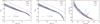 |
Fig. C.1 Mean value for the variance of the imaginary part of |
![Mathematical equation: $\[\delta \hat{\mathbf{p}}\]$](/articles/aa/full_html/2026/01/aa56491-25/aa56491-25-eq288.png)
![Mathematical equation: $\[\delta \hat{\mathbf{p}}\]$](/articles/aa/full_html/2026/01/aa56491-25/aa56491-25-eq289.png)
Appendix D Computing unbiased variances with Planck half-maps
Our methodology is based on the calculation of covariances of Planck residual maps. Residual maps Ri, ![Mathematical equation: $\[R_{i}^{P}\]$](/articles/aa/full_html/2026/01/aa56491-25/aa56491-25-eq290.png) and
and ![Mathematical equation: $\[R_{i}^{\psi}\]$](/articles/aa/full_html/2026/01/aa56491-25/aa56491-25-eq291.png) , as computed from Eqs. (18), (21) and (22) involve a combination of the complex polarized intensity maps Pi for channel i and P0 for the reference channel. In this section, we describe how to compute in practice variances of residual maps.
, as computed from Eqs. (18), (21) and (22) involve a combination of the complex polarized intensity maps Pi for channel i and P0 for the reference channel. In this section, we describe how to compute in practice variances of residual maps.
The variance ![Mathematical equation: $\[\mathbf{c}_{i i}^{\mathbf{P}}=\left\langle\mathbf{R}_{i} \mathbf{R}_{i}^{\star}\right\rangle\]$](/articles/aa/full_html/2026/01/aa56491-25/aa56491-25-eq292.png) being the mean value of a squared quantity, it will be biased by noise unless one uses the product of two uncorrelated versions of the same map
being the mean value of a squared quantity, it will be biased by noise unless one uses the product of two uncorrelated versions of the same map ![Mathematical equation: $\[\mathbf{P}_{i}^{\text {HM1}}\]$](/articles/aa/full_html/2026/01/aa56491-25/aa56491-25-eq293.png) and
and ![Mathematical equation: $\[\mathbf{P}_{i}^{\text {HM2}}\]$](/articles/aa/full_html/2026/01/aa56491-25/aa56491-25-eq294.png) called half-maps. From Eq. (18) we define the two complex residuals half-maps
called half-maps. From Eq. (18) we define the two complex residuals half-maps ![Mathematical equation: $\[\mathbf{R}_{i}^{\mathrm{HM} 1}\]$](/articles/aa/full_html/2026/01/aa56491-25/aa56491-25-eq295.png) and
and ![Mathematical equation: $\[\mathbf{R}_{i}^{\mathrm{HM} 2}\]$](/articles/aa/full_html/2026/01/aa56491-25/aa56491-25-eq296.png) for channel i by replacing the complex maps Pi and P0 by their corresponding half-maps, and the real map P0 by its unbiased10 estimate
for channel i by replacing the complex maps Pi and P0 by their corresponding half-maps, and the real map P0 by its unbiased10 estimate ![Mathematical equation: $\[\sqrt{\operatorname{Re}\left(\mathbf{P}_{0}^{\mathrm{HM} 1} \times\left(\mathbf{P}_{0}^{\mathrm{HM} 2}\right)^{\star}\right.}\]$](/articles/aa/full_html/2026/01/aa56491-25/aa56491-25-eq297.png) . The expression for the variance
. The expression for the variance ![Mathematical equation: $\[\mathbf{c}_{i i}^{\mathbf{P}}\]$](/articles/aa/full_html/2026/01/aa56491-25/aa56491-25-eq298.png) (Eq. (30)) then simply reads:
(Eq. (30)) then simply reads:
![Mathematical equation: $\[\mathbf{c}_{i i}^{\mathbf{P}}=\left\langle\mathbf{R}_i^{\mathrm{HM} 1} \mathbf{R}_i^{\star^{\mathrm{HM} 2}}\right\rangle.\]$](/articles/aa/full_html/2026/01/aa56491-25/aa56491-25-eq299.png) (D.1)
(D.1)
For i ≠ j, the covariance ![Mathematical equation: $\[\mathbf{c}_{i j}^{\mathbf{P}}=\left\langle\mathbf{R}_{i} \mathbf{R}_{j}^{\star}\right\rangle\]$](/articles/aa/full_html/2026/01/aa56491-25/aa56491-25-eq300.png) involves the product of maps with uncorrelated noise11. It is therefore possible to keep the full maps Pi and Pj in this calculation, but not for P0. We build two mixed residual maps
involves the product of maps with uncorrelated noise11. It is therefore possible to keep the full maps Pi and Pj in this calculation, but not for P0. We build two mixed residual maps ![Mathematical equation: $\[\mathbf{R}_{i}^{\mathrm{MX} 1}\]$](/articles/aa/full_html/2026/01/aa56491-25/aa56491-25-eq301.png) and
and ![Mathematical equation: $\[\mathbf{R}_{i}^{\mathrm{MX} 2}\]$](/articles/aa/full_html/2026/01/aa56491-25/aa56491-25-eq302.png) from Eq. (18) by keeping the full map Pi but still replacing the reference maps P0 by its corresponding half-map (the map P0, playing the role of a weight, remains the same). With these notations,
from Eq. (18) by keeping the full map Pi but still replacing the reference maps P0 by its corresponding half-map (the map P0, playing the role of a weight, remains the same). With these notations,
![Mathematical equation: $\[\mathbf{c}_{i j}^{\mathbf{P}}=\left\langle\mathbf{R}_i^{\mathrm{MX} 1} \mathbf{R}_j^{\star \mathrm{MX} 2}\right\rangle \quad \forall i \neq j.\]$](/articles/aa/full_html/2026/01/aa56491-25/aa56491-25-eq303.png) (D.2)
(D.2)
A small bias will remain in each component of the covariance matrix cP due to chance correlation, which we attempt to suppress by using simulations (see Sect. 4.3 and our discussion in Sect. 6). The same procedure is applied to compute the real covariance matrices ![Mathematical equation: $\[c_{i j}^{P}, c_{i j}^{\psi}\]$](/articles/aa/full_html/2026/01/aa56491-25/aa56491-25-eq304.png) and
and ![Mathematical equation: $\[c_{i j}^{\psi P}\]$](/articles/aa/full_html/2026/01/aa56491-25/aa56491-25-eq305.png) .
.
Appendix E Results with the Planck PR4 release
In this section, we present the results obtained by replacing Planck SRoll2 data by the Planck PR4 maps and NPIPE simulations, and compare them with those obtained with Planck SRoll2 data. Figures E.1, E.2, E.3 and Tables E.1 and E.2 present the results we obtain replacing the SRoll2 version of Planck data by the last official Planck release PR4. We remind the reader that all our calculated covariances are independent of any possible calibration error in the polarization data, either in amplitude or in phase (see Sect. 4.3), thereby facilitating the comparison between the properties of these two versions of Planck data.
The mean complex SED for PR4 (Fig. E.1, top left panel, black solid line) differs in angle from that of SRoll2 (green solid line) at 100 and 217 GHz, but not at 143 GHz. This reveals the distinct treatment of CO-contaminated channels between these two versions of Planck data. Predictions P2, P3, and P4 (Fig. E.1, top right panel) are verified using PR4, like for SRoll2. Inspection of polarization ratios cψ/cP (predictions P5 and P6, Fig. E.1, bottom left panel) lead to the same conclusions like for SRoll2. Like for SRoll2 prediction P7 (Fig. E.1, bottom right panel and Table E.2) is not verified for PR4, with a higher discrepancy than with SRoll2 owing to the smaller error bars from PR4.
The main difference between PR4 and SRoll2 arises in the level of correlation between residual maps (Table E.1) and in the spectral dependence of covariances (Fig. E.2). Table E.1 shows that prediction P1 is not verified with PR4, even for RP residual maps: the Pearson coefficient between residual maps is systematically lower with PR4 than with SRoll2 (owing to the larger error bars for SRoll2 these values remain compatible, however). Comparing PR4 and SRoll2 covariances in Fig. E.2, we see that cψ covariances are, within error bars, compatible. This is remarkable as the mean SEDs are different. This probably means that the main difference regarding polarization angles between these two version of Planck data lies in the mean complex SED, not in the fluctuations around this mean. Covariances cP are compatible, except for ![Mathematical equation: $\[c_{217 \times 217}^{P}\]$](/articles/aa/full_html/2026/01/aa56491-25/aa56491-25-eq306.png) for which the discrepancy by far exceeds uncertainties. The χ2 fits to the PR4 data are bad for our two scenarios (whether T or β fluctuate, hypothesis HM3). The covariances
for which the discrepancy by far exceeds uncertainties. The χ2 fits to the PR4 data are bad for our two scenarios (whether T or β fluctuate, hypothesis HM3). The covariances ![Mathematical equation: $\[c_{100 \times 100}^{\psi}\]$](/articles/aa/full_html/2026/01/aa56491-25/aa56491-25-eq307.png) and
and ![Mathematical equation: $\[c_{100 \times 100}^{P}\]$](/articles/aa/full_html/2026/01/aa56491-25/aa56491-25-eq308.png) clearly depart from the general trend. Removing them from the fitted values does not however improve the fit dramatically.
clearly depart from the general trend. Removing them from the fitted values does not however improve the fit dramatically.
Finally, the correlation between SEDs in polarization (PR4) and intensity (d1) in Fig. E.3 reveals a good level of correlation, but not as strong as with SRoll2 (Fig. 9). This is probably a consequence of the demonstration by Fig. E.2 that the fluctuations around the mean SED in PR4 do not follow a spectral behavior corresponding to fluctuations of β or T, unlike for d1 and SRoll2.
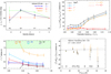 |
Fig. E.1 Same as Figs. 4, 5, 6 and 8, but for the Planck PR4 official release. To facilitate the comparison between PR4 and SRoll2 in the top left figure, the mean SRoll2 debiased SED is overplotted in green. |
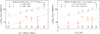 |
Fig. E.2 Same as Fig. 7, but for the Planck PR4 official release. To facilitate comparison between PR4 and SRoll2, data with errors bars for SRoll2 are overplotted with no symbols. |
Appendix F Using other PYSM 3 dust models for debiasing
Figure F.1 presents how our estimate for the bias produced on covariances by CMB and noise and systematics depends on the dust model chosen to compute this estimate. From Eq. (40) we compute, for each model and for each member of the covariance matrix, the mean bias ![Mathematical equation: $\[c_{\text {bias}} \equiv \frac{1}{N_{\text {sims}}} {\sum}_{k=1}^{N_{\text {sims}}} c_{\text {bias}}(k)\]$](/articles/aa/full_html/2026/01/aa56491-25/aa56491-25-eq313.png) together with its uncertainty (the standard deviation of cbias(k)). We compare the amplitude and error bars of cbias for the three PYSM 3 dust models d1, d10 and d12, for cP (left) and cψ (right). Although the covariances of models strongly differ, all biases estimated are compatible for all couple of channels, within the uncertainties computed from the 200 SRoll2 simulations.
together with its uncertainty (the standard deviation of cbias(k)). We compare the amplitude and error bars of cbias for the three PYSM 3 dust models d1, d10 and d12, for cP (left) and cψ (right). Although the covariances of models strongly differ, all biases estimated are compatible for all couple of channels, within the uncertainties computed from the 200 SRoll2 simulations.
Figure F.2 presents the mean SED derived from Planck SRoll2 data using the dust models d10 (left) and d12 (right) to debias covariances from CMB, noise and systematics. There is no significant difference with the one obtained with model d1 (Fig. 4).
Figure F.3, like Fig. 6, presents how the ratio cψ/cP vary with fsky when using dust models d10 (left) and d12 (right) to debias covariances from CMB, noise and systematics. Our conclusions remain the same.
Figure F.4 presents the correlation of Planck SRoll2 polarization maps residuals with dust models d10 (left) and d12 (right). Variances are for d10 (based on GNILC maps) around 4 times the one found our reference model d1 (based on Commander maps). For d12, this is a factor 7. Note that in our analysis the values of variances are dominated by fluctuations in the Galactic plane owing to the weight ![Mathematical equation: $\[P_{0}^{2}\]$](/articles/aa/full_html/2026/01/aa56491-25/aa56491-25-eq314.png) for the calculation of covariances (see Eq. (25)). Nevertheless, the correlation of polarization data with d10 in residual maps is similar to the one obtained in Fig. 9 for the d1 dust model. SED fluctuations present in the d12 dust model anticorrelates with polarization data. The reason for this behavior is unknown.
for the calculation of covariances (see Eq. (25)). Nevertheless, the correlation of polarization data with d10 in residual maps is similar to the one obtained in Fig. 9 for the d1 dust model. SED fluctuations present in the d12 dust model anticorrelates with polarization data. The reason for this behavior is unknown.
Figure F.5, like Fig. 7, presents the spectral dependence of covariances with the product of first-order spectral gradients coefficients ai,1aj,1, for β (left) and T (right), using the d10 (top) and d12 (bottom) dust models for debiasing.
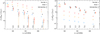 |
Fig. F.1 Effect of the dust model on the amplitude of bias and error-bars estimates for cP (left) and cψ (right). |
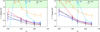 |
Fig. F.3 Same as Fig. 6 for the d10 (left) and d12 (right) PYSM 3 dust models. The hashed region represents forbidden values according to P5. |
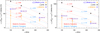 |
Fig. F.4 Same as Fig. 9, but for d10 (left) and d12 (right) PYSM 3 dust models. Both models are dominated by fluctuations of β and have too much variance with respect to polarization data (by a factor ~4 and ~7, respectively), for our 97.3% mask dominated by the Galactic plane. |
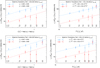 |
Fig. F.5 Comparison of SRoll2 data with the predictions of dust model d10 (top) and d12 (bottom), for cP (blue) and cψ (red), for pure β fluctuations (left) and pure T fluctuations (right). |
All Tables
All Figures
|
Fig. 1 Values of |
| In the text | |
|
Fig. 2 Rotation of the SED in the complex plane for a sum of seven MBB SEDs with distinct spectral indices drawn from a Gaussian distribution with mean 1.5 and standard deviation 0.1 (red), or with temperatures drawn from a Gaussian distribution with mean 20 K and standard deviation 5 K (blue). The 3D orientation of the magnetic field is a random realization of the turbulent magnetic field inspired by Planck Collaboration Int. XLVIII (2016). The dashed lines indicate frequencies from 40 to 400 GHz, and the four colored points represent the Planck HFI bands. |
| In the text | |
|
Fig. 3 HEALPix masks with growing fsky (Nside = 32): 85% (dark blue), 90% (light blue), 92% (green), 95% (orange), and 97.3% (brown). The 97.3% mask additionally excludes the inner Galactic plane within 3 degrees of latitude and pixels within 4 degrees of the Crab pulsar (gray). |
| In the text | |
|
Fig. 4 Mean complex polarized SED |
| In the text | |
|
Fig. 5 Test of predictions P2, P3, and P4: dependence on the observed polarization fraction p0 = P0/I0 at 353 GHz of the variances Re cP, cP, cψ, and cε computed at 217 GHz. Our models for cε (P2) and cψ (P3) are overplotted as dotted orange and red lines, respectively, using the mean value of the slope derived from these equations, multiplied by |
| In the text | |
|
Fig. 6 Test of predictions P5 and P6 as a function of fsky. The hashed region represents forbidden values according to P5. |
| In the text | |
|
Fig. 7 Comparison of SRoll2 data with the predictions of our model for cP (blue) and cψ (red), for pure β fluctuations (top), and pure T fluctuations (bottom). |
| In the text | |
|
Fig. 8 Covariances |
| In the text | |
|
Fig. 9 Comparison of the spectral dependence of covariances cε from SRoll2 data, cP for the dust model d1, and cP for the cross-product of SRoll2 and d1. The Pearson correlation coefficient ρ(d1, SR) is indicated (purple). Predictions for models with T or β fluctuations are overplotted. |
| In the text | |
|
Fig. C.1 Mean value for the variance of the imaginary part of |
| In the text | |
|
Fig. E.1 Same as Figs. 4, 5, 6 and 8, but for the Planck PR4 official release. To facilitate the comparison between PR4 and SRoll2 in the top left figure, the mean SRoll2 debiased SED is overplotted in green. |
| In the text | |
|
Fig. E.2 Same as Fig. 7, but for the Planck PR4 official release. To facilitate comparison between PR4 and SRoll2, data with errors bars for SRoll2 are overplotted with no symbols. |
| In the text | |
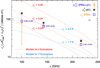 |
Fig. E.3 Same as Fig. 9, but for the Planck PR4 official release. |
| In the text | |
|
Fig. F.1 Effect of the dust model on the amplitude of bias and error-bars estimates for cP (left) and cψ (right). |
| In the text | |
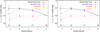 |
Fig. F.2 Same as Fig. 4, but for d10 (left) and d12 (right) PYSM 3 dust models. |
| In the text | |
|
Fig. F.3 Same as Fig. 6 for the d10 (left) and d12 (right) PYSM 3 dust models. The hashed region represents forbidden values according to P5. |
| In the text | |
|
Fig. F.4 Same as Fig. 9, but for d10 (left) and d12 (right) PYSM 3 dust models. Both models are dominated by fluctuations of β and have too much variance with respect to polarization data (by a factor ~4 and ~7, respectively), for our 97.3% mask dominated by the Galactic plane. |
| In the text | |
|
Fig. F.5 Comparison of SRoll2 data with the predictions of dust model d10 (top) and d12 (bottom), for cP (blue) and cψ (red), for pure β fluctuations (left) and pure T fluctuations (right). |
| In the text | |
Current usage metrics show cumulative count of Article Views (full-text article views including HTML views, PDF and ePub downloads, according to the available data) and Abstracts Views on Vision4Press platform.
Data correspond to usage on the plateform after 2015. The current usage metrics is available 48-96 hours after online publication and is updated daily on week days.
Initial download of the metrics may take a while.