| Issue |
A&A
Volume 705, January 2026
|
|
|---|---|---|
| Article Number | A133 | |
| Number of page(s) | 11 | |
| Section | The Sun and the Heliosphere | |
| DOI | https://doi.org/10.1051/0004-6361/202557052 | |
| Published online | 13 January 2026 | |
Connecting solar wind turbulence to plasma parameters at L1 using multi-spacecraft coherence
1
Cooperative Institute for Research in Environmental Sciences, University of Colorado Boulder Boulder CO, USA
2
Princeton University Princeton NJ, USA
3
National Centers for Environmental Information, National Oceanographic and Atmospheric Administration Boulder CO, USA
★ Corresponding author: This email address is being protected from spambots. You need JavaScript enabled to view it.
Received:
31
August
2025
Accepted:
2
December
2025
Abstract
Context. Solar wind propagation behavior has significant implications for solar wind forecasting and measurements. Variability in coherence and plasma turbulence under different plasma conditions is important for cross-satellite comparisons. Forecasting also depends on whether upstream measurements remain valid at the magnetosphere.
Aims. We used computational methods to analyze magnetic coherence and connections to plasma parameters, utilizing multi-decade ACE and Wind measurements to capture turbulence behavior across a wide range of spatial separations and solar cycle phases.
Methods. The measurements were separated into three frequency ranges within the inertial range of solar wind turbulence: in periods of 1–2.5 min, 2.5–10 min, and 10–30 min. We assessed the coherence in each frequency band using time-lagged cross-correlations and applied a clustering algorithm to identify connections between coherence and plasma parameters (velocity, proton density, flow pressure). We performed this analysis in the radial, nonradial, and total directions.
Results. We used a k-means clustering algorithm to find that higher coherence in all cases is associated with smaller variance in plasma parameters. Taking this into consideration, we find a trivial association with the satellite separation or solar cycle phase. Small variations in dynamic pressure and velocity appear to be the best indicators of high coherence at these high-frequency inertial scales. Identifying connections between turbulence and plasma parameters could improve our understanding of the underlying physical processes. This information will also be vital for instrument calibration on future missions such as the Space Weather Follow On L1 (SWFO-L1).
Key words: plasmas / turbulence / methods: statistical / Sun: heliosphere / Sun: magnetic fields / solar wind
© The Authors 2026
 Open Access article, published by EDP Sciences, under the terms of the Creative Commons Attribution License (https://creativecommons.org/licenses/by/4.0), which permits unrestricted use, distribution, and reproduction in any medium, provided the original work is properly cited.
This article is published in open access under the Subscribe to Open model. This email address is being protected from spambots. You need JavaScript enabled to view it. to support open access publication.
1. Introduction
The solar wind is a constant flow of magnetized plasma propagating from the solar corona throughout the Solar System (Verscharen et al. 2019). It serves as the medium through which disturbances from the sun propagate to the Earth, while solar wind turbulence can also affect high-energy particle acceleration and cosmic ray behavior (Bruno & Carbone 2013; Inceoglu et al. 2022). Furthermore, geomagnetic activity can be driven by certain solar wind conditions (Schwenn 2006; Inceoglu & Loto’aniu 2023; Loto’aniu & Inceoglu 2024; Inceoglu & Loto’aniu 2025) and, given the potentially destructive nature of such disturbances (Pulkkinen 2007), upstream solar wind monitors play an important role in understanding and forecasting solar wind and magnetospheric dynamics (Burkholder et al. 2020; Horne et al. 2013). Such spacecraft include NASA’s Advanced Composition Explorer (ACE; Stone et al. 1998) and Wind (Acuña et al. 1995) spacecraft, which are located at the first Lagrange point (L1). Given that L1 is 1.5 million kilometers from the Earth toward the Sun, the question arises as to whether measurements of solar wind parameters made at L1 remain valid at the magnetosphere. Overall, it depends on the level of coherence (i.e., the spatiotemporal extent to which turbulent structures can propagate relatively unchanged) in the solar wind at L1 (Matsui et al. 2002).
With the growing constellation of satellites at L1, the question of coherence also arises in the task of satellite instrument calibration and validation via cross-satellite comparisons. Measurements taken onboard the National Oceanic and Atmospheric Administration (NOAA) Deep Space Climate Observatory (DSCOVR, Burt & Smith 2012) were calibrated via cross-satellite comparisons and a similar procedure is planned for the upcoming NOAA Space Weather Follow On L1 (SWFO-L1). Given that the validity of cross-satellite measurement comparisons is inherently determined by coherence, identifying ideal orbital and plasma conditions for satellite cross-comparison remains an active area of research (Loto’aniu et al. 2022).
For decades, solar wind coherence in magnetic field measurements has been investigated in relation to satellite separation (Russell et al. 1980; Crooker et al. 1982; Matsui et al. 2002; Matthaeus et al. 2005; Wicks et al. 2009; Matthaeus et al. 2016; Ragot 2022). Such prior works have established that the coherence of magnetic field turbulence tends to decrease with increasing spacecraft separation. However, there is also consistent recognition that spacecraft separation is not sufficient to capture all trends in coherence (Chang & Nishida 1973; Loto’aniu et al. 2022). This has been addressed in the context of other potential factors, including the frequency of magnetic field fluctuations. For example, Matsui et al. (2002) found that greater coherence is generally associated with lower-frequency fluctuations, but noting that further investigation into coherence in relation to plasma conditions is necessary. They also found that using time-domain and frequency-domain approaches to turbulence scale analysis yield similar results. Matsui et al. (2002) also performed this analysis in different spatial orientations. They found that coherence levels fall off significantly faster perpendicular to the Earth-Sun line than parallel to it. However, high variability and unclear associations between orientation and coherence remain prominent (Wicks et al. 2009). There has also been significant interest in connecting coherence with the solar cycle. Collier et al. (1998), King & Papitashvili (2005), and Wicks et al. (2009) all found that coherence generally increases during the solar maximum. However, disagreement remains over which variables show association with solar activity (total interplanetary magnetic field (IMF) magnitude, IMF components, plasma conditions, etc.). The final variable that is generally considered in relation to solar wind turbulence scales is the plasma velocity. While some works have found higher coherence to be linked to slower solar wind conditions, the results are often not very robust and require more detailed investigation (Crooker et al. 1982; Wicks et al. 2009; Matthaeus et al. 2016).
In this study, we use time-lagged cross correlations between ACE and Wind magnetic field measurements to assess plasma turbulence scales within different frequency bands. We test significantly higher frequencies than previous works (Matsui et al. 2002; Wicks et al. 2009), probing deeper into the inertial range of solar wind turbulence (Goldstein & Roberts 1999). In addition, we use a k-means clustering algorithm to test for connections between turbulence scales and fundamental plasma parameters, solar cycle phases, and satellite separation. To our knowledge, this is the first time that the coherence of solar wind turbulence has been directly connected to plasma conditions at L1.
The rest of this paper is organized as follows. Section 2 describes the data and preprocessing steps, the time-lagged cross-correlation method, and the clustering algorithm. Section 3 presents our results and Section 4 draws comparisons to prior work and discusses physical and practical implications.
2. Methods
2.1. Data and preprocessing
We used solar cycle 24 for our analysis of coherence across solar cycle phases and selected two years of data for each solar cycle phase: increasing (2010–2011), maximum (2012–2013), decreasing (2015–2016), and minimum (2018–2019). The ACE and Wind data were obtained from NASA’s Coordinated Data Analysis Web (CDAWeb)1. We used spacecraft position and magnetic field data from both satellites, as well as plasma velocity and proton density data from Wind. We did not use ACE plasma velocity or density data due to issues with low cadences and missing data intervals. All vector quantities (position, magnetic field, and plasma velocity) are in the Geocentric Solar Ecliptic (GSE) coordinate system. The data products selected to maximize data quality and minimize gaps are displayed in Table 1, along with a list of the variable extracted and measurement cadence for each data product.
Summary of data products used in this study.
Magnetic field measurements were unified to a 3 second cadence via mean resampling, while all other parameters were unified to a 1 minute cadence by linearly interpolating between the data points. We would like to note that they are interpolated raw data values and not averages. This unification method ensured that we had access to the highest available resolution for each quantity.
The plasma flow pressure (FP) in nPa can be calculated using Equation (1),
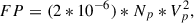 (1)
(1)
where Np is proton density in cm−3 and Vp is the proton speed in km/s. This formula is used to calculate flow pressure for NASA’s OMNIWeb data products2 and it was validated by exactly reproducing OMNIWeb flow pressure time-series data.
Magnetic field, plasma velocity, proton density, and flow pressure measurements were separated into fundamental frequency bands using a 4th-order Butterworth bandpass filter. The highest frequency band is the continuous pulsation 4 (Pc4) range, which includes fluctuations with periods from approximately 1–2.5 min. Given that the Nyquist limit for this band would be given in periods of 30 seconds, our 3 second data cadence allows us to avoid aliasing and any frequency biases. We also extract the Pc5 range, which includes periods from 2.5 to 10 min. The lowest frequency band includes fluctuations with periods from 10 to 30 min. This range overlaps with the lowest-frequency domains examined in prior studies (Matsui et al. 2002) and we extended our analysis far into the inertial range to the highest frequencies permitted by the satellite data cadences. This permits a novel analysis of turbulence scales within the inertial range of the solar wind. We followed the conventional magnetospheric frequency band ranges and nomenclature, as outlined in Jacobs et al. (1964), noting that it has been suggested that pulsations are driven directly by waves in the solar wind, as seen in proton density and flow pressure (Kepko et al. 2002). To corroborate this frequency range choice, we performed identical coherence analysis using equal-width ranges (e.g., a range of a factor of 3 captured by each bin). We found no meaningful differences and, thus, we adopt the Pc4/5 nomenclature given its physical relevance as well as its convenience.
2.2. Time-lagged cross-correlation
Solar wind coherence for a given time interval is calculated via a novel sliding window cross-correlation method by which we obtain the time lag between the two satellites’ magnetic field measurements as well as the correlation between the two signals at that time. The time lag between signals is the temporal delay between when each satellite detects a given feature (i.e., the solar wind propagation time from one satellite to the other). Here, we present an illustrative example of our cross-correlation method for Pc4 fluctuations in the GSE x-direction (radial) on May 24, 2011 at 2:36 UTC (i.e., during the increasing phase of solar cycle 24), shown in Figure 1.
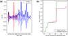 |
Fig. 1. Illustrative example of our time-lagged cross-correlation method. The two satellites’ magnetic field time series are shown in panel (a) starting on May 24th, 2011 at 2:36 UTC. The magnetic field time series recorded by the satellite closer to the sun (Wind; Satellite 1) is slid across the second satellite’s measurements, calculating the correlation between the two signals at each point. Panel (a) also includes the signal envelopes for each time series for ease of visual comparison (darker-colored lines). Panel (b) shows the maximum correlation recorded up to that point for each time delay, for both the magnetic field time-series (pink) and signal envelopes (green). We define the time lag between signals to be where there is the greatest improvement in correlation between the signals, and the coherence to be the correlation at that point (in this case, a correlation of 0.595 at a lag of 22 min). |
First, a 30-minute period of data was identified for which Wind was closer to the sun (red line in Figure 1a). Changing the window length of 30 minutes would inherently affect the correlation values. However, it would be systematic and, thus, it would not affect investigations of relative coherence or associations between variables, which are the primary goals of this work. We then extracted a longer time series recorded at ACE, (blue line in Figure 1a). We defined this additional length to be (30 + 4 * T) minutes, where T represents the longest period in this frequency band. This window length ensures that the first signal is slid at least its own length and we captured at least five periods at the longest period tested (30 minutes). We later show that this method is insensitive with respect to how far the window is slid. The first signal is slid along the second signal point-by-point and a Pearson correlation coefficient between the two bandpass-filtered signals can be calculated via Equation (2),
 (2)
(2)
where Cij represents the covariance matrix element of the two variables xi and xj.
Figure 1b shows the maximum correlation coefficient recorded so far, while the first signal is slid along the second. This plot illustrates why it is not valid to simply take the maximum correlation. Visually, there is an approximately 20-minute time lag between the main wave-form recorded at each satellite. This is especially clear from the extrema of the amplitudes (see signal envelopes) and decay of the signal amplitudes from the −Bx spike. In spite of this, a slightly higher correlation was achieved much later at a 38-minute lag, as seen in the second step in the pink curve in Figure 1b. Thus, we defined the time lag between the two signals to be where there is the greatest improvement in correlation (i.e., the tallest step in Figure 1b). This is confirmed in the lagged cross-correlation of the envelopes (green), which shows a clear peak at 22 minutes. This method is hereafter referred to as the max-step correlation function. The only observed exception to this method is when there is significant improvement at unrealistically small time lags. Thus, we cut off the smallest time lags based on the radial satellite separation (assumed to be constant over 30-minute window) and plasma velocity. We calculated the mean and standard deviation of the plasma velocity in the 30-minute window and used it to cut off the time series three standard deviations below the theoretical time lag. This ensures that all possible time lags (including zero) are considered only when the satellites are radially close together. This method of calculating the time-lagged cross correlation between two signals is insensitive to how far the window is slid forward. In other words, a simple maximum-correlation approach would be more prone to significant changes based on a handful of data points that have been included or not included in the window. Thus, the max-step method removes potential biases introduced by manually entered window lengths or slide domains. For this illustrative example, a correlation coefficient of 0.595 was recorded with a 22 minute lag between the signals, matching the time delay visually clear in the signals. To validate this method, we performed a visual examination of six months of random intervals. We note that in cases where the absolute maximum correlation matches the correct time lag, we did not observe any additional jumps in the correlation. Thus, our method was able to correctly identify the proper time lag.
For an additional validation of the max-step method, we created synthetic random-noise sinusoidal signals with known time lags. We tested both taking the absolute maximum of the signal cross-correlation and taking the max step. As mentioned above, we found that the accuracy of the max-step function is completely independent of the sliding window domain, while the absolute-maximum approach is not. Specifically, by adjusting the sliding window domain, the absolute-max version can lose up to 30% accuracy, while the max-step version is completely insensitive across multiple orders of magnitude in input parameters. This empirically reflects the resistance of our max-step method to manually set parameters. Thus, we used this method to determine both the time lag between the two satellites and the point-by-point correlation at that time. Calculating the time lag separately was also necessary because it does not generally necessarily follow a simple relationship with plasma velocity and spacecraft separation (Wicks et al. 2009), potentially due to wave propagation effects.
For the large-scale statistical purpose of this study, we applied this max-step correlation function to 25 000 random intervals per solar cycle phase. This yields a total of 100 000 data points over all four phases. Expanding on prior work examining coherence in radial versus nonradial directions (Matsui et al. 2002), we perform magnetic coherence analysis in the GSE x-, y-, and z-directions, as well as using total separation (four direction cases). We also considered three possible frequency bands (Pc4, Pc5, and 10–30 min periods), yielding 12 cases in total.
2.3. Clustering
For each random 30-minute sliding window, in addition to the satellite separation, we note the standard deviation of the plasma velocity component(s), proton density, and flow pressure over the interval recorded by Wind. We would like to emphasize that these are calculated from the highpass-filtered data, resulting in significantly smaller values than the raw measurements. Given these parameters define the local dynamics of the solar wind plasma, we utilized the standard deviations of plasma velocity, proton density, and flow pressure as indicators of variations in plasma conditions and potential effects on coherence scales. Vector quantities (separation and velocity) are separated into the components corresponding to the specific orientation being considered. For example, in the radial (GSE x-direction) case, we considered the radial magnetic field, radial satellite separation, and radial plasma velocity. For each of the 12 frequency-direction cases, the final output of this process is a dataset of 100 000 coherence values, each associated with a solar cycle phase, satellite separation, time lag, and standard deviations of the plasma velocity, proton density, and flow pressure within the defined sliding window. We would like to note that although the spacecraft do not spend equal periods of time at all physical separations, our statistical approach is insensitive to this because we are only seeking to identify what physical conditions are associated with high coherence, which we do not expect to be affected by the variable separation distribution.
To identify potential associations between coherence levels and plasma parameters, we used a form of the popular k-means clustering algorithm. K-means clustering algorithms iteratively attempt to minimize the sum of squared errors, also known as cluster inertia, within each cluster (MacQueen 1967). We used a variant of this algorithm called the k-means++ algorithm, which has the same fundamental mechanism but increases performance by seeding the traditional k-means algorithm such that clusters are more distinct from each other (Arthur & Vassilvitskii 2007). This algorithm requires that the ideal number of clusters is specified a priori. We determined this first by using elbow plots. Plotting the within-cluster inertia as a function of number of clusters, k, we can visually determine the point at which adding additional clusters ceases to make meaningful performance improvements. This method was corroborated through the use of an agglomerative hierarchical clustering technique, where smaller clusters are iteratively merged until the entire sample belongs to one cluster. We use Ward’s method (Ward 1963), where clusters were merged based on minimizing the resultant sum of squared errors. The result of this algorithm can be plotted as a dendrogram, which displays the clusters formed in the agglomerative process and the resulting similarity between clusters at each iteration, as calculated via the Euclidean distance metric. The ideal number of clusters is visually selected to achieve a desired level of similarity within each cluster (Murtagh & Contreras 2012). By combining the results of the elbow plot and the agglomerative clustering algorithm, we determined the ideal number of clusters to initialize the k-means++ algorithm (hereafter, simply referred to as k-means). We did this for each of the 12 cases and the final model output consists of a statistical association between magnetic coherence, satellite separation, time lag, and plasma parameter variability. We note that we did not include solar cycle phase information in the clustering algorithm, as the inherent four discrete cases (increasing, maximum, decreasing, minimum) bias the clustering algorithm and outweigh any potential connections between other variables.
3. Results
Overall coherence over space and time is analyzed via heatmap plots. Figure 2 shows heatmap plots for the GSE x (radial) direction, with each frequency domain (Pc4, Pc5, 10–30 min) as a panel. In each plot, the x-axis represents spatial satellite separation and the y-axis represents temporal signal separation (time lag), as determined by the max-step correlation function described in Section 2.2. We would like to note that the diagonal cutoff region at the bottom of each plot is the result of cutting off unrealistically small time lags in the max-step correlation function (see Section 2.2). Similar cutoffs in the heatmaps for the GSE y and z directions are also the result of orbital geometry and removing unrealistically small lags. The large-scale statistical nature of this plot (including observations across vastly different plasma conditions and cycle phases) makes it difficult to identify detailed associations. However, on a global level, the primary trend which is immediately evident is that the highest correlations (darkest red) are observed in fluctuations with periods between 10 and 30 minutes. The next highest correlations are seen in the Pc5 frequency band (periods between 2.5 and 10 minutes). Finally, the lowest coherence is seen in the highest frequency band (Pc4), with periods between 1 and 2.5 minutes. The orbital geometries of the satellites result in a greater number of observations at larger separations (see Section 2.3 for detailed discussion). We perform this heatmap analysis in the GSE y-, z-, and total directions as well (Figures S1, S2, S3). In all cases, we observe the same key features as outlined above. We do not observe any clear or well-constrained falloff in coherence over distance at these frequency scales (1–30 min periods); instead, we found an extremely large range in coherence values for any given distance. This is in line with prior coherence results presented by Wicks et al. (2009) and is reflected in the heatmap plots, which do not show a clear falloff with distance.
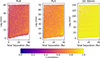 |
Fig. 2. Spatiotemporal heatmaps of radial ACE-Wind magnetic coherence observed at L1. Each panel corresponds to fluctuations within a given frequency range of magnetic field fluctuations: Pc4 (1–2.5 min), Pc5 (2.5–10 min periods), and 10–30 min periods. For each plot, the x-axis represents radial spacecraft separation and the y-axis represents the time lag between signals recorded at each satellite. The color intensity of each point represents the coherence observed at that particular temporal and spatial lag, as determined by our max-step correlation function. Each plot contains 10 000 observations across various plasma conditions and solar cycle phases, so opacity is adjusted to emphasize higher concentrations of high-coherence observations. |
To further investigate associations between coherence, satellite separation, and plasma conditions within these frequency bands, we use a k-means clustering algorithm. Ideal cluster numbers are determined via elbow plots and agglomerative clustering dendrograms, which are standard methods of clustering algorithm optimization (Syakur et al. 2018; Dash et al. 2003). The top row of Figure 3 displays both of these plots for fluctuations in the Pc4 frequency range (1–2.5 min periods) in the GSE x-direction (radial). Figure 3a shows within-cluster error for a domain of 1–10 clusters, and there is a slight elbow at k = 3 (i.e., beyond k = 3, additional clusters visually cease to make meaningful error reductions). The dendrogram (Figure 3b) also appears to show three primary clusters and, thus, we performed the k-means clustering with three clusters. The output of the k-means clustering algorithm is displayed in a parallel plot, which shows the associations between variables within each cluster (Figure 3c). The x-axis of Figure 3c shows each of the variables considered in clustering: Pearson r value (as determined by the max-step correlation function), standard deviations of velocity, proton density, and flow pressure over the interval, and spatial satellite separation. We also included time lag between signals in the clustering algorithm, because it is observed to not follow a simple correlation with satellite separation and plasma velocity, as found in prior work (Matsui et al. 2002). With this information included, the algorithm simply identifies that smaller time lags are generally associated with smaller satellite separations, as expected, so the time lag results are not shown here.
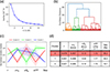 |
Fig. 3. Clustering results for fluctuations in the Pc4 range (1–2.5 min periods). Panel (a) shows an elbow plot, in which within-cluster error is displayed as a function of cluster number. Panel (b) displays the agglomerative clustering dendrogram, in which Euclidean distance indicates the similarity between clusters. We selected three main clusters. Panel (c) is a parallel plot of the clustering results. Within each of the three clusters, the median of each variable is calculated and plotted on a normalized scale (the displayed values are not the actual values), along with a statistical error margin defined by the standard error. Each colored line represents a cluster and displays the defining characteristics of each cluster. Panel (d) shows the non-normalized values plotted in the parallel plot, with the cluster with highest median coherence highlighted in red. Here, r represents the cross-correlation, σvx represents the median standard deviation of the plasma velocity in the x-direction, σNp represents the median s.d. of the proton density, σFP is the median s.d. of the flow pressure, and Sep. represents the median satellite separation for each cluster. |
The y-axis of Figure 3c shows the median value of each variable within each cluster for Pc4 fluctuations in the GSE x-direction, normalized between 0 and 1 for ease of visual comparison. This means that the values shown on the y-axis, for example, cluster number 2 (shown in blue), having a median correlation of zero, are not the real values. It simply indicates that cluster number 2 has the lowest median correlation of all three clusters. The non-normalized values (i.e., actual median values) are displayed in Figure 3d. The cluster with the highest median correlation (highest coherence) is highlighted in red. Together, the parallel plot and the data table display the associations between variables identified by the algorithm. Each colored line on the parallel plot represents one cluster and corresponds to a row in the data table. To assess the statistical significance of the clustering output, we display each value with an error bound defined by the standard error. Cluster number 0 has the highest median coherence with an r value of 0.476, which is approximately 13% higher than that for cluster 2 (the lowest median correlation). Cluster number 0 also is shown to have the lowest standard deviation of proton velocity and flow pressure. Both of these associations are statistically significant, given the full range of error lies outside of the standard error bounds of the other clusters. Cluster number 0 (highest median correlation) also has the second-highest median satellite separation of 30.2 Earth radii (Re), while cluster number 2 (lowest median correlation) has the smallest median separation.
We conducted the same clustering analysis for Pc4 fluctuation coherence in the total separation direction, considering all three components simultaneously. We found three main clusters (Figure 4a,b). The highest median correlation of 0.444 is linked to the lowest median standard deviation of plasma velocity and flow pressure (Figure 4c,d).
Figure 5 displays our GSE-x results for fluctuations in the Pc5 frequency range, corresponding to periods between 2.5 and 10 minutes. The elbow plot shows an “elbow” in three clusters and the dendrogram plot again shows an ideal k value (cluster number) of 3, which we use to achieve the k-means output in the bottom row of the figure. The red line represents the cluster with the highest median correlation of 0.621. Notably, this value is 30% higher than the highest median correlation in the Pc4 case, which was 0.476. This aligns with the overall coherence data displayed in Figure 2, which shows significantly lower coherence in the Pc4 case. The parallel plot shows that in this case, the highest correlations are associated with the smallest standard deviation of plasma velocity and flow pressure.
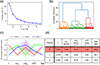 |
Fig. 5. Same as in Figure 3, but for Pc5 frequency range (2.5–10 min periods) in the GSE x-direction. |
Just as in the Pc4 case, we perform identical clustering analysis for the total direction. We identified three clusters, displaying a maximum correlation median of 0.583. This cluster is characterized by minimum values of plasma velocity and flow pressure standard deviation (Figure 6).
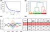 |
Fig. 6. Same as in Figure 3, but for fluctuations in the Pc5 frequency range (periods 2.5–10 min) and considering all three GSE components (total separation). |
Figure 7 displays clustering results for GSE-x fluctuations in the lowest frequency band tested (periods between 10 and 30 minutes). In this case, the elbow plot (Figure 7a) displays an ideal cluster number k = 3. The dendrogram plot shows three primary clusters, which we chose as the input for the final k-means clustering algorithm. The highest median correlation is 0.953, aligning with the heatmap plots of Figure 2, which show the highest overall coherence in the 10–30 min period band when compared to Pc4 and Pc5 fluctuations. From the parallel plot, we also observe that high correlations are associated with the smallest median standard deviation of plasma velocity.
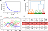 |
Fig. 7. Same as in Figure 3, but for fluctuations with periods between 10 and 30 minutes in the GSE-x direction. |
In the total direction, we again identified three clusters (Figure 8a,b). The maximum median correlation of 0.869 is associated with the minimum median standard deviations in plasma velocity and flow pressure (Figure 8c,d).
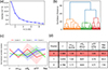 |
Fig. 8. Same as in Figure 3, but for fluctuations with periods ranging from 10 to 30 minutes and considering all three GSE components (total separation). |
In total, we performed clustering analysis for 12 cases: 3 frequency bands for fluctuations in 4 possible directions (3 coordinate directions plus total separation). We note that we display the radial (x) and total (x, y, and z together) results only, as the other cases (y and z) are highly similar and included in our overall analysis (see below). In each case, the clustering algorithm identifies distinct groups of observations, each characterized in terms of the variables considered: coherence (as measured by the max-step correlation function), satellite separation, and standard deviation of plasma velocity, proton density, and flow pressure. Table 2 displays a summary of these results. For all 12 cases, low standard deviations in plasma velocity, proton density, and/or flow pressure are associated with maximum coherence. In 9 out of 12 cases is there at least one characterizing minimum that lies within the standard error of another cluster (asterisk). However, in only 2 out of 12 cases are all of the characterizing minima within the standard error of another cluster. This means that in 10 out of 12 cases, the clustering results permit us to identify a statistically meaningful plasma parameter association, corroborating the robustness of our results. To verify the stability of these results, we have repeated this analysis with a range of sample sizes, extending down to 2500 intervals per solar phase. We find that the clustering associations stabilize above 10 000 intervals per phase.
Summary of clustering results for all 12 cases considered (3 frequency bands and 4 directions).
4. Discussion and conclusions
4.1. Overall coherence
Previous studies have found that overall coherence of turbulent structures generally appears to fall off with increasing fluctuation frequency. For example, Matsui et al. (2002) decomposed magnetic field signals into their Fourier components to assess coherence in different frequency domains. They found that high coherence is achieved for fluctuations with periods of 256 and 512 minutes, and coherence drops off for fluctuations below T = 128 minutes. The authors test frequencies down to T = 16 minutes. Wicks et al. (2009) also examined the effects of fluctuation frequency on coherence, utilizing two time windows: 200 minutes and 960 minutes. The first window focuses on the inertial range of solar wind turbulence, which includes timescales on the order of 10 seconds to multiple hours (Goldstein & Roberts 1999), while the second window focuses on large-scale solar wind structures. Wicks et al. (2009) found that the coherence falls off with increasing satellite separation more quickly for the shorter time window. In this study, we utilized a much shorter time window of only 30 minutes and with fluctuations periods ranging from 30 down to 1 minute, testing further into the inertial scale of solar wind turbulence than previous studies. As seen in Figure 2, coherence clearly increases with period, agreeing with the overall result of prior studies.
We also find that there is an extremely large range in coherence values at any given distance (this is true even at much larger timescales; see Wicks et al. 2009). Thus, other factors must be considered, as discussed in the next section.
4.2. Plasma parameter dependence
It can be seen from Table 2 that for all 12 cases, the highest median coherence is linked to low median values of standard deviations in plasma velocity, proton density, flow pressure, or some combination thereof. This means that small variance in plasma parameters over the 30-minute data interval is the best indicator of highly coherent turbulent structures on the frequency scales examined in the study. Physically, this can be interpreted as evidence that turbulent magnetic structures in the solar wind are significantly more likely to propagate without disruption or significant change when plasma conditions are calm (i.e., there are no major fluctuations in pressure, density, or velocity). Most notably, satellite separation was a worse predictor in the majority of cases across the Pc4, Pc5, and 10–30 min period bands. In fact, it can be seen from the parallel plots in Section 3 that in many cases, the cluster with the highest median coherence also had maximum or near-maximum median satellite separation. This means that even with near-maximum spacecraft separation, if plasma conditions are calm, the median coherence is maximized. To the best of our knowledge, previous studies using ACE and Wind magnetic field data to calculate coherence have all found coherence to fall off with increasing satellite separation (within the domain offered by ACE-Wind orbital geometries). However, by using plasma parameters as input for our clustering algorithm, we find that when plasma conditions are considered, satellite separation is no longer the strongest predictor of coherence for turbulent structures in the inertial range (in this study, based on fluctuations with periods from 1 to 30 min).
It must be emphasized that while the long-held assumption that coherence is directly associated with satellite separation holds true (especially for larger solar wind structures and longer timescales), our findings show that at shorter timescales, corresponding to smaller, inertial-range structures, physical plasma conditions become the primary predictors of turbulence coherence. This helps explain why previous studies have consistently found that satellite separation is not sufficient to capture all trends in coherence (Chang & Nishida 1973; Loto’aniu et al. 2022). Here, we show that this occurs because changing plasma conditions are more relevant indicators of coherence on these inertial scales and, thus, satellite separation, while still relevant, fundamentally cannot capture all trends. This has important implications for plasma turbulence dynamics and satellite instrument calibration via cross-satellite comparisons.
Within this observed overall dependence on plasma parameters, we also observe consistencies across all cases in terms of which parameters are the best indicators. Table 2 shows that in all 12 cases, low standard deviation in plasma velocity and/or flow pressure characterized the highest median coherence. This is not a surprising combination, given that the flow pressure is a function of the plasma velocity squared (Equation (1)). Thus, the flow pressure is more sensitive to changes in the plasma velocity than the proton density, giving rise to the connection between the two parameters identified by the clustering algorithm. We have found these general findings to remain consistent using different frequency range selections and other data cadences, further corroborating the robustness of our results.
4.3. Orientation and solar cycle dependence
We did not observe any significant changes in clustering results across different GSE coordinate directions. Across all frequency ranges, maximum median coherence values differ by less than 0.01 depending on direction. Furthermore, Table 2 suggests that the trend of high coherence being linked to calmer plasma conditions is observed in all coordinate directions. This implies that despite significantly different spatial and parameter domains for each direction (for example, much slower plasma velocities in nonradial directions), this fundamental connection between turbulence scales and plasma parameters remains valid. The physical mechanisms driving solar wind coherence do not display significantly different behavior in different orientations relative to the Earth-sun line. This is consistent with prior ACE-Wind coherence work, which has also found no clear association between spacecraft separation orientation and coherence (Wicks et al. 2009). When considering the total direction (magnitude of magnetic field and plasma velocity and satellite separation), we do observe consistently smaller median coherence. This is expected, since considering all three orthogonal directions introduces more potential for turbulence evolution or disruption between spacecraft.
We also consider how turbulence scales may be linked to the solar cycle. Cycle phase is not included in the clustering algorithm itself because the four discrete cases inherently bias the algorithm and outweigh any other potential associations. Instead, to analyze potential effects of the solar cycle on coherence, we separated observations within each cluster by solar cycle phase after clustering is complete. We find that in all cases, the median coherence within each solar cycle phase differs from that of the entire cluster by less than 1.1%. That is, there are no systematic differences once plasma parameters are accounted for. This differs from the results of prior work, which suggests that coherence generally increases during the solar maximum (Wicks et al. 2009). This finding implies that on the spatial and temporal domain captures by ACE-Wind orbital geometries, turbulence scales appear to be much more locally driven. While global solar cycle conditions may affect global magnetic behavior, local parameters such as plasma velocity, proton density, and flow pressure are more relevant indicators of small-scale coherence. This is consistent with prior work which has demonstrated large-scale changes in solar wind turbulence with the solar cycle (Kiyani et al. 2007). We suggest that while such global changes may be present, localized coherence observations on the scales of L1 ACE-Wind orbit are primarily linked to temporally and spatially localized plasma behavior.
4.4. Conclusion
We used a k-means clustering algorithm to identify potential connections between solar wind turbulence scales and plasma parameters at L1. Coherence is calculated using a novel time-lagged cross-correlation method, which is validated via synthetic time-series data simulation. We applied this function to 100 000 random 30-minute intervals across solar cycle 24, testing a wide range of plasma conditions, global solar cycle phases, and ACE-Wind satellite separations. We extracted three different frequency bands of magnetic field and plasma parameter fluctuations, probing significantly deeper into the inertial scale of solar wind turbulence than previous work (Goldstein & Roberts 1999). We find that while coherence may generally fall off over distance, in agreement with prior works (Matsui et al. 2002; Wicks et al. 2009), there are extremely large variations within this trend at higher frequencies.
We performed a clustering analysis to further analyze indicators of solar wind turbulence scales. Once we accounted for plasma characteristics, we did not observe any systematic associations with coordinate directions or solar cycle phase, reflecting the locality of coherence drivers at L1. In addition, prior studies have consistently focused on satellite separation as the main indicator of coherence (Matsui et al. 2002; Matthaeus et al. 2005; Wicks et al. 2009; Matthaeus et al. 2016). However, our key finding is that high-frequency (1–30 min periods) turbulence scales in the solar wind in the inertial range are primarily linked to physical plasma conditions, regardless of the spacecraft separation. Over the spatial separation enabled by ACE-Wind orbital geometries, satellite separation does not appear to be a strong predictor of coherence. This result has important implications for satellite instrument calibration via multi-satellite comparisons. Specifically, comparing measurements made by close-proximity satellites is an established method of instrument validation (Loto’aniu et al. 2022). Our results show that ideal calibration conditions are not purely defined by minimum separation on the scales of L1 orbits. Instead, frequency-separated calibration methods are most likely to be valid when physical plasma parameters are not displaying large variations. This key finding will be important to future missions such as the Space Weather Follow On L1 (SWFO-L1), which is planned to undergo calibration via comparison with other L1 satellites.
Acknowledgments
This research was supported by the NOAA cooperative agreements NA17OAR4320101 and NA22OAR4320151. The views, opinions, and findings contained in this report are those of the authors and should not be construed as an official National Oceanic and Atmospheric Administration, National Aeronautics and Space Administration, or other U.S. Government position, policy, or decision. We would like to thank Paul T.M. Loto’aniu and Konstantinos Horaites for their very helpful suggestions.
References
- Acuña, M. H., Ogilvie, K. W., Baker, D. N., et al. 1995, Space Sci. Rev., 71, 5 [Google Scholar]
- Arthur, D., & Vassilvitskii, S. 2007, in Proceedings of the Eighteenth Annual ACM-SIAM Symposium on Discrete Algorithms, SODA ’07 (USA: Society for Industrial and Applied Mathematics), 1027 [Google Scholar]
- Bruno, R., & Carbone, V. 2013, Liv. Rev. Sol. Phys., 10, 2 [Google Scholar]
- Burkholder, B. L., Nykyri, K., & Ma, X. 2020, J. Geophys. Res. (Space Phys.), 125, e27978 [Google Scholar]
- Burt, J., & Smith, B. 2012, in 2012 IEEE Aerospace Conference, 1 [Google Scholar]
- Chang, S. C., & Nishida, A. 1973, Ap&SS, 23, 301 [Google Scholar]
- Collier, M. R., Slavin, J. A., Lepping, R. P., Szabo, A., & Ogilvie, K. 1998, Geophys. Res. Lett., 25, 2509 [Google Scholar]
- Crooker, N. U., Siscoe, G. L., Russell, C. T., & Smith, E. J. 1982, J. Geophys. Res., 87, 2224 [Google Scholar]
- Dash, M., Liu, H., Scheuermann, P., & Tan, K. L. 2003, Data Knowl. Eng., 44, 109 [Google Scholar]
- Goldstein, M. L., & Roberts, D. A. 1999, Phys. Plasmas, 6, 4154 [Google Scholar]
- Horne, R. B., Glauert, S. A., Meredith, N. P., et al. 2013, Space Weather, 11, 169 [CrossRef] [Google Scholar]
- Inceoglu, F., & Loto’aniu, P. T. 2023, Sci. Rep., 13, 19460 [Google Scholar]
- Inceoglu, F., & Loto’aniu, P. T. M. 2025, Sci. Rep., 15, 36661 [Google Scholar]
- Inceoglu, F., Pacini, A. A., & Loto’aniu, P. T. 2022, Sci. Rep., 12, 20712 [Google Scholar]
- Jacobs, J. A., Kato, Y., Matsushita, S., & Troitskaya, V. A. 1964, J. Geophys. Res., 69, 180 [Google Scholar]
- Kepko, L., Spence, H. E., & Singer, H. J. 2002, Geophys. Res. Lett., 29, 1197 [Google Scholar]
- King, J. H., & Papitashvili, N. E. 2005, J. Geophys. Res. (Space Phys.), 110, A02104 [NASA ADS] [CrossRef] [Google Scholar]
- Kiyani, K., Chapman, S. C., Hnat, B., & Nicol, R. M. 2007, Phys. Rev. Lett., 98, 211101 [Google Scholar]
- Loto’aniu, P. T. M., & Inceoglu, F. 2024, ApJ, 969, 91 [Google Scholar]
- Loto’aniu, P. T. M., Romich, K., Rowland, W., et al. 2022, Space Weather, 20, e2022SW003085 [Google Scholar]
- MacQueen, J. 1967, in Proceedings of 5-th Berkeley Symposium on Mathematical Statistics and Probability/University of California Press [Google Scholar]
- Matsui, H., Farrugia, C. J., & Torbert, R. B. 2002, J. Geophys. Res. (Space Phys.), 107, 1355 [Google Scholar]
- Matthaeus, W. H., Dasso, S., Weygand, J. M., et al. 2005, Phys. Rev. Lett., 95, 231101 [NASA ADS] [CrossRef] [Google Scholar]
- Matthaeus, W. H., Weygand, J. M., & Dasso, S. 2016, Phys. Rev. Lett., 116, 245101 [Google Scholar]
- Murtagh, F., & Contreras, P. 2012, WIREs Data Min. Knowl. Discovery, 2, 86 [Google Scholar]
- Pulkkinen, T. 2007, Liv. Rev. Sol. Phys., 4, 1 [Google Scholar]
- Ragot, B. R. 2022, ApJ, 927, 182 [Google Scholar]
- Russell, C. T., Siscoe, G. L., & Smith, E. J. 1980, Geophys. Res. Lett., 7, 381 [Google Scholar]
- Schwenn, R. 2006, Liv. Rev. Sol. Phys., 3, 2 [Google Scholar]
- Stone, E. C., Frandsen, A. M., Mewaldt, R. A., et al. 1998, Space Sci. Rev., 86, 1 [Google Scholar]
- Syakur, M. A., Khotimah, B. K., Rochman, E. M. S., & Satoto, B. D. 2018, IOP Conf. Ser.: Mater. Sci. Eng., 336, 012017 [Google Scholar]
- Verscharen, D., Klein, K. G., & Maruca, B. A. 2019, Liv. Rev. Sol. Phys., 16, 5 [Google Scholar]
- Ward, J. H. Jr. 1963, J. Am. Stat. Assoc., 58, 236 [CrossRef] [Google Scholar]
- Wicks, R. T., Chapman, S. C., & Dendy, R. O. 2009, ApJ, 690, 734 [Google Scholar]
All Tables
Summary of clustering results for all 12 cases considered (3 frequency bands and 4 directions).
All Figures
|
Fig. 1. Illustrative example of our time-lagged cross-correlation method. The two satellites’ magnetic field time series are shown in panel (a) starting on May 24th, 2011 at 2:36 UTC. The magnetic field time series recorded by the satellite closer to the sun (Wind; Satellite 1) is slid across the second satellite’s measurements, calculating the correlation between the two signals at each point. Panel (a) also includes the signal envelopes for each time series for ease of visual comparison (darker-colored lines). Panel (b) shows the maximum correlation recorded up to that point for each time delay, for both the magnetic field time-series (pink) and signal envelopes (green). We define the time lag between signals to be where there is the greatest improvement in correlation between the signals, and the coherence to be the correlation at that point (in this case, a correlation of 0.595 at a lag of 22 min). |
| In the text | |
|
Fig. 2. Spatiotemporal heatmaps of radial ACE-Wind magnetic coherence observed at L1. Each panel corresponds to fluctuations within a given frequency range of magnetic field fluctuations: Pc4 (1–2.5 min), Pc5 (2.5–10 min periods), and 10–30 min periods. For each plot, the x-axis represents radial spacecraft separation and the y-axis represents the time lag between signals recorded at each satellite. The color intensity of each point represents the coherence observed at that particular temporal and spatial lag, as determined by our max-step correlation function. Each plot contains 10 000 observations across various plasma conditions and solar cycle phases, so opacity is adjusted to emphasize higher concentrations of high-coherence observations. |
| In the text | |
|
Fig. 3. Clustering results for fluctuations in the Pc4 range (1–2.5 min periods). Panel (a) shows an elbow plot, in which within-cluster error is displayed as a function of cluster number. Panel (b) displays the agglomerative clustering dendrogram, in which Euclidean distance indicates the similarity between clusters. We selected three main clusters. Panel (c) is a parallel plot of the clustering results. Within each of the three clusters, the median of each variable is calculated and plotted on a normalized scale (the displayed values are not the actual values), along with a statistical error margin defined by the standard error. Each colored line represents a cluster and displays the defining characteristics of each cluster. Panel (d) shows the non-normalized values plotted in the parallel plot, with the cluster with highest median coherence highlighted in red. Here, r represents the cross-correlation, σvx represents the median standard deviation of the plasma velocity in the x-direction, σNp represents the median s.d. of the proton density, σFP is the median s.d. of the flow pressure, and Sep. represents the median satellite separation for each cluster. |
| In the text | |
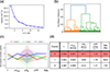 |
Fig. 4. Same as in Figure 3, but considering all three GSE components (total separation). |
| In the text | |
|
Fig. 5. Same as in Figure 3, but for Pc5 frequency range (2.5–10 min periods) in the GSE x-direction. |
| In the text | |
|
Fig. 6. Same as in Figure 3, but for fluctuations in the Pc5 frequency range (periods 2.5–10 min) and considering all three GSE components (total separation). |
| In the text | |
|
Fig. 7. Same as in Figure 3, but for fluctuations with periods between 10 and 30 minutes in the GSE-x direction. |
| In the text | |
|
Fig. 8. Same as in Figure 3, but for fluctuations with periods ranging from 10 to 30 minutes and considering all three GSE components (total separation). |
| In the text | |
Current usage metrics show cumulative count of Article Views (full-text article views including HTML views, PDF and ePub downloads, according to the available data) and Abstracts Views on Vision4Press platform.
Data correspond to usage on the plateform after 2015. The current usage metrics is available 48-96 hours after online publication and is updated daily on week days.
Initial download of the metrics may take a while.