| Issue |
A&A
Volume 705, January 2026
|
|
|---|---|---|
| Article Number | A217 | |
| Number of page(s) | 19 | |
| Section | Planets, planetary systems, and small bodies | |
| DOI | https://doi.org/10.1051/0004-6361/202557127 | |
| Published online | 29 January 2026 | |
Exomoon search with VLTI/GRAVITY around the substellar companion HD 206893 B
1
LIRA, Observatoire de Paris, Université PSL, Sorbonne Université, Université Paris Cité, CY Cergy Paris Université, CNRS,
92190
Meudon,
France
2
Center for Interdisciplinary Exploration and Research in Astrophysics (CIERA) and Department of Physics and Astronomy, Northwestern University,
Evanston,
IL
60208,
USA
3
European Southern Observatory,
Karl-Schwarzschild-Straße 2,
85748
Garching,
Germany
4
Department of Physics & Astronomy, Johns Hopkins University,
3400 N. Charles Street,
Baltimore,
MD
21218,
USA
5
Space Telescope Science Institute,
3700 San Martin Drive,
Baltimore,
MD
21218,
USA
6
Leiden Observatory, Leiden University,
Einsteinweg 55,
2333
CC
Leiden,
The Netherlands
7
Fakultät für Physik, Universität Duisburg-Essen,
Lotharstraße 1,
47057
Duisburg,
Germany
8
Center for Space and Habitability, Universität Bern,
Gesellschaftsstrasse 6,
3012
Bern,
Switzerland
9
Max Planck Institute for Astronomy,
Königstuhl 17,
69117
Heidelberg,
Germany
10
Universidade de Lisboa – Faculdade de Ciências, Campo Grande,
1749-016
Lisboa,
Portugal
11
CENTRA – Centro de Astrofísica e Gravitação, IST, Universidade de Lisboa,
1049-001
Lisboa,
Portugal
12
Univ. Grenoble Alpes, CNRS, IPAG,
38000
Grenoble,
France
13
Max Planck Institute for extraterrestrial Physics,
Giessenbachstraße 1,
85748
Garching,
Germany
14
Université Côte d’Azur, Observatoire de la Côte d’Azur, CNRS,
Laboratoire Lagrange, Bd de l’Observatoire, CS 34229,
06304
Nice cedex 4,
France
15
Aix Marseille Univ, CNRS, CNES, LAM,
Marseille,
France
16
STAR Institute, Université de Liège,
Allée du Six Août 19c,
4000
Liège,
Belgium
17
Department of Astrophysical & Planetary Sciences, JILA,
Duane Physics Bldg., 2000 Colorado Ave, University of Colorado,
Boulder,
CO
80309,
USA
18
1st Institute of Physics, University of Cologne,
Zülpicher Straße 77,
50937
Cologne,
Germany
19
Max Planck Institute for Radio Astronomy,
Auf dem Hügel 69,
53121
Bonn,
Germany
20
Universidade do Porto, Faculdade de Engenharia, Rua Dr. Roberto Frias,
4200-465
Porto,
Portugal
21
School of Physics, University College Dublin,
Belfield, Dublin 4,
Ireland
22
Astrophysics Group, Department of Physics & Astronomy, University of Exeter,
Stocker Road,
Exeter
EX4 4QL,
UK
23
Departments of Physics and Astronomy, Le Conte Hall, University of California,
Berkeley,
CA
94720,
USA
24
European Southern Observatory, Casilla
19001,
Santiago 19,
Chile
25
University of Exeter, Physics Building,
Stocker Road,
Exeter
EX4 4QL,
UK
26
Astronomy Department, University of Michigan,
Ann Arbor,
MI
48109,
USA
27
Academia Sinica, Institute of Astronomy and Astrophysics,
11F Astronomy-Mathematics Building, NTU/AS campus, No. 1, Section 4, Roosevelt Rd.,
Taipei
10617,
Taiwan
28
European Space Agency (ESA), ESA Office, Space Telescope Science Institute,
3700 San Martin Drive,
Baltimore,
MD
21218,
USA
29
Department of Earth & Planetary Sciences, Johns Hopkins University,
Baltimore,
MD,
USA
30
Max Planck Institute for Astrophysics,
Karl-Schwarzschild-Str. 1,
85741
Garching,
Germany
31
Excellence Cluster ORIGINS,
Boltzmannstraße 2,
85748
Garching bei München,
Germany
32
Institute of Astronomy, KU Leuven,
Celestijnenlaan 200D,
3001
Leuven,
Belgium
33
School of Physics & Astronomy, University of Southampton,
Southampton
SO17 1BJ,
UK
34
Universidad Nacional Autónoma de México. Instituto de Astronomía.
A.P. 70-264, 04510
Ciudad de México,
04510,
Mexico
35
Univ. Lyon, Univ. Lyon 1, ENS de Lyon, CNRS, Centre de Recherche Astrophysique de Lyon UMR5574,
69230
Saint Genis-Laval,
France
★ Corresponding author: This email address is being protected from spambots. You need JavaScript enabled to view it.
Received:
5
September
2025
Accepted:
20
November
2025
Abstract
Context. This study presents the first application of high-precision astrometry to search for exomoons around substellar companions, as this field remains largely unexplored.
Aims. We investigate whether the orbital motion of the companion HD 206893 B exhibits astrometric residuals consistent with the gravitational influence of an exomoon or binary planet.
Methods. Using the VLTI/GRAVITY instrument, we monitored the astrometric positions of HD 206893 B and c on short (days to months) and long (yearly) timescales. This enabled us to isolate potential residual wobbles in the motion of component B attributable to an orbiting moon.
Results. Our analysis reveals tentative astrometric residuals in the HD 206893 B orbit. If interpreted as an exomoon signature, these residuals correspond to a candidate (HD 206893 B I) with an orbital period of approximately 0.76 years and a mass of ~0.4 Jupiter masses. However, the origin of these residuals remains ambiguous and could be due to systematics. Complementing the astrometry, our analysis of GRAVITY R = 4000 spectroscopy for HD 206893 B confirms a clear detection of water, but no CO was found using cross-correlation. We also found that AF Lep b, and β Pic b are the best short-term candidates to look for moons with GRAVITY+.
Conclusions. Our observations demonstrate the transformative potential of high-precision astrometry in the search for exomoons and proves the feasibility of the technique to detect moons with masses lower than Jupiter and potentially down to less than Neptune in optimistic cases. Crucially, further high-precision astrometric observations with VLTI/GRAVITY are essential to verify the reality and nature of this signal and apply this technique to a range of planetary systems.
Key words: instrumentation: interferometers / techniques: interferometric / astrometry / planets and satellites: detection
© The Authors 2026
 Open Access article, published by EDP Sciences, under the terms of the Creative Commons Attribution License (https://creativecommons.org/licenses/by/4.0), which permits unrestricted use, distribution, and reproduction in any medium, provided the original work is properly cited.
This article is published in open access under the Subscribe to Open model. This email address is being protected from spambots. You need JavaScript enabled to view it. to support open access publication.
1 Introduction
The detection of satellites around extrasolar planets or substellar companions, termed exomoons, remains an elusive frontier in modern astronomy. Moreover, there is no definition of what an exomoon is, and some ambiguity remains as to whether it may include, for instance, binary planets. Some studies have suggested that objects orbiting planets could be distinguished based on the center of mass of the system (planet+object). If the center of mass is outside the planet then it would be classified as a binary planet rather than an exomoon (Stern & Levison 2002; Vanderburg & Rodriguez 2021). Exomoons transiting isolated planetary-mass objects have also been discussed in Limbach et al. (2021). Despite extensive observational efforts, no exomoon has been definitively confirmed to date. Numerous detection techniques have been actively pursued, though the intrinsic challenges of identifying such small, faint companions persist. The transit method represents the most prominent approach, leveraging distinctive light-curve signatures induced by planet-moon systems (Simon, Szatmáry, & Szabó 2007). Complementary constraints may be derived from transit timing variations (TTVs) and transit duration variations (TDVs; Sartoretti & Schneider 1999; Kipping 2009a,b). Large-scale transit surveys have already imposed stringent limits on exomoon occurrence rates, constraining Galilean-analogue systems to fewer than 0.38 moons per planet for planets orbiting between ~0.1 and 1.0 au (Kipping et al. 2015; Teachey et al. 2018).
Alternative detection methodologies face distinct limitations. Microlensing surveys have not demonstrated significant promise for exomoon detection due to inherent smearing out of the exomoon signal (Han & Han 2002). Radial velocity (RV) monitoring of planets themselves (rather than their host stars) has shown potential, yielding upper mass limits (e.g., m sin i = 2 MJup for < 5 day period moons around HR 8799 planets; Vanderburg & Rodriguez 2021). Recent advances combining high-contrast imaging with high-resolution spectroscopy now permit sensitivity to 1–4% mass-ratio companions at separations comparable to the Galilean moons (Ruffio et al. 2023). Nevertheless, detecting satellites with masses akin to those of Solar System moons (with a maximum satellite-to-planet mass ratio of around 10−4) remains beyond current capabilities.
To date, only a limited number of tentative exomoon candidates have emerged. The Jupiter-sized transiting planet Kepler-1625 b has drawn particular attention due to light-curve anomalies suggestive of a Neptune-mass satellite (Teachey & Kipping 2018). However, the interpretation remains contested, with studies attributing the signal to an artifact of the data reduction, stellar activity, or unknown systematics (Heller, Rodenbeck, & Bruno 2019; Kreidberg, Luger, & Bedell 2019). Similarly debated is the proposed Neptune-sized companion to the super-Jupiter Kepler-1708 b (Kipping et al. 2022; Heller & Hippke 2024). Other candidates include a wider-separation Jupiter-mass companion to the brown dwarf DH Tau B (projected separation: 10 au; mass ratio 0.1; Lazzoni et al. 2020) and a 1.7 R⊕ object orbiting a free-floating planet (Limbach et al. 2021).
The scarcity of detections contrasts sharply with the ubiquity of moons in our Solar System (>300 confirmed), underscoring the observational challenges posed by sub-Earth-sized exomoons. Intriguingly, proposed candidates exhibit masses vastly exceeding those of solar system satellites (with typical mass ratios ~10−4 for Galilean moons), suggesting initial discoveries may occupy the extreme end of the exomoon mass spectrum. This parallels early exoplanet surveys, which revealed unexpected populations such as hot Jupiters. Theoretical works now support the plausibility of massive exomoons, either via gravitational capture (Hansen 2019) or formation within massive circumplanetary disks (Moraes & Vieira Neto 2020). Notably, moon masses could scale with the host planet mass as ![Mathematical equation: $\[\mathrm{M}_{p}^{3 / 2}\]$](/articles/aa/full_html/2026/01/aa57127-25/aa57127-25-eq1.png) (Batygin & Morbidelli 2020), favoring searches around super-Jovian planets or brown dwarfs, as in this study.
(Batygin & Morbidelli 2020), favoring searches around super-Jovian planets or brown dwarfs, as in this study.
Stability considerations further refine detection strategies. Exomoons must reside between their host’s Roche limit and ~0.49 RHill (prograde orbits) or 0.93 RHill (retrograde orbits; Domingos, Winter, & Yokoyama 2006). Close-in planets (<1 au) are poor candidates due to tidal destabilization (Dobos et al. 2021), necessitating focus on wider-orbit systems. This motivates the application of high-precision astrometry, capable of probing distant planets.
In this work, we demonstrate the potential of the VLTI/GRAVITY instrument to detect exomoons via astrometric monitoring. GRAVITY’s tens of microarcsecond-level precision enables direct tracking of planetary orbital wobbles induced by massive satellites, probing periods spanning days to years – a regime where stable, detectable exomoons are most likely to reside.
We present observations of the brown dwarf HD 206893 B (mass ~23 MJup, semimajor axis ~9 au, age ~110 Myr; Sappey et al. 2025, but see our new fit that leads to a lower mass and larger semimajor axis), a benchmark target for probing substellar companions. First identified with SPHERE (Milli et al. 2017) around the F5V star HD 206893 (distance: ~40.8 pc, Gaia Collaboration 2020), its properties remain a matter of debate: comparing the atmosphere properties from atmospheric models with evolutonary tracks suggest a possible younger age down to 3 Myr, and a planetary-mass regime as low as 5 MJup (Kammerer et al. 2021). Notably, HD 206893 B exhibits spectral characteristics of an L/T transition object, with extreme near-infrared colors indicative of high-altitude dust clouds (Delorme et al. 2017; Ward-Duong et al. 2021; Kammerer et al. 2021).
The HD 206893 system hosts a complex architecture (see Fig. 1). A ~10 MJup planetary-mass companion, HD 206893 c, orbits interior to the brown dwarf at ~3.6 au (Hinkley et al. 2023; Sappey et al. 2025). ALMA observations further reveal a structured debris disk extending from 30 to 180 au, bisected by a 27 au gap (Marino et al. 2020). This gap may harbor an additional Jupiter-mass companion at ~75 au, which, if confirmed, would constitute a third companion in the system.
Our analysis focuses on two key aspects: (1) quantifying GRAVITY’s sensitivity to exomoon-induced astrometric perturbations through precision monitoring of HD 206893 B’s orbital motion and (2) conducting the first medium-resolution (R = 4000) K-band spectral analysis of HD 206893 B’s atmosphere using GRAVITY data. By modeling the brown dwarf’s astrometric residuals, we established detection limits for potential satellites and assessed the instrument’s capability to resolve exomoon dynamical signatures. Moreover, we refined the orbits of HD 206893 B and c, using our new data. Simultaneously, the spectroscopic data can provide new insights into the atmospheric composition and cloud properties of this enigmatic L/T transition object.
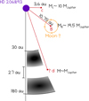 |
Fig. 1 Schematic of the HD 206893 system. |
GRAVITY astrometry for HD 206893, along with its B and c components.
2 Observations and data reduction
HD 206893 B was observed with the GRAVITY instrument (GRAVITY Collaboration 2017) at the VLTI during eight epochs between April and July 2024 (Prog. ID 113.26D9.001). These observations complement those obtained as part of the Exo-GRAVITY large program (Lacour et al. 2020). A final observation was conducted in June 2025 as part of the commissioning of the new adaptive optics system of GRAVITY+. An observing log for all epochs is provided in Table D.1. During the 2024 observing campaign, a short observational cadence was adopted to maximize sensitivity to moon-like companions around HD 206893 B. This strategy enhances the sensitivity to moons orbiting the brown dwarf companion on timescales of days to months.
All data were obtained with the four 8.2 m Unit Telescopes (UTs) in dual-field on-axis mode. In this configuration, a 50/50 beamsplitter directed half of the starlight to the GRAVITY fringe tracker, while the other half (either from the star or the companion) was sent to the GRAVITY science spectrometer, which was operated at a spectral resolving power of R ~ 4000 in the K-band (~2–2.4 μm). This setup allowed for the calibration of the companion exposures using the host star exposures, eliminating the need for dedicated calibrator observations.
The data were reduced using the ESO GRAVITY pipeline version 1.6.4b and further processed with the GRAVITY Consortium Python tools1 to extract relative astrometry and K-band contrast spectra (relative to the host star) of HD 206893 B (Lapeyrere et al. 2014). The data reduction followed the procedure described in Appendix A of GRAVITY Collaboration (2020). A recent improvement was achieved by down-weighting baselines that have a high degree of self-subtraction caused by post-processing. This allowed for a more aggressive suppression of the stellar flux by increasing the order of the polynomial fit, without excessively amplifying systematic noise. Reductions were therefore performed using different polynomial orders for the post-processing (see the impact of polynomial order in Lacour et al. 2025), specifically orders 3, 4, and 6. The resulting astrometry is listed in Table D.2. All the datasets were uniformly reduced to result in the astrometry adopted in this paper, summarized in Table 1.
To convert the contrast spectra into flux-calibrated spectra, we multiplied them by a model spectrum of the host star HD 206893 A. For this purpose, we fit a BT-NextGen stellar atmosphere model (Allard et al. 2012) to archival photometry from Gaia, 2MASS, Tycho, and WISE, as well as the Gaia XP-spectrum (Carrasco et al. 2021; De Angeli et al. 2023) of HD 206893 A. Interstellar extinction was not included in the fit, as the Gaia DR3 catalog reports a G-band extinction of 0 mag (Gaia Collaboration et al. 2023). The surface gravity was fixed to the Gaia DR3 value of log g = 4.13. The fit yields an effective temperature of ![Mathematical equation: $\[6554_{-27}^{+29}\]$](/articles/aa/full_html/2026/01/aa57127-25/aa57127-25-eq2.png) K, consistent within 1σ with the value reported by Delorme et al. (2017). Figure 2 displays the resulting model spectrum for HD 206893 A, along with the archival photometry used in the fit, providing a good fit in band K.
K, consistent within 1σ with the value reported by Delorme et al. (2017). Figure 2 displays the resulting model spectrum for HD 206893 A, along with the archival photometry used in the fit, providing a good fit in band K.
The companion flux spectra were then obtained by multi-plying the GRAVITY contrast spectrum with the stellar model spectrum. We propagated the uncertainties of the stellar model and the correlations of the GRAVITY spectra throughout the entire process. This yielded a companion flux spectrum for each epoch. To obtain the highest possible signal-to-noise ratio (S/N), the individual epochs are then averaged together to a final companion flux spectrum by computing a covariance-weighted mean spectrum. Before, though, we applied scaling factors to each individual epoch to bring them into better agreement with each other. The best fitting scaling factors are shown in Fig. A.1. The scaling factors were introduced to mitigate the ~10% systematic flux variability between epochs caused by variations in the PSF shape due to atmospheric turbulence and instrumental effects. The final companion flux average spectrum is shown in Fig. 3.
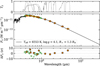 |
Fig. 2 Model spectrum of HD 206893 A obtained by fitting a BT-NextGen stellar model atmosphere (black line) to archival photometry (orange points) and the Gaia XP spectrum (green points). The top panel shows the filter transmission curves and the bottom panel shows the residuals between the data and model. |
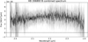 |
Fig. 3 Combined R ~ 4000 spectrum obtained with GRAVITY for HD 206893 B by averaging the data obtained at different epochs (see Fig. A.1). |
3 Exomoon search and new predictions for the orbits of HD 206893 B and c
3.1 Back of the envelope predictions for the moon’s astrometric effect
We considered a moon with a mass represented by Mmoon orbiting a planet of mass, Mpla. They were both assumed to orbit around their barycenter, with the semimajor axis of the planet’s orbit due to the exomoon given by
![Mathematical equation: $\[a_{\mathrm{ast}}=a_{\mathrm{moon}} \frac{M_{\mathrm{moon}}}{M_{\mathrm{pla}}+M_{\mathrm{moon}}} \approx q ~a_{\mathrm{moon}},\]$](/articles/aa/full_html/2026/01/aa57127-25/aa57127-25-eq3.png) (1)
(1)
where amoon is the distance between the planet and the moon, and q is the moon-to-planet mass ratio Mmoon/Mpla.
If we define the maximum astrometric angular displacement Δ for a full orbit of the planet around its barycenter due to the moon’s gravity, we get
![Mathematical equation: $\[\Delta=\frac{2 a_{\mathrm{ast}}}{d},\]$](/articles/aa/full_html/2026/01/aa57127-25/aa57127-25-eq4.png) (2)
(2)
where d is the system’s distance to the Sun (see Fig. 4). Then, we can readily derive
![Mathematical equation: $\[q=\left[\frac{2 a_{\mathrm{moon}}}{d \Delta}-1\right]^{-1}.\]$](/articles/aa/full_html/2026/01/aa57127-25/aa57127-25-eq5.png) (3)
(3)
We note that this derivation assumes that we measure the wobble of the giant planet or companion, while we can actually measure the wobble of the center of light of the pair with GRAVITY (Kral et al. 2016). The moon may have a non-negligible flux contribution depending on its albedo in the infrared compared to the host. However, it is neglected in this study, given uncertainties, and that we consider moons with much lower masses than the moon host.
If the orbit has an eccentricity, e, then the minimum astrometric displacement seen on the sky would be twice the semiminor axis, ![Mathematical equation: $\[b_{\text {ast}}=a_{\text {ast}} \sqrt{1-e^{2}}\]$](/articles/aa/full_html/2026/01/aa57127-25/aa57127-25-eq6.png) , so that
, so that ![Mathematical equation: $\[\Delta=2 a_{\text {ast }} \sqrt{1-e^{2}} / d\]$](/articles/aa/full_html/2026/01/aa57127-25/aa57127-25-eq7.png) . In this case, we obtained (Ruffio et al. 2023):
. In this case, we obtained (Ruffio et al. 2023):
![Mathematical equation: $\[q=\left[\frac{2 a_{\mathrm{moon}} \sqrt{1-e^2}}{d \Delta}-1\right]^{-1}.\]$](/articles/aa/full_html/2026/01/aa57127-25/aa57127-25-eq8.png) (4)
(4)
For simplicity, assuming that the eccentricity is zero and that q ≪ 1, then we obtain
![Mathematical equation: $\[q=\frac{1}{2}\left(\frac{a_{\mathrm{moon}}}{\mathrm{au}}\right)^{-1}\left(\frac{d}{\mathrm{pc}}\right)\left(\frac{\Delta}{1^{\prime \prime}}\right),\]$](/articles/aa/full_html/2026/01/aa57127-25/aa57127-25-eq9.png) (5)
(5)
or converting to the period Tmoon of the orbit using Kepler’s third law, we finally obtain
![Mathematical equation: $\[\frac{M_{\mathrm{moon}}}{\mathrm{M}_{\mathrm{Nep}}}=0.48\left(\frac{T_{\mathrm{moon}}}{10 \mathrm{~d}}\right)^{-2 / 3}\left(\frac{d}{10 ~\mathrm{pc}}\right)\left(\frac{\Delta}{10 ~\mu \mathrm{as}}\right)\left(\frac{M_{\mathrm{pla}}}{10 ~\mathrm{M}_{\mathrm{Jup}}}\right)^{2 / 3},\]$](/articles/aa/full_html/2026/01/aa57127-25/aa57127-25-eq10.png) (6)
(6)
where MNep is Neptune’s mass equal to 17.15 M⊕, and MJup the Jupiter’s mass equal to 317.8 M⊕. In the formula above, we use units of day, parsec, and microarcsec for the period, distance, and astrometric signature, respectively. This equation shows that exomoons with masses around that of Neptune may be targeted with an astrometry at 10 μas level for the closest systems. It may even go down to an Earth mass for moons located at larger periods and down to the mass of the Jupiter moon Ganymede of mass MGanymede ~ 0.025 M⊕ around less massive planets than assumed here (10 MJup) located at larger distances from the central star with their Hill spheres being much larger, allowing for stable moons at several year periods. To better visualize this equation, we plot it in Fig. 5.
As stated earlier, the moon should remain within the planet’s Hill sphere RHill = apla (1 − epla)(Mpla/(3M⋆))1/3, where apla is the planet’s semimajor axis, epla the planet’s eccentricity, and M⋆ the stellar mass. The moon should also be located beyond the Roche limit (Roche 1849) defined as Rroche = Rpla (4πρpla/(γρmoon))1/3, where Rpla is the planet’s radius, ρpla the planet’s density, ρmoon the moon’s density, and γ is a dimensionless geometrical parameter with γ = 4π/3 for a sphere, but is smaller for an object that takes a non-spherical shape (Murray & Dermott 1999). Porco et al. (2007) find that γ = 1.6 may be more realistic for moon-lets. In the case of an incompressible fluid, taking full account of the feedback between the moon’s deformed shape and its gravity field smoothes the cusps and elongates the moon further (Chandrasekhar 1969; Murray & Dermott 1999), leading to an even smaller value, γ ≈ 0.85. This sets some limits on the moon’s period, such that, within the Hill sphere, we have
![Mathematical equation: $\[\frac{T_{\mathrm{moon}}}{\mathrm{yr}}<18\left(\frac{M_{\star}}{\mathrm{M}_{\odot}}\right)^{-1 / 2}\left(\frac{a_{\mathrm{pla}}}{10 ~\mathrm{au}}\right)^{3 / 2}\left(1-e_{\mathrm{pla}}\right)^{3 / 2},\]$](/articles/aa/full_html/2026/01/aa57127-25/aa57127-25-eq11.png) (7)
(7)
and beyond the Roche limit, we have
![Mathematical equation: $\[\frac{T_{\text {moon }}}{\mathrm{d}}>0.5\left(\frac{\gamma}{1}\right)^{-1 / 2}\left(\frac{\rho_{\text {moon }}}{1000 \mathrm{~kg} / \mathrm{m}^3}\right)^{-1 / 2},\]$](/articles/aa/full_html/2026/01/aa57127-25/aa57127-25-eq12.png) (8)
(8)
leading to typical moon periods between a day and several decades, but we note the strong dependence on the planet semimajor axis apla, which can push the Hill radius to 210-day period for apla = 1 au instead of 18 yr for 10 au, or 580 yr for 100 au.
Next, we focused on the HD 206893 system and produced a prediction for the presence of an exomoon around HD 206893 B using its specific set of parameters. Using that d = 40.8 pc, Mpla = 19.5 MJup (see the next section), we plotted the moon mass model prediction as a function of moon period in Fig. 6. We also adapted the Hill radius by using M⋆ = 1.31 M⊙, apla = 10.75 au, and epla = 0.07 (see our fit in the next section). In addition, we show a green point obtained by fitting the GRAVITY data that represents upper limits in moon mass and period derived in Sect. 3.3 (i.e. an upper limit of 0.8 MJup in mass and using the tentative detection semimajor axis of 0.22 au or 278 days). The orange area represents the allowed parameter space of a plausible moon that would hide around HD 206893 B, but would still be detectable with GRAVITY given an astrometric accuracy of 10 μas. We note that the orange zone extends slightly beyond the analytical predictions because our upper limit accounts for different orientations of the system (e.g., obliquity, inclination), whereas the analytical model does not.
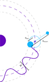 |
Fig. 4 Diagram of the orbit of HD 206893 B with a potential moon around it, causing it to shift slightly due to the moon’s gravitational potential. It illustrates the notation used in Sect. 3.1. |
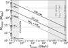 |
Fig. 5 Analytical predictions of Mmoon (the mass of the moon in masses of Neptune) as a function of Tmoon (the period of the moon in days). The solid black lines show the model’s prediction for astrometric accuracies of 10 and 100 μas, as indicated on the graph. The values used are those of Eq. (6), i.e., d = 10 pc and Mpla = 10 MJup. The dotted line shows the case of 10 μas considering Mpla = 1 MJup. If the system is instead at 100 pc, the lines are pushed up by a factor of 10. The areas beyond the Roche limit and the Hill sphere are shown in grey. The Hill sphere is shown for two values of the semimajor axis of the planet apla equal to 1 (closest) and 10 au (farthest). The horizontal lines indicate moon masses of 1 MJup, 1 MNep, 1 M⊕, and 1 MGanymede from top to bottom. |
3.2 Refining the orbit of HD 206893 B and c
We repeated the orbit modeling following the procedure described in Hinkley et al. (2023) to obtain updated orbital posteriors for HD 206893 B and c. We fit the relative astrometry, Hipparcos-Gaia absolute astrometry from the EDR3 edition of the HGCA (Brandt 2021), and stellar radial velocity data (Grandjean et al. 2019; Hinkley et al. 2023) using orbitize! (Blunt et al. 2020, 2024). We did not include the companion radial velocity of B measured in Sappey et al. (2025), as it did not provide any additional constraints to the orbit fit.
We used the parallel-tempered affine-invariant sampler ptemcee (Foreman-Mackey et al. 2013; Vousden et al. 2016) with 20 temperatures and 1000 walkers per temperature to sample the posterior. We discarded the first 35 000 steps as “burn-in” after visual inspection of the walkers, using only the last 5000 steps from the lowest temperature walkers to construct the posterior. We present the updated orbital parameters in Table 2.
In broad strokes, the orbital configuration of the two planets remains the same as that reported in Hinkley et al. (2023). The substantial increase in GRAVITY astrometry of B has resulted in a much more precise orbit solution for both planets, since the visual orbit of B also contains information on the orbit of c (similar to GRAVITY observations of β Pic b and c; Lacour et al. 2021). The orbit of HD 206893 B is nearly circular, and with a 1 au larger semimajor axis than what was found in Hinkley et al. (2023). This results in a dynamical mass for B that is 8 MJup lower than what was found in Hinkley et al. (2023). The orbit of HD 206893 c is also more circular (![Mathematical equation: $\[0.283_{-0.017}^{+0.019}\]$](/articles/aa/full_html/2026/01/aa57127-25/aa57127-25-eq13.png) compared to
compared to ![Mathematical equation: $\[0.41_{-0.03}^{+0.03}\]$](/articles/aa/full_html/2026/01/aa57127-25/aa57127-25-eq14.png) ) and is now nearly coplanar with HD 206893 B. This is a much more dynamically stable configuration than the nearly unstable orbital solution found in Hinkley et al. (2023). The epicyclic motion in the visual orbit of B due to the orbit of c can now be detected in the GRAVITY data, which helps constrain the orbit of c, in contrast to the previous process that relied heavily on the stellar RV and astrometry.
) and is now nearly coplanar with HD 206893 B. This is a much more dynamically stable configuration than the nearly unstable orbital solution found in Hinkley et al. (2023). The epicyclic motion in the visual orbit of B due to the orbit of c can now be detected in the GRAVITY data, which helps constrain the orbit of c, in contrast to the previous process that relied heavily on the stellar RV and astrometry.
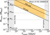 |
Fig. 6 Analytical predictions for the astrometric effect of a moon with varying mass and distance to HD 206893 B. GRAVITY could in principle detect moons lower than a Neptune mass at larger periods. The fit of the GRAVITY data is shown as a green point assuming the mass and period as upper limits in our tentative detection. The orange area shows the plausible parameter space where a moon might be located, and still be potentially detectable with GRAVITY assuming an astrometric accuracy of 10 μas (see Sect. 3.3). |
3.3 Fit of astrometric residuals to look for an exomoon
To search for a possible companion orbiting HD 206893 B, we performed a three-body hierarchical fit with orbitize!. In this hierarchical model, we assume a companion is orbiting B and that the barycenter of these two bodies orbits around the star. This is implemented in practice in orbitize! by setting B to be body 0, the potential companion to B to be body 1, and the host star HD 206893 to be body 2, and by setting a non-zero mass for B (19.5 MJup; Table 2). In addition to the gravitational influence of the host star and any potential moon, the orbit of B is also influenced by c. This is not captured by the hierarchical model implemented in orbitize!. Thus, we subtract out the perturbations in the visual orbit of B due to the gravitational influence of c (i.e., c causing the star to move about the system barycenter, which is encoded in the relative astrometry between B and the host star; see Lacour et al. 2021), using the maximum posterior probability orbit from the previous section.
For simplicity, we assumed the potential orbital companion to HD 206893 B is on a circular orbit. We also set priors on the mass of the potential companion to be between 10−3 and 10 MJup and the semimajor axis to be between 0.001 and 1 AU. We did not place any constraints on the orbital orientation of the moon relative to the orbit of B. We used ptemcee to sample the orbital posterior using 20 temperatures and 1000 walkers per temperature. We discarded the first 10 000 steps of each walker as burn-in after visual inspection, and used the remaining 10 000 steps of each lowest-temperature walker to construct the posterior.
The posterior for the potential exomoon’s semimajor axis (SMA), inclination (INC), position angle of ascending nodes (PAN), and mass are shown in Fig. 7. Assuming no moon detection, we have a 95% upper limit on the mass of the moon at 0.8 MJup. However, we do find a peak in the moon SMA 1-D marginalized posteriors at about 0.22 au (period of 0.76 yr). The inclination (INC) and position angle of the ascending node (PAN) are moderately constrained, with the best-fit values around 90 deg, which would be ~60 degrees misaligned from the orbit of B.
To analyze the most promising peak in the posterior, we considered only the posterior samples between 0.21 and 0.26 au. The posterior is plotted in Fig. B.1. In this case, the moon mass seems to converge to a value around 0.5 MJup. We phase-folded the data based on this orbital period (0.76 yr) and compared it to the orbital model. The phase-folded residual plot shows the potential RA and Dec offsets on HD 206893 B after accounting for the planet c influence and removing the HD 206893 B orbit motion (Fig. 8). The offsets from 0 in the residuals are due to uncertainty in the orbit of HD 206893 B itself, while the sinusoidal wiggles are mainly caused by the moon in our orbital model. We also visualized the residuals on a RA vs. Dec plot in Fig. 9 (we also removed the average motion due to HD 206893 B orbiting the star and accounting for the motion induced by the planet c), where we see that the data seems to form an ellipse around the origin. The data seem to be well traced by exomoon trajectories from our model that are ~0.15 mas in radius. We note that for a moon of mass 0.5 MJup orbiting at 0.22 au from B of mass 19.5 MJup, then it causes the B component to orbit around a center of gravity that is located at about 0.5 ÷ 19.5 × 0.22 = 0.0056 au or ~0.14 mas, which is indeed similar to what we observe on the RA Vs Dec plot. However, we note that systematic errors in the astrometry can also cause the data to form an ellipse around the origin.
Systematic errors can have multiple origins. Table 1 in Lacour et al. (2014) provides a review of their possible sources, including improper baseline calibration, terrestrial reference frame uncertainties, atmospheric dispersion, optical aberrations, and others. All of these effects were carefully evaluated and constrained to remain below 10 μas. Laser trackers were used for baseline calibration; updates of the Earth orientation parameters (EOP) and the difference between astronomical time (UT1) and coordinated universal time (UTC) are regularly obtained from the International Earth Rotation and Reference Systems Service (IERS); and optical aberrations within our system were measured and their impact assessed (GRAVITY Collaboration et al. 2021). Overall, we are confident that these known systematics do not dominate the error budget.
To test the hypothesis that the tentative detection might be real, we ran a simulation with no moons and compared it with the results of our previous fit, including a moon, by using the Bayesian information criterion (BIC). The median BIC favours the exomoon fit over the no moon fit by 7.4, which could point to some real signal but is less than the threshold of 10 that would be needed to decisively favor the exomoon model (Liddle 2007). In particular, the exomoon model could be used to fit for unaccounted systematics in our data. Therefore, our data do not allow us to confirm the presence of an exomoon for now and further observations are needed. Furthermore, the BIC test does not take into account any systematic errors in the astrometry, which the exomoon model could be fitting for.
We conclude that we find an upper limit of a potential moon around HD 206893 B of 0.8 MJup, using the 95th percentile limit or 0.5 MJup (or 9.3 MNep), if we assume a tentative detection. We also see that the SMA is peaking at a value around 0.22 au, but we note that there are other smaller peaks around and we cannot be certain that the period around 0.76 yr is real. More data from GRAVITY on a monthly timescale would allow us to draw a more firm conclusion.
Orbital fit of the B and c components in the HD 206893 system.
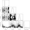 |
Fig. 7 Fit of the astrometric data of HD 206893 B looking for an exomoon. The MCMC analysis finds a 95% upper limit of 0.8 MJup for the potential exomoon mass and a peak in semimajor axis at 0.22 au, while the inclination and position angle of ascending node are around 90 deg. Another MCMC plot assuming a fixed semimajor axis around its peak is shown in Fig. B.1. |
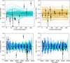 |
Fig. 8 Residuals of HD 206893 B orbit after removing the average motion due to HD 206893 B orbiting the star and accounting for the motion induced by the planet c. In the top two plots, the data are phase-folded by a period of 275 days, using MJD 58500 as the starting point. 50 random draws with SMA between 0.21 and 0.26 AU are plotted in cyan for the RA and orange for the Dec Vs time plots, respectively. These model draws have the average motion of HD 206893 B removed, so they show both perturbation from the exomoon model and the residuals in the orbit of B from the average orbit of B. In the bottom plots, the data are plotted as a function of MJD and not phase-folded. The orbits are colored by orbital phase, where blue is an orbital phase of 0 and green is an orbital phase of 1. Note: the orbital periods vary between each model drawn and are slightly different from an exact 275-day orbital period. |
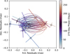 |
Fig. 9 Similar residuals as Fig. 8, but projected onto the 2-D sky plane and the 50 random draws from the posterior only consider the motion of a potential exomoon (and not residual uncertainties in the orbit of B, which are shown in Fig. 8). The colors of both the data and the models correspond to the 275-day phase, as specified by the colorbar and defined in Fig. 8. |
4 Spectral analysis
Together with the astrometric observation of HD 206893 B, we obtained an R = 4000 spectrum of the object. A previous spectrum at R = 500 was previously published in Kammerer et al. (2021) and in Sappey et al. (2025) at a higher resolution (R = 35 000). Moreover, SPHERE observations led to the detection of water at 1.4 microns (Delorme et al. 2017).
4.1 Atmospheric forward modeling
We performed forward model fitting of the GRAVITY spectrum using the Bayesian framework Species (Stolker 2023), and several pre-computed atmospheric grids designed for young giant planets at medium spectral resolution: Exo-REM (Charnay et al. 2018; Blain et al. 2021), ATMO (grid from Petrus et al. 2025) and, for comparison, the commonly used BT-Settl grid (Allard & Homeier 2012). These models are designed for late-M to earlyT type objects and differ mainly in their treatment of clouds and thermal structure. BT-Settl includes microphysical processes and settling to account for clouds; while Exo-REM adds simple cloud microphysics and disequilibrium chemistry relevant for late L and early T dwarfs; ATMO is cloud-free model but incorporates diabatic processes that modify the temperature gradient via an effective adiabatic index γ. For computational efficiency, we limited the fit to an effective temperature range of 1000–1900 K. Results are in Figs. C.1, C.2, and C.3 for each model. Figure C.4 displays the best fit spectra together with the GRAVITY data). The BT-Settl models yield higher effective temperatures and smaller radii, with Teff = ![Mathematical equation: $\[1582_{-29}^{+16}\]$](/articles/aa/full_html/2026/01/aa57127-25/aa57127-25-eq34.png) K and R = 0.93 RJup, likely due to the cloud modeling prescription. In contrast, Exo-REM and ATMO provide broadly consistent effective temperatures, Teff =
K and R = 0.93 RJup, likely due to the cloud modeling prescription. In contrast, Exo-REM and ATMO provide broadly consistent effective temperatures, Teff = ![Mathematical equation: $\[1162_{-67}^{+158}\]$](/articles/aa/full_html/2026/01/aa57127-25/aa57127-25-eq35.png) K and Teff =
K and Teff = ![Mathematical equation: $\[1097_{-50}^{+60}\]$](/articles/aa/full_html/2026/01/aa57127-25/aa57127-25-eq36.png) K, respectively, and larger radii (Rp =
K, respectively, and larger radii (Rp = ![Mathematical equation: $\[1.79_{-0.35}^{+0.24}\]$](/articles/aa/full_html/2026/01/aa57127-25/aa57127-25-eq37.png) RJup) for Exo-REM and R =
RJup) for Exo-REM and R = ![Mathematical equation: $\[1.98_{-0.30}^{+0.28}\]$](/articles/aa/full_html/2026/01/aa57127-25/aa57127-25-eq38.png) RJup for ATMO. Models yield to the following C/O values,
RJup for ATMO. Models yield to the following C/O values, ![Mathematical equation: $\[0.38_{-0.20}^{+0.20}\]$](/articles/aa/full_html/2026/01/aa57127-25/aa57127-25-eq39.png) for Exo-REM, and
for Exo-REM, and ![Mathematical equation: $\[0.37_{-0.05}^{+0.09}\]$](/articles/aa/full_html/2026/01/aa57127-25/aa57127-25-eq40.png) for ATMO, consistent with subsolar C/O ratios up to solar abundances for Exo-REM given the uncertainties.
for ATMO, consistent with subsolar C/O ratios up to solar abundances for Exo-REM given the uncertainties.
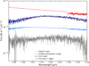 |
Fig. 10 Comparison between the GRAVITY combined spectrum (gray) and the ExoREM synthetic spectrum for T = 1400 K (light blue). Each species spectrum is shown with an offset with different colours – dark blue for water, pink for sodium, and red for CO. |
4.2 Cross-correlation
Cross-correlations between model spectra and observed data is a commonly used technique to detect molecular species in the atmospheres of directly imaged exoplanets and brown dwarfs (e.g., Konopacky et al. 2013; de Regt et al. 2024). We cross-correlated the GRAVITY spectrum obtained in Fig. 3 with synthetic spectra generated using the ExoREM atmospheric model (Charnay et al. 2018; Blain et al. 2021), assuming a range of effective temperature, log(g) = 4.0, solar metallicity, and a C/O ratio of 0.5. We found that an effective temperature of 1400 K provided the highest S/N, although the measured S/N remain similar across effective temperatures from 1100 to 1400 K. We focused on the main species expected to contribute in the K band spectral range (i.e., H2O, CO), as predicted by the ExoREM model (see Fig. 10). Although NH3 and H2S also exhibit spectral features, they are too faint to be detected in our data.
The observed spectrum was first smoothed using a Gaussian filter with σ = 10 pixels. This smoothed spectrum is then subtracted to focus solely on the high-frequency components of the observed spectrum. The wavelength grid is sampled logarithmically, corresponding to a radial-velocity spacing of Δv = 5 km s−1, and both the model and observed spectra are interpolated onto this new grid. The CCF was then computed using the scipy.signal.correlate routine and normalized by the square root of the sum of the model and the data spectrum squared. We note that we did not include any broadening of the model given the low spectral resolution of the data.
To account for the intrinsic autocorrelation of the model spectrum (which can be particularly strong for molecules with strong harmonic features such as CO), we also computed the autocorrelation function (ACF) of each model. This correction was performed by subtracting a rescaled ACF from the CCF wings (±200 km/s). Figure 11 displays each CCF along with the S/N of its peak.
The S/N was computed as the peak divided by the standard deviation of the CCF wings (between 500 km/s and 3000 km/s); we display the S/N with and without the autocorrelation corrected in the figure’s legend. Restricting the analysis to the 2.2–2.4 μm range, where water, CO features dominate, further improved the S/N of the detections. The full-model CCF yields a peak S/N of 5.3, with the H2O-only template yielding an S/N of 4.16. While no significant signal was detected for CO, the absorption band at 2.3 μm appears to be visible in the spectrum (Fig. 10). The CCF peaks of H2O and of the full model appeared around −35 km/s, though this offset remains below the instrumental resolution of GRAVITY of about 75 km/s. We note that the star radial velocity is −12.45 km/s (Gaia Collaboration 2018), which is in the appropriate range.
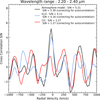 |
Fig. 11 Cross-correlation S/N peaks between the data and the ExoREM synthetic spectrum for T = 1400 K. The global cross-correlation S/N are computed as the peak divided by the standard deviation of the CCF wings (500 to 3000 km/s), with their final values displayed in the legend for each species (in colour) and for the global atmospheric model (in black). |
5 Discussion
5.1 Target selection for GRAVITY+
Based on their respective distances, host star separations, and magnitudes, we filtered the Encyclopaedia of exoplanetary systems (exoplanet.eu, Schneider et al. 2011) for planets that would prove viable for a follow-up with GRAVITY+ aimed at detecting exomoons. First, we selected confirmed planets and brown dwarfs exhibiting masses between 1 and 30 MJup. Lower-mass objects would not be bright enough to be detectable with GRAVITY+. We also decided to remove free-floating planets because they are not yet accessible to GRAVITY+ without laser guide stars, as a bright reference source nearby is needed. Next, we only retained the planets with semimajor axes greater than 1 au and smaller than 100 au because they would need to be adequately separated from the star to be detectable with GRAVITY+. The eccentricities were set lower than 0.3 to avoid overly complex dynamics in the potential moon systems. We also removed all planets detected around pulsars or other exotic objects. Finally, we selected only systems closer than 1000 pc from Earth, as astrometric signals from exomoons would become too small for overly distant systems.
We show the resulting objects after this initial selection in Fig. 12, representing the planetary mass, Mpla, as a function of the target system distance, d. The respective semimajor axis apla is shown in colour. At this stage, the sample consists of 124 planets. We circled in red the 14 objects that have already been observed with GRAVITY. Next, we selected the best 25 targets, namely, those with the smallest d values that have an angular distance greater than 0.08 arcsec (i.e., detectable with GRAVITY).
Using the ATMO (Phillips et al. 2020), AMES-Dusty (Chabrier et al. 2000; Allard et al. 2001), and AMES-Cond (Allard et al. 2001; Baraffe et al. 2003) evolutionary models, we computed the K-band magnitude expected for these most favourable targets. To this end, we used the available planet masses and system ages listed in exoplanet.eu, discarding targets for which these estimates were missing. The resulting magnitudes are listed in Table 3. Since the different evolutionary models were designed to handle a diverse set of objects, the resulting magnitude estimates are model-dependent. For instance, while the ATMO model lacks a cloud prescription, AMES-Dusty is capable of describing cloudy atmospheres. No estimates were possible for objects with mass or age estimates outside the ranges in which the models are defined. Some models could not be run when the evolutionary models were not defined in mass or age, leading to a few empty values seen in Table 3.
In general, a GRAVITY+ follow-up requires a companion brighter than K = 20 mag. This narrows down the follow-up sample to five viable targets, namely, 2MASS J1315-2649 b (full name: 2MASS J13153094-2649513 b; Burgasser et al. 2011), β Pic b (Lagrange et al. 2010), AF Lep b (Franson et al. 2023), HD 155555 (AB) b (Asensio-Torres et al. 2018; Gratton et al. 2023), and HD 60584 b, where the latter needs to be confirmed (Bonavita et al. 2022). Two of these, β Pic b (GRAVITY Collaboration 2020) and AF Lep b (Balmer et al. 2025), were already observed with GRAVITY. Finally, we retrieved the K-band fluxes of the individual hosts from the 2MASS All-Sky Catalogue (Cutri et al. 2003) and ensured that the host-to-companion contrast is within 105 to be able to detect them with GRAVITY. All targets pass the contrast test, and this does not affect our previous list.
According to Eq. (6), the moon mass detectable with GRAVITY scales as ![Mathematical equation: $\[T_{\text {moon }}^{-2 / 3}\]$](/articles/aa/full_html/2026/01/aa57127-25/aa57127-25-eq41.png) (moon’s period), d (distance to Earth), and
(moon’s period), d (distance to Earth), and ![Mathematical equation: $\[M_{\text {pla}}^{2 / 3}\]$](/articles/aa/full_html/2026/01/aa57127-25/aa57127-25-eq42.png) (planet’s mass). Using that knowledge, we find that AF Lep b, HD 155555 (AB) b, and β Pic b are the most favourable targets. The upper limits in mass for moons around HD 60584 b and 2MASS J1315-2649 b are higher by a factor of 3–4 since the companion hosting the moon is more massive. However, we note that other criteria may impact the presence of a massive moon. A recent study found that more massive moons are more likely to form around a super-massive Jupiter orbiting at 2 au around a solar-mass star (Dencs et al. 2025), but further modeling is required to pinpoint the golden zone that would allow for the formation of the most massive moons around a variety of system architectures.
(planet’s mass). Using that knowledge, we find that AF Lep b, HD 155555 (AB) b, and β Pic b are the most favourable targets. The upper limits in mass for moons around HD 60584 b and 2MASS J1315-2649 b are higher by a factor of 3–4 since the companion hosting the moon is more massive. However, we note that other criteria may impact the presence of a massive moon. A recent study found that more massive moons are more likely to form around a super-massive Jupiter orbiting at 2 au around a solar-mass star (Dencs et al. 2025), but further modeling is required to pinpoint the golden zone that would allow for the formation of the most massive moons around a variety of system architectures.
For now, the five best targets – AF Lep b, HD 155555 (AB) b, β Pic b, HD 60584 b (if confirmed), and 2MASS J1315-2649 b – should be considered as equally valid, as we cannot discard any of them as hosting a massive moon (i.e., a Neptune-mass moon or greater) that could be detectable with GRAVITY+. However, we note that for both HD 155555 (AB) b and the candidate HD 60584 b we would need more constraints from direct imaging to be able to track their orbits with GRAVITY. As for 2MASS J1315-2649 b, the host is a very low-mass star and it is too faint to use conventional adaptive optics. However, using the new laser guide stars may make it possible under the best atmospheric conditions, although it is at the limit (Bourdarot et al. 2024). For all those reasons, AF Lep b and β Pic b appear to be the best short term exomoon targets. The main uncertainty is the moon’s period, which could vary widely from system to system; thus, it would only allow for better upper limits for targets with moons at greater distances. Indeed, if a system hosts a moon relatively far from its host planet, it will be easier to detect because it creates a stronger astrometric signal and we will therefore be able to probe lower mass moons that might be more common.
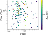 |
Fig. 12 Selection of best targets filtered according to some specific criteria (see Sect. 5.1) obtained from the exoplanet.eu database. The plot shows the planet mass Mpla Vs the distance d for this selection of 124 objects, as well as the planet’s semimajor axis apla in colour. The objects circled in red are those already observed with GRAVITY: AF Lep b, β Pic b, c, HD 1160 b, HD 206893 B, HD 95086 b, HIP 65426 b, HIP 81208 Cb, HIP 99770 b, HR 2562 b, and HR 8799 b, c, d, e. |
K-band magnitude estimates for some potential GRAVITY follow-up targets derived using different evolutionary models: ATMO (Phillips et al. 2020), AMES-DUSTY (Chabrier et al. 2000; Allard et al. 2001), and AMES-COND (Allard et al. 2001; Baraffe et al. 2003).
5.2 The atmospheric makeup
Using cross-correlation, we searched for the presence of different molecules and atoms expected to be present in the atmospheres of brown dwarfs and young giant exoplanets: H2O, CO, CH4, Na, K, HCN, CO2, FeH, H2S, HCN, NH3, PH3, TiO, and VO. For an effective temperature ~1400K, atmospheric models predict spectra dominated by H2O and CO in the K band. We obtained a relatively clear detection of H2O by cross-correlation (S/N~4.1). Surprisingly, the signal is weak for CO (S/N~1.3). In addition to cross-correlation, we performed forward model fitting of the GRAVITY spectrum as described in Sect. 4.1. The best fit (see Fig. C.1) corresponds to C/O=0.38(+0.2/-0.2), slightly subsolar (but note that the posterior is bimodal). This is consistent with the non-detection of CO by cross-correlation.
5.3 Comparison with other methods to detect exomoons
The search for exomoons presents significant challenges and no confirmed detection exists to date. While the transit method (e.g., Kipping et al. 2015; Teachey et al. 2018) and radial velocity techniques (e.g., Ruffio et al. 2023) have driven most exomoon searches, they face inherent limitations. Transit techniques are sensitive primarily to moons on close-in orbits around transiting planets and they require near-perfect orbital alignment, while disentangling moon signals from stellar activity or other planets can be complex. RV techniques require bright stars and struggle to target long-period moons (Ruffio et al. 2023).
High-precision astrometry, as demonstrated in this work with VLTI/GRAVITY, offers a fundamentally complementary pathway. It directly measures the spatial wobble of the host planet or brown dwarf on the sky plane caused by an orbiting moon’s gravitational pull. This technique possesses unique advantages. First, it can target planets with different inclinations, where the transit technique cannot, and the RV technique finds results that depend on the (most frequently) unknown sin(i) value. Second, it is ideally suited for searching for moons around directly imaged substellar companions, which typically reside on wide orbits that are more likely to host moons. Transiting planets have short orbital periods and thus small Hill spheres, which could be less favourable to moon retention (Dobos et al. 2021), even if the planet formed further out and migrated inwards (Spalding et al. 2016). Finally, it is sensitive to wide-orbit moons with periods of months to years, which are inaccessible to transit techniques or current RV sensitivities (Ruffio et al. 2023). Our tentative candidate around HD 206893 B exemplifies this, with a period of ~0.76 years. The astrometry technique is even more powerful for moons at large distances from their planets, whereas the RV semi-amplitude decreases with larger separations, which could be complementary in some cases.
We note that the detection of circumplanetary discs could also help to improve our understanding of the formation sites of exomoons in the near future, which could prove very useful for testing models (e.g., GQ Lup b, Cugno et al. 2024). If cavities are discovered (e.g., with the JWST) in these discs surrounding planets, this could indicate that moons are already forming at an early stage and we could begin to study exomoon formation sites in detail, as well as the materials that accumulate as they form to forge these moons (e.g., Horstman et al. 2024).
5.4 β Pictoris b: Obliquity constraints and exomoon predictions
The young β Pictoris system hosts two directly imaged super-Jupiters (β Pic b and c), offering a prime laboratory for studying planetary dynamics. Upcoming JWST observations (programme GO 4758) will provide the first direct measurement of the spin-orbit obliquity of the outermost planet, β Pic b, establishing a milestone in exoplanet characterization.
Prior to JWST’s definitive constraints, Poon et al. (2024) combined dynamical and observational arguments to assess the likely obliquity of β Pic b. Their analysis strongly favors a misaligned spin axis for the planet. Crucially, the authors propose that this misalignment could be maintained by a secular spin-orbit resonance driven by an unseen exomoon with a minimum mass exceeding Neptune’s (>1 MNep), and orbital period of 3–7 weeks.
Notably, such a companion may be accessible to astrometric detection: Depending on the moon mass (e.g., if it is rather massive and close to ten Neptune masses), the induced astrometric wobble of β Pic b could fall within the capabilities of GRAVITY+. Given the system’s brightness and proximity, we strongly advocate for rapid high-precision astrometric follow-up to test this prediction. A detection would not only validate the resonance mechanism but also provide the first direct evidence of an exomoon sculpting planetary obliquity.
5.5 Misinterpreting a planet for a moon
A fundamental challenge in astrometric exomoon detection is degeneracy: the reflex motion induced in a host planet (or brown dwarf) caused by an unseen planetary-mass companion orbiting the same central star can mimic the astrometric perturbation created by a moon. The astrometric displacement of a moon (see Eq. (5)) is roughly equal to amoonMmoon/Mpla. The signal from a planet would be roughly equal to aplaMpla/M⋆.
Earlier, we found that the astrometric displacement is about 0.0056 au for our set of best-fit parameters for the moon. If it were created by a planet instead, it would mean that aplaMpla/M⋆ ≲ 0.0056 au. One can imagine a massive close-in planet would reproduce this signal, but then it could be detectable using RV. For instance, a planet with a period of 0.76 yr would correspond to a planet with a semimajor axis of about 0.9 au, which would imply a planet mass of ~7 MJup to reproduce the astrometric displacement observed. Such planets can be detected via RV studies. A planet located farther out with a lower mass could also reproduce the signal in some systems with moons at different periods, but then its period will likely be too high compared to typical moon periods, such as the one found here: 0.76 yr. These types of arguments should be checked on a case-by-case basis.
The fundamental difference between the effect of a moon and that of a planet is that the latter will cause a reflex motion on the star, while a moon would not. Hence, a follow-up of the star’s RV would be important to confirm the detection if any doubts remain. For instance, we could explore whether the planet that might be found to mimic the moon’s signal is at the detection limit or whether it is in a system that does not yet have RV limits or strong direct imaging constraints.
6 Conclusions
In this study, we present the first dedicated high-precision astrometric search for an exomoon around a substellar companion, HD 206893 B, using VLTI/GRAVITY. Our analysis of the companion’s orbital motion revealed an upper limit of 0.8 MJup and possible tentative astrometric residuals consistent with a perturbation potentially induced by an exomoon. If confirmed, this signal would correspond to a massive satellite (~0.5 MJup) orbiting HD 206893 B with a period of approximately 0.76 years. We emphasize the tentative nature of this candidate, which would require further confirmation using GRAVITY data.
Beyond the exomoon signature, our work significantly refines the architecture of the HD 206893 system. Re-fitting the orbits of companions B and c suggests HD 206893 B resides on a wider orbit (10.75±0.08 au) than previously estimated, implying a lower mass for this object (![Mathematical equation: $\[19.5_{-1.3}^{+1.4}\]$](/articles/aa/full_html/2026/01/aa57127-25/aa57127-25-eq43.png) MJup). This revision may impact our understanding of the system’s formation and dynamical history.
MJup). This revision may impact our understanding of the system’s formation and dynamical history.
Complementing the astrometry, we analyzed the R = 4000 spectrum of HD 206893 B obtained with GRAVITY, confirming a clear detection of water, and no CO detection. These spectral features provide crucial insights into the atmospheric composition and physical properties of this substellar companion.
Looking beyond HD 206893, we identified the most promising targets for future astrometric exomoon searches with GRAVITY. Based on proximity, companion brightness (K-band magnitude), orbital characteristics, and predicted astrometric signal strength, the five optimal candidates are: AF Lep b, HD 155555 (AB) b, β Pic b, HD 60584 b, and 2MASS J1315-2649 b. Here, a priority is attributed to AF Lep b and β Pic b that can be observed without further characterization of the orbits, which are sufficiently well known to follow them precisely with GRAVITY+. These systems present the strongest prospects for detecting the tens of μas astrometric wobbles induced by exomoons within the current capabilities of VLTI/GRAVITY.
Our results demonstrate the potential of high-precision astrometry in the search for exomoons. While the detection around HD 206893 B requires further validation, this study establishes the methodology and proves the feasibility of the technique in addition to the analytical work by Winterhalder et al. (2026). GRAVITY, designed with the hope to reach micro-arcsecond precision (Lacour et al. 2014), is currently the only instrument capable of pursuing this astrometric pathway to Neptune-like exomoons around directly imaged exoplanets and substellar companions. We therefore conclude that VLTI/GRAVITY has a pivotal role to play in the emerging field of exomoon and binary planet discovery. Future observations focusing on the HD 206893 system and the prioritized target list are essential to confirm the first exomoon and to usher in a new era of comparative exolunar science. New instruments at the VLTI with greater astrometric precision (e.g., Lacour et al. 2025) or a future kilometer baseline interferometric facility would allow us to reach 1 μas (Bourdarot & Eisenhauer 2024), which would push the detection limits down by more than an order of magnitude.
Acknowledgements
This paper is dedicated to Rémi. We thank the referee for their thorough report that improved the paper substantially. Based on observations collected at the European Southern Observatory under ESO programmes 105.20T0.001, 109.22ZA.002, 1103.B-0626, 1104.C-0651, 113.26D9.001 and 114.27UV.001. This research has made use of the Jean-Marie Mariotti Center Aspro service. J.S-B. acknowledges the support received by the UNAM DGAPA-PAPIIT project AG-101025 and from the SECIHTI Ciencia de Frontera project CBF-2025-I-3033. S.L. acknowledges the support of the French Agence Nationale de la Recherche (ANR-21-CE31-0017, ExoVLTI) and of the European Union (ERC Advanced Grant 101142746, PLANETES). P.K. acknowledges funding from the European Research Council (ERC) under the European Union’s Horizon 2020 research and innovation program (project UniverScale, grant agreement 951549).
References
- Allard, F., & Homeier, D., 2012, in EAS Publications Series, 57, eds. C. Reylé, C. Charbonnel, & M. Schultheis, Low-Mass Stars and the Transition Stars/Brown Dwarfs: Atmospheres from Very Low-Mass Stars to Extrasolar Planets (Les Ulis: EDP Sciences), 3 [Google Scholar]
- Allard, F., Hauschildt, P. H., Alexander, D. R., Tamanai, A., & Schweitzer, A. 2001, ApJ, 556, 357 [Google Scholar]
- Allard, F., Homeier, D., & Freytag, B. 2012, RSPTA, 370, 2765 [Google Scholar]
- Asensio-Torres, R., Janson, M., Bonavita, M., et al. 2018, A&A, 619, A43 [NASA ADS] [CrossRef] [EDP Sciences] [Google Scholar]
- Balmer, W. O., Franson, K., Chomez, A., et al. 2025, AJ, 169, 30 [NASA ADS] [Google Scholar]
- Baraffe, I., Chabrier, G., Barman, T. S., Allard, F., & Hauschildt, P. H. 2003, A&A, 402, 701 [NASA ADS] [CrossRef] [EDP Sciences] [Google Scholar]
- Batygin, K., & Morbidelli, A. 2020, ApJ, 894, 143 [NASA ADS] [CrossRef] [Google Scholar]
- Blain, D., Charnay, B., & Bézard, B. 2021, A&A, 646, A15 [EDP Sciences] [Google Scholar]
- Blunt, S., Wang, J. J., Angelo, I., et al. 2020, AJ, 159, 3, 89 [NASA ADS] [CrossRef] [Google Scholar]
- Blunt, S., Wang, J., Hirsch, L., et al. 2024, J. Open Source Softw., 9, 6756 [Google Scholar]
- Bonavita, M., Fontanive, C., Gratton, R., et al. 2022, MNRAS, 513, 5588 [NASA ADS] [Google Scholar]
- Bourdarot, G., & Eisenhauer, F. 2024, arXiv doi:10.48550/arXiv.2410.22063 [Google Scholar]
- Bourdarot, G., Eisenhauer, F., Yazıcı, S., et al. 2024, arXiv doi:10.48550/arXiv.2409.08438 [Google Scholar]
- Brandt, T. D. 2021, ApJS, 254, 42 [NASA ADS] [CrossRef] [Google Scholar]
- Burgasser, A. J., Sitarski, B. N., Gelino, C. R., Logsdon, S. E., & Perrin, M. D. 2011, ApJ, 739, 49 [NASA ADS] [CrossRef] [Google Scholar]
- Carrasco, J. M., Weiler, M., Jordi, C., et al. 2021, A&A, 652, A86 [NASA ADS] [CrossRef] [EDP Sciences] [Google Scholar]
- Chabrier, G., Baraffe, I., Allard, F., & Hauschildt, P. 2000, ApJ, 542, 464 [Google Scholar]
- Chandrasekhar, S. 1969, efe..book [Google Scholar]
- Charnay, B., Bézard, B., Baudino, J.-L., et al. 2018, ApJ, 854, 172 [Google Scholar]
- Cugno, G., Patapis, P., Banzatti, A., et al. 2024, ApJ, 966, L21 [NASA ADS] [CrossRef] [Google Scholar]
- Cutri, R. M., Skrutskie, M. F., van Dyk, S., et al. 2003, yCat, 2246, II/246 [Google Scholar]
- De Angeli, F., Weiler, M., Montegriffo, P., et al. 2023, A&A, 674, A2 [NASA ADS] [CrossRef] [EDP Sciences] [Google Scholar]
- de Regt, S., Gandhi, S., Snellen, I. A. G., et al. 2024, A&A, 688, A116 [NASA ADS] [CrossRef] [EDP Sciences] [Google Scholar]
- Delorme, P., Schmidt, T., Bonnefoy, M., et al. 2017, A&A, 608, A79 [NASA ADS] [CrossRef] [EDP Sciences] [Google Scholar]
- Dencs, Z., Dobos, V., & Regály, Z. 2025, A&A, 699, A166 [NASA ADS] [CrossRef] [EDP Sciences] [Google Scholar]
- Dobos, V., Charnoz, S., Pál, A., Roque-Bernard, A., & Szabó, G. M. 2021, PASP, 133, 094401 [NASA ADS] [CrossRef] [Google Scholar]
- Domingos, R. C., Winter, O. C., & Yokoyama, T. 2006, MNRAS, 373, 1227 [NASA ADS] [CrossRef] [Google Scholar]
- Foreman-Mackey, D., Hogg, D. W., Lang, D., et al. 2013, PASP, 125, 306 [NASA ADS] [CrossRef] [Google Scholar]
- Franson, K., Bowler, B. P., Zhou, Y., et al. 2023, ApJ, 950, L19 [NASA ADS] [CrossRef] [Google Scholar]
- Gaia Collaboration 2018, yCat, 1345, doi:10.26093/cds/vizier.1345 [Google Scholar]
- Gaia Collaboration 2020, yCat, 1350, doi:10.26093/cds/vizier.1350 [Google Scholar]
- Gaia Collaboration (Vallenari, A., et al.) 2023, A&A, 674, A1 [NASA ADS] [CrossRef] [EDP Sciences] [Google Scholar]
- Grandjean, A., Lagrange, A.-M., Beust, H., et al. 2019, A&A, 627, L9 [NASA ADS] [CrossRef] [EDP Sciences] [Google Scholar]
- Gratton, R., Mesa, D., Bonavita, M., et al. 2023, NatCo, 14, 6232 [Google Scholar]
- GRAVITY Collaboration (Abuter, R., et al.) 2017, A&A, 602, A94 [NASA ADS] [CrossRef] [EDP Sciences] [Google Scholar]
- GRAVITY Collaboration (Nowak, M., et al.) 2020, A&A, 633, A110 [NASA ADS] [CrossRef] [EDP Sciences] [Google Scholar]
- GRAVITY Collaboration (Abuter, R., et al.) 2021, A&A, 647, A59 [NASA ADS] [CrossRef] [EDP Sciences] [Google Scholar]
- Han, C., & Han, W. 2002, ApJ, 580, 490 [NASA ADS] [CrossRef] [Google Scholar]
- Hansen, B. M. S. 2019, SciA, 5, eaaw8665 [Google Scholar]
- Heller, R., Rodenbeck, K., & Bruno, G. 2019, A&A, 624, A95 [NASA ADS] [CrossRef] [EDP Sciences] [Google Scholar]
- Heller, R., & Hippke, M. 2024, NatAs, 8, 193 [Google Scholar]
- Hinkley, S., Lacour, S., Marleau, G.-D., et al. 2023, A&A, 671, L5 [NASA ADS] [CrossRef] [EDP Sciences] [Google Scholar]
- Horstman, K., Ruffio, J.-B., Batygin, K., et al. 2024, AJ, 168, 175 [Google Scholar]
- Kammerer, J., Lacour, S., Stolker, T., et al. 2021, A&A, 652, A57 [NASA ADS] [CrossRef] [EDP Sciences] [Google Scholar]
- Kipping, D. M. 2009, MNRAS, 392, 181 [NASA ADS] [CrossRef] [Google Scholar]
- Kipping, D. M. 2009, MNRAS, 396, 1797 [NASA ADS] [CrossRef] [Google Scholar]
- Kipping, D. M., Schmitt, A. R., Huang, X., et al. 2015, ApJ, 813, 14 [NASA ADS] [CrossRef] [Google Scholar]
- Konopacky, Q. M., Barman, T. S., Macintosh, B. A., & Marois, C. 2013, Science, 339, 1398 [Google Scholar]
- Kipping, D., Bryson, S., Burke, C., et al. 2022, NatAs, 6, 367 [Google Scholar]
- Kral, Q., Schneider, J., Kennedy, G., & Souami, D. 2016, A&A, 592, A39 [NASA ADS] [CrossRef] [EDP Sciences] [Google Scholar]
- Kreidberg, L., Luger, R., & Bedell, M. 2019, ApJ, 877, L15 [NASA ADS] [CrossRef] [Google Scholar]
- Lacour, S., Eisenhauer, F., Gillessen, S., et al. 2014, A&A, 567, A75 [NASA ADS] [CrossRef] [EDP Sciences] [Google Scholar]
- Lacour, S., Wang, J. J., Nowak, M., et al. 2020, SPIE, 11446, 1144600 [Google Scholar]
- Lacour, S., Wang, J. J., Rodet, L., et al. 2021, A&A, 654, L2 [NASA ADS] [CrossRef] [EDP Sciences] [Google Scholar]
- Lacour, S., Carrión-González, Ó., & Nowak, M. 2025, A&A, 694, A277 [NASA ADS] [CrossRef] [EDP Sciences] [Google Scholar]
- Lagrange, A.-M., Bonnefoy, M., Chauvin, G., et al. 2010, Science, 329, 57 [Google Scholar]
- Lapeyrere, V., Kervella, P., Lacour, S., et al. 2014, SPIE, 9146, 91462D [Google Scholar]
- Lazzoni, C., Zurlo, A., Desidera, S., et al. 2020, A&A, 641, A131 [NASA ADS] [CrossRef] [EDP Sciences] [Google Scholar]
- Liddle, A. R. 2007, MNRAS, 377, L74 [NASA ADS] [Google Scholar]
- Limbach, M. A., Vos, J. M., Winn, J. N., et al. 2021, ApJ, 918, L25 [CrossRef] [Google Scholar]
- Marino, S., Zurlo, A., Faramaz, V., et al. 2020, MNRAS, 498, 1319 [Google Scholar]
- Milli, J., Hibon, P., Christiaens, V., et al. 2017, A&A, 597, L2 [NASA ADS] [CrossRef] [EDP Sciences] [Google Scholar]
- Moraes, R. A., & Vieira Neto, E. 2020, MNRAS, 495, 3763 [CrossRef] [Google Scholar]
- Murray, C. D., & Dermott, S. F. 1999, ssd..book. doi:10.1017/CB09781139174817 [Google Scholar]
- Petrus, S., Chauvin, G., Bonnefoy, M., et al. 2025, A&A, 701, A208 [NASA ADS] [CrossRef] [EDP Sciences] [Google Scholar]
- Poon, M., Rein, H., & Pham, D. 2024, OJAp, 7, 109 [Google Scholar]
- Porco, C. C., Thomas, P. C., Weiss, J. W., & Richardson, D. C. 2007, Science, 318, 1602 [NASA ADS] [CrossRef] [Google Scholar]
- Phillips, M. W., Tremblin, P., Baraffe, I., et al. 2020, A&A, 637, A38 [NASA ADS] [CrossRef] [EDP Sciences] [Google Scholar]
- Roche, É., 1849, in Académie des Sciences Montpellier: Mémoires la Section des Sciences, 1, 243 [Google Scholar]
- Ruffio, J.-B., Horstman, K., Mawet, D., et al. 2023, AJ, 165, 113 [NASA ADS] [CrossRef] [Google Scholar]
- Sappey, B., Konopacky, Q., Ó C. R. D., et al. 2025, AJ, 169, 175 [Google Scholar]
- Sartoretti, P., & Schneider, J. 1999, A&AS, 134, 553 [NASA ADS] [CrossRef] [EDP Sciences] [Google Scholar]
- Schneider, J., Dedieu, C., Le Sidaner, P., Savalle, R., & Zolotukhin, I. 2011, A&A, 532, A79 [NASA ADS] [CrossRef] [EDP Sciences] [Google Scholar]
- Simon, A., Szatmáry, K., & Szabó, G. M. 2007, A&A, 470, 727 [NASA ADS] [CrossRef] [EDP Sciences] [Google Scholar]
- Spalding, C., Batygin, K., & Adams, F. C. 2016, ApJ, 817, 18 [Google Scholar]
- Stern, S. A., & Levison, H. F. 2002, HiA, 12, 205 [Google Scholar]
- Stolker T., 2023, ascl.soft. [record ascl:2307.057] [Google Scholar]
- Teachey, A., & Kipping, D. M. 2018, SciA, 4, eaav1784 [Google Scholar]
- Teachey, A., Kipping, D. M., & Schmitt, A. R. 2018, AJ, 155, 36 [Google Scholar]
- Vanderburg, A., & Rodriguez, J. E. 2021, ApJ, 922, L2 [NASA ADS] [CrossRef] [Google Scholar]
- Vanderburg, A., Rappaport, S. A., & Mayo, A. W. 2018, AJ, 156, 184 [NASA ADS] [CrossRef] [Google Scholar]
- Vousden, W. D., Farr, W. M., & Mandel, I. 2016, MNRAS, 455, 1919 [NASA ADS] [CrossRef] [Google Scholar]
- Ward-Duong, K., Patience, J., Follette, K., et al. 2021, AJ, 161, 5 [Google Scholar]
- Winterhalder, T. O., Mérand, A., Kammerer, J., et al. 2026, A&A, 705, A216 [NASA ADS] [CrossRef] [EDP Sciences] [Google Scholar]
Available for download at https://gitlab.obspm.fr/mnowak/exogravity
Appendix A Spectral data at different epochs
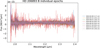 |
Fig. A.1 Individual (color) spectra obtained with GRAVITY for HD 206893 B at the dates indicated in the figure’s legend. The legend further reveals the best fitting scale factor for each epoch (see Sect. 2 for details) and that all epochs were observed in dual-field on-axis mode. |
Appendix B Orbital fit while fixing the semimajor axis of the moon
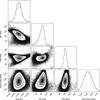 |
Fig. B.1 Fit of the astrometric data of HD 206893 B, looking for an exomoon when we limited the prior to be between 0.21 and 0.26 au. The MCMC analysis finds a tentative exomoon candidate of mass around 0.5 Jupiter masses. |
Appendix C Bayesian analysis of the atmospheric spectrum of HD 206893 B
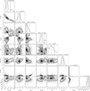 |
Fig. C.1 Posterior distributions obtained from Bayesian forward modeling of HD 206893 B’s atmospheric spectrum with ExoREM, displayed in a corner plot. |
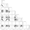 |
Fig. C.2 Posterior distributions obtained from Bayesian forward modeling of HD 206893 B’s atmospheric spectrum with ATMO, displayed in a corner plot. |
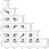 |
Fig. C.3 Posterior distributions obtained from Bayesian forward modeling of HD 206893 B’s atmospheric spectrum with BT-Settl, displayed in a corner plot. |
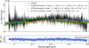 |
Fig. C.4 Best fit models overlaid on GRAVITY data for the forward modeling of the atmospheric spectrum of HD 206893 B using a Bayesian framework (upper panel). Residuals with ExoREM model are presented as an example (bottom panel). |
Appendix D Log of all GRAVITY observations
Observation log for HD206893
Astrometry as a function of time and polynomial order.
All Tables
K-band magnitude estimates for some potential GRAVITY follow-up targets derived using different evolutionary models: ATMO (Phillips et al. 2020), AMES-DUSTY (Chabrier et al. 2000; Allard et al. 2001), and AMES-COND (Allard et al. 2001; Baraffe et al. 2003).
All Figures
|
Fig. 1 Schematic of the HD 206893 system. |
| In the text | |
|
Fig. 2 Model spectrum of HD 206893 A obtained by fitting a BT-NextGen stellar model atmosphere (black line) to archival photometry (orange points) and the Gaia XP spectrum (green points). The top panel shows the filter transmission curves and the bottom panel shows the residuals between the data and model. |
| In the text | |
|
Fig. 3 Combined R ~ 4000 spectrum obtained with GRAVITY for HD 206893 B by averaging the data obtained at different epochs (see Fig. A.1). |
| In the text | |
|
Fig. 4 Diagram of the orbit of HD 206893 B with a potential moon around it, causing it to shift slightly due to the moon’s gravitational potential. It illustrates the notation used in Sect. 3.1. |
| In the text | |
|
Fig. 5 Analytical predictions of Mmoon (the mass of the moon in masses of Neptune) as a function of Tmoon (the period of the moon in days). The solid black lines show the model’s prediction for astrometric accuracies of 10 and 100 μas, as indicated on the graph. The values used are those of Eq. (6), i.e., d = 10 pc and Mpla = 10 MJup. The dotted line shows the case of 10 μas considering Mpla = 1 MJup. If the system is instead at 100 pc, the lines are pushed up by a factor of 10. The areas beyond the Roche limit and the Hill sphere are shown in grey. The Hill sphere is shown for two values of the semimajor axis of the planet apla equal to 1 (closest) and 10 au (farthest). The horizontal lines indicate moon masses of 1 MJup, 1 MNep, 1 M⊕, and 1 MGanymede from top to bottom. |
| In the text | |
|
Fig. 6 Analytical predictions for the astrometric effect of a moon with varying mass and distance to HD 206893 B. GRAVITY could in principle detect moons lower than a Neptune mass at larger periods. The fit of the GRAVITY data is shown as a green point assuming the mass and period as upper limits in our tentative detection. The orange area shows the plausible parameter space where a moon might be located, and still be potentially detectable with GRAVITY assuming an astrometric accuracy of 10 μas (see Sect. 3.3). |
| In the text | |
|
Fig. 7 Fit of the astrometric data of HD 206893 B looking for an exomoon. The MCMC analysis finds a 95% upper limit of 0.8 MJup for the potential exomoon mass and a peak in semimajor axis at 0.22 au, while the inclination and position angle of ascending node are around 90 deg. Another MCMC plot assuming a fixed semimajor axis around its peak is shown in Fig. B.1. |
| In the text | |
|
Fig. 8 Residuals of HD 206893 B orbit after removing the average motion due to HD 206893 B orbiting the star and accounting for the motion induced by the planet c. In the top two plots, the data are phase-folded by a period of 275 days, using MJD 58500 as the starting point. 50 random draws with SMA between 0.21 and 0.26 AU are plotted in cyan for the RA and orange for the Dec Vs time plots, respectively. These model draws have the average motion of HD 206893 B removed, so they show both perturbation from the exomoon model and the residuals in the orbit of B from the average orbit of B. In the bottom plots, the data are plotted as a function of MJD and not phase-folded. The orbits are colored by orbital phase, where blue is an orbital phase of 0 and green is an orbital phase of 1. Note: the orbital periods vary between each model drawn and are slightly different from an exact 275-day orbital period. |
| In the text | |
|
Fig. 9 Similar residuals as Fig. 8, but projected onto the 2-D sky plane and the 50 random draws from the posterior only consider the motion of a potential exomoon (and not residual uncertainties in the orbit of B, which are shown in Fig. 8). The colors of both the data and the models correspond to the 275-day phase, as specified by the colorbar and defined in Fig. 8. |
| In the text | |
|
Fig. 10 Comparison between the GRAVITY combined spectrum (gray) and the ExoREM synthetic spectrum for T = 1400 K (light blue). Each species spectrum is shown with an offset with different colours – dark blue for water, pink for sodium, and red for CO. |
| In the text | |
|
Fig. 11 Cross-correlation S/N peaks between the data and the ExoREM synthetic spectrum for T = 1400 K. The global cross-correlation S/N are computed as the peak divided by the standard deviation of the CCF wings (500 to 3000 km/s), with their final values displayed in the legend for each species (in colour) and for the global atmospheric model (in black). |
| In the text | |
|
Fig. 12 Selection of best targets filtered according to some specific criteria (see Sect. 5.1) obtained from the exoplanet.eu database. The plot shows the planet mass Mpla Vs the distance d for this selection of 124 objects, as well as the planet’s semimajor axis apla in colour. The objects circled in red are those already observed with GRAVITY: AF Lep b, β Pic b, c, HD 1160 b, HD 206893 B, HD 95086 b, HIP 65426 b, HIP 81208 Cb, HIP 99770 b, HR 2562 b, and HR 8799 b, c, d, e. |
| In the text | |
|
Fig. A.1 Individual (color) spectra obtained with GRAVITY for HD 206893 B at the dates indicated in the figure’s legend. The legend further reveals the best fitting scale factor for each epoch (see Sect. 2 for details) and that all epochs were observed in dual-field on-axis mode. |
| In the text | |
|
Fig. B.1 Fit of the astrometric data of HD 206893 B, looking for an exomoon when we limited the prior to be between 0.21 and 0.26 au. The MCMC analysis finds a tentative exomoon candidate of mass around 0.5 Jupiter masses. |
| In the text | |
|
Fig. C.1 Posterior distributions obtained from Bayesian forward modeling of HD 206893 B’s atmospheric spectrum with ExoREM, displayed in a corner plot. |
| In the text | |
|
Fig. C.2 Posterior distributions obtained from Bayesian forward modeling of HD 206893 B’s atmospheric spectrum with ATMO, displayed in a corner plot. |
| In the text | |
|
Fig. C.3 Posterior distributions obtained from Bayesian forward modeling of HD 206893 B’s atmospheric spectrum with BT-Settl, displayed in a corner plot. |
| In the text | |
|
Fig. C.4 Best fit models overlaid on GRAVITY data for the forward modeling of the atmospheric spectrum of HD 206893 B using a Bayesian framework (upper panel). Residuals with ExoREM model are presented as an example (bottom panel). |
| In the text | |
Current usage metrics show cumulative count of Article Views (full-text article views including HTML views, PDF and ePub downloads, according to the available data) and Abstracts Views on Vision4Press platform.
Data correspond to usage on the plateform after 2015. The current usage metrics is available 48-96 hours after online publication and is updated daily on week days.
Initial download of the metrics may take a while.