| Issue |
A&A
Volume 705, January 2026
|
|
|---|---|---|
| Article Number | A111 | |
| Number of page(s) | 9 | |
| Section | Stellar atmospheres | |
| DOI | https://doi.org/10.1051/0004-6361/202557325 | |
| Published online | 12 January 2026 | |
Deciphering transmission spectra by exploring the solar paradigm
1
Institut de Ciències de l’Espai (ICE, CSIC),
Campus UAB, c/ Can Magrans s/n, 08193 Bellaterra,
Barcelona,
Spain
2
Institut d’Estudis Espacials de Catalunya (IEEC),
Edifici RDIT, Campus UPC,
08860
Castelldefels (Barcelona),
Spain
3
Institut für Physik, Universität Graz,
Universitätsplatz 5/II,
8010
Graz,
Austria
4
Max-Planck-Institut für Sonnensystemforschung
Justus-von-Liebig-Weg 3,
37077
Göttingen,
Germany
★ Corresponding author: This email address is being protected from spambots. You need JavaScript enabled to view it.
Received:
19
September
2025
Accepted:
7
December
2025
Abstract
Aims. Transmission spectroscopy allows to measure the wavelength dependence of the transit signal of an exoplanet, thus enabling probing of its atmospheric composition. However, the transmission spectrum also carries information of the host star, generally referred to as ‘contamination‘. Stellar activity leads to an apparent change in the stellar radius, directly impacting the transit depth. This contamination is regarded as the major hurdle in discovering and characterising the atmospheres of exoplanets.
Methods. The objective is to understand how the chromatic effect (i.e. the wavelength dependence) of the stellar activity-induced transit depth depends on the surface distribution of magnetic features. The surface distribution of other stars generally is unknown, with the exception of our very own star, the Sun. We therefore investigate the solar paradigm as ‘ground truth’ to explore how much the chromatic effects depends on the distribution of magnetic features. In particular, we explored the impact of centre-to-limb variations (CLV) of the magnetic features and their resulting chromatic effect. Specifically, we investigated the solar paradigm as the ‘ground truth’.
Results. We utilised spot and faculae masks obtained from SDO/HMI magnetograms and intensitygrams together with the SATIRE approach of calculating solar variability to calculate the chromatic dependence of the apparent radius of the Sun for the last solar cycle. We tested several approaches to convolving the area coverage with the spectra to uncover the potential biases and we investigated the drivers responsible for the chromatic effect.
Conclusions. We find that using a simplified approach that only relies on the disc area coverage and neglects CLV in the spectra to calculate the chromatic effects lead to an underestimation of the apparent radius. In particular, for the faculae component, the CLV need to be taken into account accordingly, especially since the facular area coverage is by far larger than that of spots for stars with near-solar activity level. We report that this chromatic dependence can be detected in transits of an Earth-sized and a Jupiter-sized planet. Additionally, we assessed the amplitude of this effect between solar minimum and solar maximum. We found that for a Jupiter-like transit this amplitude is at the level of 40 ppm, well above the 10 ppm noise floor of JWST. However, this effect is only on the level of 0.4 ppm for the Earth-like transit.
Key words: Sun: atmosphere / Sun: faculae, plages / Sun: magnetic fields / sunspots / stars: atmospheres / stars: low-mass
© The Authors 2026
 Open Access article, published by EDP Sciences, under the terms of the Creative Commons Attribution License (https://creativecommons.org/licenses/by/4.0), which permits unrestricted use, distribution, and reproduction in any medium, provided the original work is properly cited.
This article is published in open access under the Subscribe to Open model. This email address is being protected from spambots. You need JavaScript enabled to view it. to support open access publication.
1 Introduction
Exoplanet research has advanced tremendously since the first detection of an exoplanet around a star similar to our Sun (Mayor & Queloz 1995). Methods have been developed to allow for the detection of small rocky planets and, in parallel, techniques for the characterisation of exoplanetary atmospheres have also been established. The most powerful technique for studying and characterising the atmospheres of exoplanets at present is transmission spectroscopy (Seager & Sasselov 2000; Charbonneau et al. 2002; Tinetti et al. 2007; Yan et al. 2019; Rustamkulov et al. 2023). The planet will appear larger at wavelengths where the atmosphere is more opaque, which, in turn, depends on its chemical composition. Thus, by studying the dependence of the depth of the planetary transit on the wavelength (i.e. the transmission spectrum), information on the abundances of relevant chemical compounds can be obtained. On the other hand, the star’s apparent radius can also vary with wavelength Seager & Shapiro (2024), particularly if it exhibits magnetic activity. This is manifested as dark or bright regions on its surface Solanki et al. (see 2013, for a review on magnetically driven stellar activity).
Technical efforts to detect and characterise Earth-like planets have pushed the capabilities of our instruments to the detection limit of such planets and the remaining hurdle is the stellar signal (Rackham et al. 2023). While the signal itself provides precious information of the star, its activity in particular, it is often seen as ‘noise’ plaguing efforts to retrieve the planetary characteristics. The stellar activity signal can have different sources, depending on the timescales considered. Most prominently, it is the stellar magnetic activity on cool stars, such as our Sun, manifesting itself in in the form of bright and dark regions (generally referred to as spot and faculae) on stellar surfaces (Solanki et al. 2013; Ermolli et al. 2013). Whilst spot or faculae crossings can be seen in the individual transit light curves (for instance Petit dit de la Roche et al. 2024; Ahrer et al. 2025; Fournier-Tondreau et al. 2025; Radica et al. 2025), unocculted features pose further threats to the reliable characterisation of planetary atmospheres.
While there are some promising attempts underway to correct for stellar activity contamination from the transmission spectrum (i.e. leveraging contemporaneous multi-technique observations Mallonn et al. 2018; Rosich et al. 2020 or machine learning approaches Ardévol Martínez et al. 2022; Matchev et al. 2022; Lueber et al. 2024), we still largely rely on forward models of stellar activity. In such models, a rotating stellar photosphere is filled with magnetic features (spots and faculae; see e.g. Rackham et al. 2019, for a general overview of the approach). Usually, a grid of models, with varying active region coverage and configurations, as well as temperature contrasts of the features with respect to the quiet photosphere, is generated. Then, iteratively, models from such a grid are fitted to the observed wavelength-dependent light curves. After the best fit model is found, this chromatic stellar model is removed from the observed transmission spectrum to remove the stellar contamination (f.i. Lim et al. 2023; Radica et al. 2025). The stellar radius (or, rather, the star-to-planet radius ratio, with the radii being squared, respectively) is often also considered a free parameters in the fitting. In short, forward models rely on two components: the spectra of magnetic features and the quiet stellar surface, and their spatial distribution of the surface of the star. A lot of effort has been put into improving the fidelity of of spectra for the magnetic activity components (Witzke et al. 2022). Rosich et al. (2020) have shown that the same projected area coverage, but different configurations of magnetic features lead to different contaminations in the transmission spectrum. This raises the question, how well constrained the magnetic feature distribution has to be in order to remove the contamination, or if there is some leeway. As the distribution of magnetic features on other stars is unknown, we chose to focus on the only star for which this is known: the Sun. To this end, we utilise the observed distribution of magnetic features of the Sun by using spot and facula masks obtained from SDO/HMI images and magnetograms. These features are then weighted with their corresponding spectra taken from Unruh et al. (1999). We then followed the approach of Seager & Shapiro (2024) to calculate the apparent radius of the star, in our case the Sun, and compare this to a star that would be free of magnetic features. This way, we model the effect that un-occulted features have on the transmission spectrum of a planet. We introduce the model in more detail in Sect. 2. The apparent radius change and its causes are discussed in Sect. 3. We conclude the paper and its is limitations to use for other stars in Sect. 4.
2 Model
The transit depth, T D(λ) induced by a transiting planet generally is written as
 (1)
with R(λ)p being the radius of the planet and R(λ)* the apparent radius of the star. The apparent size of the star is varying with time due to the presence of magnetic features; in the presence of a large spot, the stellar radius appears to ‘shrink’ (the spot temperature is cooler than the non-magnetic photosphere; hence the measured effective temperature is cooler than the photospheric effective temperature). Therefore, we can rewrite
(1)
with R(λ)p being the radius of the planet and R(λ)* the apparent radius of the star. The apparent size of the star is varying with time due to the presence of magnetic features; in the presence of a large spot, the stellar radius appears to ‘shrink’ (the spot temperature is cooler than the non-magnetic photosphere; hence the measured effective temperature is cooler than the photospheric effective temperature). Therefore, we can rewrite  as
as  with A denoting a star with some level of magnetic activity. We stress once again that the apparent radius in Eq. (1) is only due to the presence of stellar activity and not a physical change in the radius of the star (as induced by e.g. oscillations).
Following Seager & Shapiro (2024) and taking into account that we are only concerned with the Sun in the following, we use ⊙ instead of ★ and write the apparent solar radius  as
as
 (2)
where
(2)
where  denotes the apparent solar radius in the presence of magnetic features on the surface,
  denotes the ‘quiet’ (i.e. a Sun that is free of magnetic features) solar radius, αi is the fractional coverage by the considered magnetic feature i (either a spot or facula), F(λ)i is the flux of the given feature, and F(λ)Q is the quiet Sun flux. As discussed in Seager & Shapiro (2024), the approach in Eq. (2) does not take into account centre-to-limb variations (CLV) in the spectra and the area coverage αi represents the disc area coverage, neglecting the actual distribution of the features.
Our ‘ground truth’ approach utilises the observed distribution of the magnetic features (in the present study faculae and spots), which is obtained following Yeo et al. (2014) using images from the Helioseismic and Magnetic Imager onboard the Solar Dynamics Observatory (SDO/HMI Schou et al. 2012) spanning from 2010 May to 2021 January. Following the Spectral And Total Irradiance REconstruction (SATIRE Fligge et al. 2000; Krivova et al. 2003) approach, we introduce the facular saturation threshold (which determines the area coverage from spot corrected HMI magnetograms), Bsat. Here, Bsat is the only free parameter in the model. Since the magnetic elements that form faculae are too small to be resolved in the full-disc HMI magnetograms, we assumed that the facular filling factor increases linearly with increasing magnetic flux up to a saturation point, Bsat, above which the pixel is assumed to be filled fully by faculae and the filling factor is set equal to unit (Ball et al. 2012). We used Bsat=305 G, as discussed in Kopp et al. (2024). We utilised one image per day (if available) and each image represents a 12 minute average. This gives us enough coverage to capture the day-to-day variability of the solar activity, which is primarily driven by magnetic activity (Solanki et al. 2013; Ermolli et al. 2013; Shapiro et al. 2017). Therefore, we rewrote Eq. (2) to take into account the fractional area by spots and faculae and their position-dependent flux in each pixel of HMI images with coordinates, m, n,
 (3)
For each of the magnetic components, we utilised the commonly used 1D fluxes for quiet Sun, spot (divided in umbra and penumbra) and faculae computed by Castelli & Kurucz (1994); Unruh et al. (1999) with the use of the spectral synthesis code ATLAS9 (Kurucz 1992). To take CLV into account, those fluxes are calculated at ten different μ-positions on the solar disc, where μ = cos (θ) (θ is the angle between the observer’s direction and the position vector defined with respect to the centre of the Sun. We limit ourselves to the wavelength regime from 0.6 to 6 μm, covering the wavelength regimes of the JWST NIRSpec (Jakobsen et al. 2022; Böker et al. 2022) instrument, while preserving the original resolution of the spectra. To investigate the importance of both the distribution of magnetic features and their contrasts, we utilised the previously introduced calculations of the apparent radius and denote the approaches in the following way,
(3)
For each of the magnetic components, we utilised the commonly used 1D fluxes for quiet Sun, spot (divided in umbra and penumbra) and faculae computed by Castelli & Kurucz (1994); Unruh et al. (1999) with the use of the spectral synthesis code ATLAS9 (Kurucz 1992). To take CLV into account, those fluxes are calculated at ten different μ-positions on the solar disc, where μ = cos (θ) (θ is the angle between the observer’s direction and the position vector defined with respect to the centre of the Sun. We limit ourselves to the wavelength regime from 0.6 to 6 μm, covering the wavelength regimes of the JWST NIRSpec (Jakobsen et al. 2022; Böker et al. 2022) instrument, while preserving the original resolution of the spectra. To investigate the importance of both the distribution of magnetic features and their contrasts, we utilised the previously introduced calculations of the apparent radius and denote the approaches in the following way,
Approach 1: Utilising Eq. (2) and calculating the mean over the μ-positions of the given spectra, namely, F(λ)= ∫ F(λ, μ) dμ F(λ)=〈 F(λ, μ)〉disc;
Approach 2: Utilising Eq. (3), representing the ‘ground truth’ in the present work.
We remark that the calculations presented below correspond to chromatic dependencies that would occur in the transmission spectrum of a planet that does not cross any magnetic feature (i.e. the transmission spectrum contaminated by un-occulted features). The scaling relations presented later in this work therefore can be used as a template to correct for un-occulted features in the transmission spectra.
The outlined approaches for calculating the activity-induced apparent stellar radius due to stellar activity differ in the type of spectra considered. Approach 1, using F(λ)=∫ F(λ, μ) dμ, corresponds to a solid-angle weighted average disc integrated spectrum. In approach 2, which we treat in the following as the ground truth, represents the most accurate description of the apparent solar radius by taking into account the distribution of the magnetic features and their respective spectra properly.
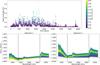 |
Fig. 1 Dependence of the apparent solar radius as a function of solar activity for the different approaches. Top: spot area coverage as a function of the time for solar cycle 24. The spot disc area coverage is shown in different colours. Bottom: approach 1 corresponds to the disc integrated spectra and approach 2 takes the spectra of each pixel of the HMI maps into account. |
3 Results
3.1 Activity induced solar apparent radius change
In Fig. 1, we show the results of the calculations with the different approaches outlined above. The top panel displays the spot area coverage (our chosen activity indicator) as a function of time for solar cycle 24. The spot areas represent the disc area coverage obtained from the HMI maps. The same goes for the faculae area coverage. We recall that faculae and spot area coverage are connected, albeit not tightly correlated, with the faculae area generally increasing less rapidly with increasing spot area coverage (see i.e. Chapman et al. 1997; Nèmec et al. 2022, and Fig. 2 in the present work). The bottom panels in Fig. 1 show the apparent radius calculated with the two approaches. Already a first glance at the apparent radius for the different approaches reveals major differences. Approach 1 shows a clear uniform trend from the active Sun (green and yellow colours corresponding to high spot area coverage near solar maximum) to the less active Sun; whereas in approach 2, most of the curves are overlapping, showing no clear trends with activity level. Quantitatively, Fig. 1 shows that approach 1 underestimates the apparent radius at medium to high activity levels compared to the ground truth represented via approach 2. The curves representing approach 1 show a simple shift between the chromatic dependencies below 4200 nm, but a decrease in the slopes for wavelengths below. Approach 2 on the other and shows the shift below 1600 nm, but there is a difference between the curves in the tilt below 1600 nm. We discuss this in more detail later in this section. One important implication from Fig. 1 and approach 2 (the ground truth) is that un-occulted faculae cannot explain the downward slopes in transmission spectra reported in the literature. In Fig. 2, we show (in addition to the dependence of the facular area on the spot area) also how the apparent radius (indicated via the color-bar) is depending on said areas. For the wavelengths shown, we conclude that the largest apparent radius can be found in areas that are simultaneously highly facular and intermediate-spot areas.
To better study the differences, we selected six different days of solar cycle 24. Table 1 gives the spot and facular areas for those dates. We note that the dates were chosen so that the area coverage is almost the same (rows 1 and 2, rows 3 and 4, and rows 5 and 6) and, as a result, also the facula-to-spot area ratio, but their actual distribution on the solar surface is different. We show in Fig. 3 the resulting chromatic dependences calculated with approach 1 (black lines) and 2 (coloured lines) and also the corresponding actual spot and faculae area distributions taken from HMI images. We find that none of the curves for approaches 1 and 2 for the overlap between the chosen dates. For the days of low solar activity (2010.09.27 and 2020.12.27), the curves are the closest; however, approach 1 still underestimates the apparent radius by around 200 ppm. The scatter plots in the fourth column of Fig. 3 show the differences more clearly. On the x-axis, we plot approach 2, the y-axis gives approach 1, and the coloured lines indicate the wavelength (lighter colours indicating shorter wavelengths), with the black solid lines indicating a one-to-one correspondence between the two approaches. Interestingly, the apparent radius as a function of wavelength of approach 1 as a function of approach 2, shows two distinct branches, splitting at around 2500 nm. The scatterplots further offer evidence that approach 1 always underestimates the apparent radius and that the functional form of the apparent radius is sensitive to the treatment of the CLV. What is also interesting, is that four dates (2011.11.07, 2014.07.31, 2014.01.09, and 2014.07.06) have very different spot area coverage, but similar facular areas, resulting in different ratios. Interestingly, the resulting apparent radius change is the same. This shows, again, that overall the faculae are more dominant over the spots. We come back to this point later in the paper.
We have found that using a disc-averaged spectrum to calculate the chromatic apparent radius through approach 1 underestimates the activity-induced radius. To understand this in more detail, we need to further analyse the contrasts of the magnetic features with respect to the quiet star or, rather, the ratio of the fluxes present in Eqs. (2) and (3). In Fig. 4, we show the ratios between the fluxes at different μ-values for the faculae and Fig. 5 for the spots. We combined the umbra and penumbra contribution for the spot contrast, by adding the umbra and penumbra spectra in a 1:5 ratio, which is representative of the average observed sunspot ratio (Brandt et al. 1990). In both figures, the black line represents the contrast that is given by the μ-averaged spectrum, as used in approach 1. The faculae fluxes are highly dependent on the disc-position, with the contrast increasing towards to limb, whereas the spot fluxes show a comparatively lower dependence.
In approach 1, the contrasts shown by the black lines are simply multiplied by the unweighted disc area coverage. The spot ratio to the quiet solar surface is generally larger and even the generally larger faculae areas cannot outweigh this dimming at high activity levels in approach 1. Approach 2 complicates this picture, as each pixel from the HMI images is weighted with the according spectra for each μ-values. Hence, the CLV of the faculae becomes very important due to their distribution. It is noteworthy that the faculae contrast on the Sun is the brightest towards the limb. This limb-brightening is pivotal to take into account in any forward modelling approaches of the variability of Sun-like stars. The limb-brightening also is crucial for the shape of the chromatic dependence of the apparent radius, particularly below 1600 nm. This wavelength regime corresponds to the opacity minimum in the solar atmosphere, where photons are formed in the deepest layers. In particular, given the physical nature of the faculae, we can look into deeper layers of the atmosphere, where temperatures are lower than in the surrounding, quiet Sun layers, which are at higher atmospheric heights and higher temperatures. This temperature contrast leads to a negative brightness contrast in the faculae and, in turn, to the dip in the apparent radius.
What is counter-intuitive is that the apparent radius is larger than unity towards the longer wavelengths, where we would expect the spots to take over. Yet faculae dominate in the area coverage over the spots (see Fig. 2) and their contrast with respect to the immaculate solar photosphere is still net positive; whereas the contrast of the spots to the immaculate surface decreases much faster. This means that it cannot be ruled out that faculae are still contributing at this longer wavelengths for Sun-like stars, and specifically, Sun-like stars that are less active than the Sun. We therefore stress that the treatment of faculae is crucial for stars with similar activity levels than the Sun at wavelengths in the infrared, but even more so for stars with lower activity levels (Nèmec et al. 2022).
We want to quantify the chromatic dependence of the apparent radius as a function of activity to provide scaling relations for forward models and retrieval approaches. As the chromatic effect is rather complex, we divided the spectra into three different parts, according to wavelength regime (the limits are shown in the bottom row of Fig. 1) and, for each regime, we utilised a different functional form for the fit, aiming to maximise the correlation coefficient in finding the best fit:
 (4)
(4)
 (5)
(5)
 (6)
(6)
In the λ ≤1600 nm regime, we note that a second-order polynomial fit in principle yielded similar R-squared values as the fifth-degree polynomial one chosen, but the former did not capture the tilt in the dependence below 700 nm. The chromatic dependence between 1600–4200 nm is almost flat with the exception of the feature at around 2500 nm which is a feature of water, which we do not take into account in our functional form, for simplicity. The 4200 nm cut-off was chosen to capture the CO-feature at around 4500 nm. In Fig. 6, we show spectra chosen for different activity levels as a demonstration of the fits. The activity levels correspond to the facula and spot values given in Table 2.
We provide the coefficients of the fits for the three different activity levels as indicated in Fig. 1 in Table 2. Since the apparent radius as a function of wavelength is several orders of magnitudes smaller than the wavelength regimes used for the fitting, the coefficients are generally found to be very small, while spanning a range of magnitudes. We also investigated the dependence of the fit coefficients on the spot and faculae area coverage separately (shown in Fig. 7) and found that the coefficients all linearly depend on the faculae area coverage. This is not surprising, as the faculae are the dominant driver of the brightness variations on the Sun. The coefficients show a parabolic dependence on the spot area and generally there is more scatter (compared to faculae). The parabolic trend is a direct consequence of dependence of the facular on spot-area shown in Fig. 2. This figure also explains the scatter with the spot area. Additionally, faculae are longer-lived on the Sun, whereas most spots live less than one solar rotation. Generally, while there is a correlation between facular and spot area coverage, as shown in Fig. 2, this correlation is not a tight one (see Chapman et al. 1997; Foukal 1998; Nèmec et al. 2022, for further discussion).
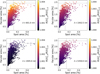 |
Fig. 2 Activity-induced apparent radius (as indicated by the colours) as a function of spot area coverage for selected wavelengths. The grey lines indicate the position of the maximum in the apparent radius for each of the wavelengths shown. We note that the average facular area is 1% and the mean spot area is 0.04%. An animated version of this figure is available online. |
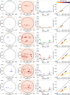 |
Fig. 3 Closer look at the different approaches presented in Fig. 1 by taking 6 days presented in Table 1, with their spot distribution in the first column and the faculae distribution in the second column, the apparent radius for approach 1 (black solid lines) and approach 2 (coloured solid lines) in column three, and scatterplots of the apparent radius as a function of wavelength (column four). We refer to the text for details of why those dates were chosen. |
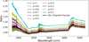 |
Fig. 4 Flux ratio between the faculae and the quiet Sun for the different approaches. Approach 1 (black line) is shown as black lines and the coloured lines indicate the flux rations for different μ positions. |
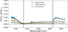 |
Fig. 6 Example of arbitrarily chosen spectra and fits to different wavelength regimes. The dashed black lines correspond to the fit given in Eq. (4), the dotted black line to Eq. (5), and the dash-dotted black line to Eq. (6). |
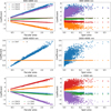 |
Fig. 7 Dependence of the fit coefficients for the different wavelength regimes from Eqs. (4)–(6) on the faculae and spot area coverage. The coefficients were multiplied by different factors as given in the legend in order to put them on equivalent scales. |
3.2 Impact on the transit depth and connection to JWST
We have discussed in the previous section the impact of the solar activity on the apparent radius. Lastly, we now want to consider the impact of the apparent solar radius on the transit depth of a planet itself. For this, we utilise Eq. (2) and the solar radius as calculate and presented in Fig. 1. We consider cases of two transiting planets: a Jupiter-sized and an Earth-sized one. The transit depth of a Jupiter-like planet around the Sun is 10 000 ppm, for the Earth it would be 100 ppm, solely based on the radii compared to the Sun. We also assume no chromatic effect of the planets (i.e. a planet without an atmosphere), we want to consider the impact of the solar apparent radius solely. The results of these calculations are presented in Fig. 8. Unsurprisingly, towards the visual part of the spectrum, the slope is positive and the transit depth lower. At around 16 000 nm, in approach 2, the planet radius is almost at the assumed 10 000 and 100 ppm level, respectively, as the apparent solar radius in the presence of solar activity is at a minimum (i.e. there is no change from the ‘quiet’, activity free solar radius). For approach 1 around 1600 nm, the transit becomes deeper due to the spots dominating the chromatic dependence. Rustamkulov et al. (2023) estimated the noise floor of JWST to be around 10 ppm. We now want to turn to at the amplitude of signal that the change in the level of the solar activity induces during the two transits considered. For this, we take the curves from Fig. 8 and calculate the minimum and maximum value of the transit depth for each wavelengths (i.e. the minimum and maximum activity induced contamination of the signal). We show the ratios of the minimum and maximum signal (i.e. the amplitude of the effect) in Fig. 9. The amplitude of the change in the solar level of activity is too small to be detected for an Earth-like transit (the values are below 10 ppm, however for a Jupiter-like transit in the ‘ground truth’ model (approach 2) the amplitude is high enough to be detected by JWST; hence, it presents a hurdle for the retrieval of a planetary atmosphere. We emphasise that this only means that the change in the amplitude of the apparent radius between low-and high solar activity cannot be measured by JWST; however, the transit depth of an Earth-like (as seen in Fig. 8) is above the noise floor.
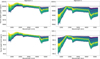 |
Fig. 8 Chromatic dependence of the transit depth for a Jupiter-like (top) and an Earth-like (bottom) planet. The dashed lines indicate the transit depth that is a result of the difference in radii with respect to the Sun (i.e. in the absence of both stellar activity and a planetary atmosphere). |
4 Summary and outlook
A planet’s transit depth depends, at first order, on the squares of the planet-to-star radius ratio. As stellar activity in the form of spots and faculae introduces a change in the apparent radius, it is crucial to understand the chromatic effect of the stellar variability to correct for it in atmospheric retrieval methods (Lim et al. 2023). We investigated two approaches to calculate the chromatic dependence of the apparent radius by using the Sun as a testbed, as it is the only star for which the active region distribution is well constrained. We found that calculating the apparent radius by the using simply the disc area coverage of a given feature and their disc integrated spectrum (i.e. as used by Seager & Shapiro 2024), generally underestimates the apparent radius compared to using the sophisticated approach that takes foreshortening effects and CLV into account. This underestimation would mean that the stellar contamination is not correctly removed in the transmission spectrum and, hence, the planetary radius end up overestimated. We parametrised the chromatic dependence of the apparent radius and have quantitatively shown that the faculae component is the important driver behind changes in the flux and that it is particularly important for wavelengths below 2000 nm. This is unsurprising as observations of both the Sun (for instance Chapman et al. 1997; Foukal 1998; Shapiro et al. 2016; Nèmec et al. 2022) and solar analogues (i.e. Lockwood et al. 2007; Radick et al. 2018, and references therein) show that the faculae contribution to stellar brightness variations is dominating over the spot contribution for low activity stars such as the Sun. We also present the fit coefficients for different activity levels for a Sun-like star as a recipe for mitigating stellar activity. We emphasise that the fitting coefficients presented are only applicable to stars with similar distributions in terms of the latitude of active regions (i.e. as depicted by the butterfly diagram) to the Sun.
Additionally, our results clearly show that on stars with similar activity to that of the Sun, un-occulted faculae will dominate the chromatic radius dependence of the star. In particular, if not taken into account properly in removing the stellar contamination in the transmission spectrum, the radius of the planet will be overestimated greatly. So far in the literature, cooler stars than the Sun have been targeted; hence, it is not straightforward to apply our findings to those stars. In particular, JWST mostly observes K- and M-type dwarfs, where the star-planet-ratio is larger (than e.g. for the Sun-Earth system). Recent developments in spectral modelling (i.e. Norris et al. 2023), indicate that faculae on M-dwarfs look very different than on the Sun; namely, their brightness contrast is negative. This puts certain claims reported in the literature for stars such as TRAPPIST-1 showing signs of un-occulted faculae (i.e Lim et al. 2023) under scrutiny. However, our results can be used for forward-modelling exercises for the upcoming Ariel mission Tinetti et al. (2022).
The primary implication of our results is that the negative slope in the transmission spectra in the visual wavelength regime, as reported in the literature, can be partially explained by un-occulted faculae. However, two things have to be kept in mind. Firstly, retrieval methods often do not account for CLV effects (e.g. Petit dit de la Roche et al. 2024; Radica et al. 2025). Secondly, faculae are approximated with a spectrum that is hotter than the stellar photosphere. As shown by Witzke et al. (2022), this is not even true for the Sun. In particular, a hotter stellar atmosphere would not be consistent with the observed limbbrightening by faculae, which can also be seen in simulations of faculae on other spectral types Norris et al. (2023). This highlights the particular importance of properly adopting faculae models in retrieval codes, as well as the need for better synergies between the exoplanet, stellar astrophysics and solar physics community.
We employed 1D models of both spots and faculae in the present work, where the limb darkening (or rather brightening) for the faculae was adjusted for in the solar case, in particular. Witzke et al. (2022) have shown that the 1D stellar atmosphere models that are regularly used to model the stellar contamination spectra do not agree with novel faculae models that are based on the 3D MDH Max Planck Institute for Solar System Research/University of Chicago Radiative Magnetohydrodynamics (MURaM, Vögler et al. 2004; Rempel 2014) simulations. In particular, the ‘3D’ faculae show an even stronger negative contrast around 1500 nm than predicted by the 1D models (Witzke et al. 2022). This once more highlights the need for physics-based models of stellar activity, especially for faculae. Qualitatively, for our results, that would mean that the slope in the visible wavelength regime is steeper. In addition, at around 1500 nm the apparent radius might reach values slightly below unity, as the faculae on the 3D simulations display a stronger negative contrast than their 1D counterparts.
Despite the limitations of current approaches commonly found in the literature, our results clearly show that for a star with the Sun, the change in the activity level cannot currently be detected by JWST if we consider an Earth-like planet, as the effect is below the noise floor for its instruments. However, in the case of a Jupiter-like transit, stellar activity contamination is easily detectable and therefore should be properly accounted for, especially in the case of un-occulted features.
The question of how to mitigate the stellar contamination if the magnetic field distribution is unknown, which is the case for any other star than the Sun, still remains. In particular, we have shown that the CLV plays a large role and that same distributions lead to the same results. The reality, however, is that even filling factors (i.e. area coverage) themselves are hard to constrain, and are treated as free parameters in forward models (i.e. Lim et al. 2023; Radica et al. 2025) to mitigate stellar activity in exoplanet atmosphere retrievals. As we have shown in the present work, there are degeneracies due do the exact distribution of the features, if the filling factors are very similar. The question still remains how we can estimate the filling factors. Mallonn et al. (2018); Rosich et al. (2020) have shown that it is possible to constrain filling factors and surface distributions better by utilising contemporaneous multi-technique (i.e. high-resolution spectroscopy combined with multi-colour photometry). In a follow-up work, we are planning to revisit such an approach and utilise available solar data (i.e. SSI – SORCE and HARPS-N spectral information) to investigate, with the Sun as ground truth once again, the potential of using stellar activity indicators to mitigate the stellar contamination in transmission spectroscopy.
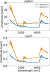 |
Fig. 9 Amplitude of the impact on the transit depth induced by solar activity (i.e. the difference between solar maximum and minimum. The dashed grey line on the top panel is the 10 ppm noise floor level for JWST as found by Rustamkulov et al. (2023). |
Data availability
Movie associated to Fig 2 is available at https://www.aanda.org
Acknowledgements
We thank the anonymous referee for their comments that helped improve the manuscript. This publication has been made possible by the Spanish grants PID2021-125627OB-C31 funded by MCIU/AEI/10.13039/501100011033 and by “ERDF A way of making Europe”, PID2020-120375GB-I00 funded by MCIU/AEI, by the programme Unidad de Excelencia María de Maeztu CEX2020-001058-M, by the Generalitat de Catalunya/CERCA programme, by the SGR 01526/2021, the European Research Council (ERC) under the European Union’s Horizon Europe programme (ERC Advanced Grant SPOTLESS; no. 101140786, ERC Synergy Grant REVEaL grant no. 101118581) and the Marie Skłodowska-Curie Actions grant agreement no. 101149286 (INCITE).
References
- Ahrer, E.-M., Radica, M., Piaulet-Ghorayeb, C., et al. 2025, ApJ, 985, L10 [Google Scholar]
- Ardévol Martínez, F., Min, M., Kamp, I., & Palmer, P. I., 2022, A&A, 662, A108 [NASA ADS] [CrossRef] [EDP Sciences] [Google Scholar]
- Ball, W. T., Unruh, Y. C., Krivova, N. A., et al. 2012, A&A, 541, A27 [NASA ADS] [CrossRef] [EDP Sciences] [Google Scholar]
- Böker, T., Arribas, S., Lützgendorf, N., et al. 2022, A&A, 661, A82 [NASA ADS] [CrossRef] [EDP Sciences] [Google Scholar]
- Brandt, P. N., Schmidt, W., & Steinegger, M., 1990, Sol. Phys., 129, 191 [Google Scholar]
- Castelli, F., & Kurucz, R. L., 1994, A&A, 281, 817 [NASA ADS] [Google Scholar]
- Chapman, G. A., Cookson, A. M., & Dobias, J. J., 1997, ApJ, 482, 541 [CrossRef] [Google Scholar]
- Charbonneau, D., Brown, T. M., Noyes, R. W., & Gilliland, R. L., 2002, ApJ, 568, 377 [Google Scholar]
- Ermolli, I., Matthes, K., Dudok de Wit, T., et al. 2013, Atmos. Chem. Phys., 13, 3945 [NASA ADS] [CrossRef] [Google Scholar]
- Fligge, M., Solanki, S. K., & Unruh, Y. C., 2000, A&A, 353, 380 [NASA ADS] [Google Scholar]
- Foukal, P., 1998, ApJ, 500, 958 [NASA ADS] [CrossRef] [Google Scholar]
- Fournier-Tondreau, M., Pan, Y., Morel, K., et al. 2025, MNRAS, 539, 422 [Google Scholar]
- Jakobsen, P., Ferruit, P., Alves de Oliveira, C., et al. 2022, A&A, 661, A80 [NASA ADS] [CrossRef] [EDP Sciences] [Google Scholar]
- Kopp, G., Nèmec, N.-E., & Shapiro, A. 2024, ApJ, 964, 60 [Google Scholar]
- Krivova, N. A., Solanki, S. K., Fligge, M., & Unruh, Y. C., 2003, A&A, 399, L1 [NASA ADS] [CrossRef] [EDP Sciences] [Google Scholar]
- Kurucz, R. L., 1992, Rev. Mex. Astron. Astrofis., 23, 45 [Google Scholar]
- Lim, O., Benneke, B., Doyon, R., et al. 2023, ApJ, 955, L22 [NASA ADS] [CrossRef] [Google Scholar]
- Lockwood, G. W., Skiff, B. A., Henry, G. W., et al. 2007, ApJS, 171, 260 [Google Scholar]
- Lueber, A., Novais, A., Fisher, C., & Heng, K., 2024, A&A, 687, A110 [NASA ADS] [CrossRef] [EDP Sciences] [Google Scholar]
- Mallonn, M., Herrero, E., Juvan, I. G., et al. 2018, A&A, 614, A35 [NASA ADS] [CrossRef] [EDP Sciences] [Google Scholar]
- Matchev, K. T., Matcheva, K., & Roman, A., 2022, ApJ, 930, 33 [NASA ADS] [CrossRef] [Google Scholar]
- Mayor, M., & Queloz, D., 1995, Nature, 378, 355 [Google Scholar]
- Nèmec, N. E., Shapiro, A. I., Işık, E., et al. 2022, ApJ, 934, L23 [CrossRef] [Google Scholar]
- Norris, C. M., Unruh, Y. C., Witzke, V., et al. 2023, MNRAS, 524, 1139 [NASA ADS] [CrossRef] [Google Scholar]
- Petit dit de la Roche, D. J. M., Chakraborty, H., Lendl, M., et al. 2024, A&A, 692, A83 [NASA ADS] [CrossRef] [EDP Sciences] [Google Scholar]
- Rackham, B. V., Apai, D., & Giampapa, M. S., 2019, AJ, 157, 96 [Google Scholar]
- Rackham, B. V., Espinoza, N., Berdyugina, S. V., et al. 2023, RAS Tech. Instrum., 2, 148 [NASA ADS] [CrossRef] [Google Scholar]
- Radica, M., Piaulet-Ghorayeb, C., Taylor, J., et al. 2025, ApJ, 979, L5 [NASA ADS] [CrossRef] [Google Scholar]
- Radick, R. R., Lockwood, G. W., Henry, G. W., Hall, J. C., & Pevtsov, A. A., 2018, ApJ, 855, 75 [Google Scholar]
- Rempel, M., 2014, ApJ, 789, 132 [Google Scholar]
- Rosich, A., Herrero, E., Mallonn, M., et al. 2020, A&A, 641, A82 [NASA ADS] [CrossRef] [EDP Sciences] [Google Scholar]
- Rustamkulov, Z., Sing, D. K., Mukherjee, S., et al. 2023, Nature, 614, 659 [NASA ADS] [CrossRef] [Google Scholar]
- Schou, J., Scherrer, P. H., Bush, R. I., et al. 2012, Sol. Phys., 275, 229 [Google Scholar]
- Seager, S., & Sasselov, D. D., 2000, ApJ, 537, 916 [Google Scholar]
- Seager, S., & Shapiro, A. I., 2024, ApJ, 970, 155 [Google Scholar]
- Shapiro, A. I., Solanki, S. K., Krivova, N. A., Yeo, K. L., & Schmutz, W. K., 2016, A&A, 589, A46 [NASA ADS] [CrossRef] [EDP Sciences] [Google Scholar]
- Shapiro, A. I., Solanki, S. K., Krivova, N. A., et al. 2017, Nat. Astron., 1, 612 [NASA ADS] [CrossRef] [Google Scholar]
- Solanki, S. K., Krivova, N. A., & Haigh, J. D., 2013, ARA&A, 51, 311 [Google Scholar]
- Tinetti, G., Vidal-Madjar, A., Liang, M.-C., et al. 2007, Nature, 448, 169 [NASA ADS] [CrossRef] [Google Scholar]
- Tinetti, G., Eccleston, P., Lueftinger, T., et al. 2022, in European Planetary Science Congress, EPSC2022–1114 [Google Scholar]
- Unruh, Y. C., Solanki, S. K., & Fligge, M., 1999, A&A, 345, 635 [NASA ADS] [Google Scholar]
- Vögler, A., Bruls, J. H. M. J., & Schüssler, M., 2004, A&A, 421, 741 [NASA ADS] [CrossRef] [EDP Sciences] [Google Scholar]
- Witzke, V., Shapiro, A. I., Kostogryz, N. M., et al. 2022, ApJ, 941, L35 [NASA ADS] [CrossRef] [Google Scholar]
- Yan, F., Casasayas-Barris, N., Molaverdikhani, K., et al. 2019, A&A, 632, A69 [NASA ADS] [CrossRef] [EDP Sciences] [Google Scholar]
- Yeo, K. L., Krivova, N. A., Solanki, S. K., & Glassmeier, K. H., 2014, A&A, 570, A85 [NASA ADS] [CrossRef] [EDP Sciences] [Google Scholar]
All Tables
All Figures
|
Fig. 1 Dependence of the apparent solar radius as a function of solar activity for the different approaches. Top: spot area coverage as a function of the time for solar cycle 24. The spot disc area coverage is shown in different colours. Bottom: approach 1 corresponds to the disc integrated spectra and approach 2 takes the spectra of each pixel of the HMI maps into account. |
| In the text | |
|
Fig. 2 Activity-induced apparent radius (as indicated by the colours) as a function of spot area coverage for selected wavelengths. The grey lines indicate the position of the maximum in the apparent radius for each of the wavelengths shown. We note that the average facular area is 1% and the mean spot area is 0.04%. An animated version of this figure is available online. |
| In the text | |
|
Fig. 3 Closer look at the different approaches presented in Fig. 1 by taking 6 days presented in Table 1, with their spot distribution in the first column and the faculae distribution in the second column, the apparent radius for approach 1 (black solid lines) and approach 2 (coloured solid lines) in column three, and scatterplots of the apparent radius as a function of wavelength (column four). We refer to the text for details of why those dates were chosen. |
| In the text | |
|
Fig. 4 Flux ratio between the faculae and the quiet Sun for the different approaches. Approach 1 (black line) is shown as black lines and the coloured lines indicate the flux rations for different μ positions. |
| In the text | |
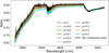 |
Fig. 5 Similar to Fig. 4, but for spots. |
| In the text | |
|
Fig. 6 Example of arbitrarily chosen spectra and fits to different wavelength regimes. The dashed black lines correspond to the fit given in Eq. (4), the dotted black line to Eq. (5), and the dash-dotted black line to Eq. (6). |
| In the text | |
|
Fig. 7 Dependence of the fit coefficients for the different wavelength regimes from Eqs. (4)–(6) on the faculae and spot area coverage. The coefficients were multiplied by different factors as given in the legend in order to put them on equivalent scales. |
| In the text | |
|
Fig. 8 Chromatic dependence of the transit depth for a Jupiter-like (top) and an Earth-like (bottom) planet. The dashed lines indicate the transit depth that is a result of the difference in radii with respect to the Sun (i.e. in the absence of both stellar activity and a planetary atmosphere). |
| In the text | |
|
Fig. 9 Amplitude of the impact on the transit depth induced by solar activity (i.e. the difference between solar maximum and minimum. The dashed grey line on the top panel is the 10 ppm noise floor level for JWST as found by Rustamkulov et al. (2023). |
| In the text | |
Current usage metrics show cumulative count of Article Views (full-text article views including HTML views, PDF and ePub downloads, according to the available data) and Abstracts Views on Vision4Press platform.
Data correspond to usage on the plateform after 2015. The current usage metrics is available 48-96 hours after online publication and is updated daily on week days.
Initial download of the metrics may take a while.