| Issue |
A&A
Volume 705, January 2026
|
|
|---|---|---|
| Article Number | A180 | |
| Number of page(s) | 16 | |
| Section | Extragalactic astronomy | |
| DOI | https://doi.org/10.1051/0004-6361/202557349 | |
| Published online | 21 January 2026 | |
Kinematic scaling relations of disc galaxies from ionised gas at z ∼ 1 and their connection with dark matter haloes
1
Leiden Observatory, Leiden University P.O. Box 9513 2300 RA Leiden, The Netherlands
2
Dipartimento di Fisica e Astronomia, Università degli Studi di Firenze via G. Sansone 1 50019 Sesto Fiorentino Firenze, Italy
3
Department of Physics and Astronomy, Johns Hopkins University 3400 N. Charles Street Baltimore MD 21218, USA
4
INAF – Padova Astronomical Observatory Vicolo dell’Osservatorio 5 I-35122 Padova, Italy
5
Sterrenkundig Observatorium, Universiteit Gent Krijgslaan 281 S9 9000 Gent, Belgium
★ Corresponding author: This email address is being protected from spambots. You need JavaScript enabled to view it.
Received:
22
September
2025
Accepted:
30
November
2025
Abstract
We derive the Tully-Fisher (TFR; M* − Vcirc, f) and Fall (FR; j* − M*) relations at redshift z = 0.9 using a sample of 43 main-sequence disc galaxies with Hα IFU data and JWST/HST imaging. The strength of our analysis lies in the use of state-of-the-art 3D kinematic models to infer galaxy rotation curves, the inclusion of near-IR bands and their morphological modelling, and the application of homogeneous spectral energy distribution modelling to our photometry measurements to estimate stellar masses. After correcting the inferred Hα velocities for asymmetric drift, we find a TFR of the form log(M*/M⊙) = a log(Vcirc,f/ 150 km s−1 + b, with a = 3.82−0.40+0.55 and b = 10.27−0.07+0.06, as well as a FR of the form log(j*/kpc km s−1) = alog(M*/1010.5 M⊙)+b, with a = 0.44−0.06+0.06 and b = 2.86−0.02+0.02. Compared with their z = 0 counterparts, we found moderate evolution in the TFR and strong evolution in the FR over the past 8 Gyr. We interpreted our findings in the context of the galaxy-to-halo scaling parameters fM = M*/Mvir and fj = j*/jvir. We inferred that fj shows little redshift evolution and depends very weakly on M*, with typical values around fj ∼ 0.8. As for fM, we find it to be higher and less dependent on M* at z = 0.9 than at z = 0. We discuss how interpreting our observed fM − M* relations within the cold dark matter framework implies necessarily that the galaxy populations at z = 0.9 and z = 0 are not the progenitor nor descendant of one another. The alternative scenario is that the z = 0.9 scaling relations are incorrect due to strong selection effects, unidentified systematics, or the possibility that Hα kinematics may not be a reliable dynamical tracer. Such problems would affect not only our work but also previous studies on the same subject.
Key words: galaxies: evolution / galaxies: formation / galaxies: fundamental parameters / galaxies: high-redshift / galaxies: kinematics and dynamics
© The Authors 2026
 Open Access article, published by EDP Sciences, under the terms of the Creative Commons Attribution License (https://creativecommons.org/licenses/by/4.0), which permits unrestricted use, distribution, and reproduction in any medium, provided the original work is properly cited.
This article is published in open access under the Subscribe to Open model. This email address is being protected from spambots. You need JavaScript enabled to view it. to support open access publication.
1. Introduction
Two of the most fundamental scaling relations for disc galaxies are those connecting their stellar mass (M*) with their rotational velocities (V) and their stellar specific angular momentum (j*), i.e. the stellar Tully-Fisher (TFR; Tully & Fisher 1977; Bell & de Jong 2001) and Fall (FR; Fall 1983) relations. These scaling relations are closely intertwined with the process of galaxy evolution. According to our current galaxy formation theories, dark matter and baryons acquire their angular momentum through tidal torques from neighbouring systems before virialisation. Upon the dissipation and gravitational collapse of the baryons, the global angular momentum is approximately conserved, leading the baryons in disc galaxies to settle into relatively thin disc-like structures supported by rotation and embedded in more extended dark matter haloes without significant rotational support (e.g. Peebles 1969; Binney 1977; White & Rees 1978; Fall & Efstathiou 1980; Blumenthal et al. 1984; White 1984; Dalcanton et al. 1997; Mo et al. 1998). In this way, the distribution of angular momentum is thought to set the rotational velocity and mass distribution of galaxies, regulating also their morphology and gas content (e.g. Romanowsky & Fall 2012; Obreschkow & Glazebrook 2014; Cortese et al. 2016; Lagos et al. 2017; Swinbank et al. 2017; Sweet et al. 2020; Mancera Piña et al. 2021b; Geesink et al. 2025). Observational constraints on the TFR and FR provide crucial benchmarks for galaxy formation models.
In the nearby Universe, at z ∼ 0, the TFR and FR have been studied in detail and found to be well described by unbroken power laws of the form M* ∝ Va and j* ∝ M*a, respectively. These slopes are found to be a ≈ 3.5 − 5 for the TFR (e.g. Bell & de Jong 2001; Reyes et al. 2011; Ponomareva et al. 2017; Catinella et al. 2023; Marasco et al. 2025) and a ≈ 0.5 − 0.6 for the FR (e.g. Posti et al. 2018; Mancera Piña et al. 2021a; Hardwick et al. 2022; Di Teodoro et al. 2021, 2023; Marasco et al. 2025). At higher redshifts, the situation remains significantly less certain. Although different works have studied the TFR and FR up to z ∼ 2.5 (e.g. Conselice et al. 2005; Cresci et al. 2009; Burkert et al. 2016; Contini et al. 2016; Di Teodoro et al. 2016; Price et al. 2016; Harrison et al. 2017; Swinbank et al. 2017; Gillman et al. 2019; Marasco et al. 2019; Sweet et al. 2019; Pelliccia et al. 2019; Tiley et al. 2019; Mercier et al. 2023), there is no consensus on whether or not the relations (slopes, intercept, intrinsic scatter) evolve with z (see Übler et al. 2017; Pelliccia et al. 2019; Bouché et al. 2021; Sharma et al. 2024; Espejo Salcedo et al. 2025). Some of the difficulty in tracing the evolution of the TFR and FR arises from observational uncertainties and methodological limitations when studying high-z disc galaxies (e.g. Rizzo et al. 2022; Araujo-Carvalho et al. 2025; Sharma et al. 2025). Two major concerns in most previous works are the derivation of galaxy kinematics and of stellar masses. Obtaining reliable kinematics at high z is challenging, due to both the limited quality of the data (low spatial resolution, low signal-to-noise ratio, short radial extent) and the intrinsically complex structure of young galaxies. In addition, M* is typically estimated through spectral energy distribution (SED) fitting (or by adopting a fixed mass-to-light ratio), often relying on photometry of variable quality and lacking rest-frame near-infrared (NIR) coverage, which is crucial for constraining the underlying stellar mass distribution.
In this work, we revisit the evolution of the TFR and FR at z ∼ 1 while addressing these limitations. In particular, our study improves upon previous efforts in several key ways: (i) We use well-tested software that takes into account observational effects for data of limited quality in a self-consistent way. (ii) We exploit new JWST observations providing exquisite NIR data, improving the stellar mass density profiles. (iii) We apply asymmetric drift corrections to take into account the pressure-supported motions of ionised gas and stars compared to cold gas (which is typically used at z = 0); this is crucial as it is a systematic effect that depends on M*. (iv) Rather than assuming stellar-to-halo mass and specific angular momentum ratios that depend on abundance-matching calibrations, we show that these can be directly derived from the observed TFR and FR. (v) Finally, we assess the evolution of the TFR and FR at z ∼ 1 by contrasting against new and improved z = 0 determinations (Marasco et al. 2025). Throughout this work, we adopt a Λ cold dark matter (ΛCDM) cosmology with Ωm, 0 = 0.3, ΩΛ, 0 = 0.7, and H0 = 70 km s−1 Mpc−1.
2. Data and sample selection
For this study, we made use of data tracing the resolved stellar mass distribution and kinematics of galaxies at z ≈ 1. For the kinematics, we relied on the integral field unit (IFU) spectroscopy from the KROSS (Stott et al. 2016) and KMOS3D (Wisnioski et al. 2015) surveys. These surveys mapped the Hα distribution and kinematics of galaxies at z ∼ 0.6 − 2.5 using the KMOS instrument at the VLT. The spectral resolution of the data is R = λ/Δλ ∼ 3500 − 4000, which for Hα at our z corresponds to σ ∼ 40 km/s. The typical full width at half maximum (FWHM) of the point-spread function (PSF) is ∼0.5 − 0.8 arcsec (Stott et al. 2016; Wisnioski et al. 2019). We note that the kinematics of these samples have been studied before (e.g., Stott et al. 2016; Burkert et al. 2016; Harrison et al. 2017; Übler et al. 2017; Tiley et al. 2019; Sharma et al. 2021), although with approaches different from ours, as discussed below.
For this work, we required a galaxy sample that met several selection criteria on the kinematic data. We started by visually inspecting all the position-velocity (PV) slices along the major and minor axes of the galaxies in the parent sample, keeping only those systems with a high signal-to-noise (S/N) and compelling regular kinematics (i.e. clear velocity gradients in the major-axis PV, no gradients in the minor-axis PV, no signs of mergers) to ensure a clean sample of rotating discs. Next, we selected against poorly resolved galaxies with Hα emission less extended than ∼2 times the PSF. As shown below, we verified that this criterion does not appear to significantly bias the optical mass-size relation of our galaxies, which is consistent with literature relations for the star-forming disc population.
In addition, we require that the galaxies have available HST- or JWST-based morphological Sérsic models. Specifically, we rely on the results from van der Wel et al. (2012), Martorano et al. (2024), and Martorano et al. (2026), who carefully built PSFs and used GALFIT (Peng et al. 2010, see Martorano et al. 2023 for the treatment of the uncertainties) to obtain accurate effective radii (Reff, *), Sérsic indices (n), position angles, and axial ratios (b/a). We prioritised the parameters obtained from the reddest available band, which is f444w from NIRCam on JWST for 60% of our final sample (see below) and f160w from WFC3 on HST for the remaining 40%. These parameters and our M* estimates (described next) define Σ*(R), our stellar-mass surface-density profiles. We note that at our redshifts, f160w and f444w trace rest-frame emission at 0.81 μm and 2.33 μm, respectively, roughly corresponding to the rest-frame I- and K-bands. At our redshift and M* range, galaxy sizes in these bands agree within 10–20% (van der Wel et al. 2014; Suess et al. 2022).
A key aspect of this study is the use of robust M* estimates, which we obtained using the SED fitting approach by Marasco et al. (2025) and exploiting our HST (ACS or WFC3) and/or JWST (NIRCam) photometry. In particular, we used the publicly available images from the following surveys: CANDELS (Grogin et al. 2011; Koekemoer et al. 2011), COSMOS (Koekemoer et al. 2007; Scoville et al. 2007), PRIMER (Dunlop et al. 2021), JADES (Eisenstein et al. 2023), and COSMOS-Web (Casey et al. 2023). These surveys provide imaging in (some of) the following filters: f444w, f356w, f277w, f150w, f115w, and f090w from JWST, and f160w, f125w, f105w, f814w, f850lp, and f606w from HST. Using only space-based imaging (a condition not always imposed in previous studies) is crucial, as it has significantly better spatial resolution, photometric calibration, and overall image quality than ground-based data. Moreover, unlike previous studies, we used JWST rest-frame bands, enabling us to better characterise the stellar masses of our sample. We carefully extracted the photometry (see Marasco et al. 2025 for full details) in the available bands and modelled the SED with the software BAGPIPES (Carnall et al. 2018). We adopted ‘non-parametric’ star-formation histories, considering the stellar population models from Bruzual & Charlot (2003, 2016 version)1, the dust model from Charlot & Fall (2000), and a Kroupa (2002) initial mass function. The redshift is fixed to the Hα value from the KROSS and KMOS3D surveys. We only considered galaxies with fluxes in at least four bands (we typically have five or six bands but as many as ten) and whose model SEDs provide a high-quality fit to the data (p(> χ2) > 0.05; see Marasco et al. 2025). Marasco et al. (2025) showed that their SED-based and dynamical M* estimates in local disc galaxies (e.g. Posti et al. 2019a; Schombert et al. 2022; Mancera Piña et al. 2025) agree within ∼0.2 dex across nearly six orders of magnitude in M*, which implies that they can be used interchangeably in the study of scaling relations and their evolution.
Assuming an intrinsic disc axial ratio q0 = 0.2 (e.g. Fouque et al. 1990), we derived galaxy inclinations from the observed b/a using the standard (Hubble 1926) relation cos2(i) = ((b/a)2 − q02)/(1 − q02). We excluded galaxies with i < 30° (where small errors in i cause significant velocity uncertainties) and i > 80° (for which ring-by-ring kinematic models are not well suited due to the overlap of different lines of sight). From the remaining sample, we retained only systems for which 3D kinematics can be reliably modelled. For this, we used the forward modelling software 3DBarolo (Di Teodoro & Fraternali 2015), which accounts for beam smearing and enables robust recovery of intrinsic rotation curves and velocity dispersions. Full details of the kinematic modelling are provided in Appendix A.
After applying our selection criteria, we selected 43 disc galaxies. Our sample spans the range 0.78 < z < 1.03 with a median z of 0.89. This redshift range corresponds to cosmic ages between 6.7 Gyr and 5.6 Gyr. The galaxies have stellar masses in the range 5 × 10⁹ < M*/M⊙ < 2 × 10¹¹. Given all our selection cuts based on data quality, establishing a selection function is far from straightforward. However, we found that our final sample is representative of the typical star-forming galaxy population, characterised by regular kinematics. This is illustrated in Fig. 1, showing that the sample follows the star formation main sequence (SFMS, top left panel) at z ≈ 0.9, is dominated by rotation2 (top right panel), has a Sérsic index distribution typical of discs (median n ≈ 1.3, bottom left panel), and follows the M* − Reff, * relation from Martorano et al. (2024) at z = 0.9 and van der Wel et al. (2014) at z = 0.75 (bottom right panel3). Table D.1 lists the main properties of our sample.
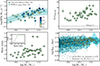 |
Fig. 1. Top left: The SFMS defined by our high-z galaxies, colour-coded by their redshift. The reference SFMS from Leja et al. (2022) is shown. Star formation rates come from our SED fitting. Top right: Rotation to dispersion ratio for our galaxy sample. Bottom left: Sérsic index as a function of M*. The inset shows the cumulative distribution of the Sérsic indices. Bottom right: Stellar mass-size relation. Our galaxies (green markers) are contrasted against (1) the individual measurements from Martorano et al. (2024) at 0.8 ≤ z ≤ 1 (blue markers) and their 1 and 2 σ ranges (blue bands), and (2) the relation from van der Wel et al. (2014) at z = 0.75 after applying approximate corrections to account for the sizes differences in optical vs. NIR bands. |
3. Estimating Vcirc, f and j*
Our kinematic modelling described in Appendix A allows us to obtain the intrinsic rotational velocity of the ionised gas (VHα(R)) and its velocity dispersion (σHα(R)). Instead, the TFR requires the circular speed (Vcirc4), and the FR requires the stellar rotational velocities (V*). If derived from cold gas (e.g. H I or CO), the rotational velocities could be used directly to build the TFR and FR, since the cold gas has a high rotational support and low pressure-supported motions, and the rotational speeds are close to both Vcirc and V* (at least for M* ≳ 5 × 10⁸ M⊙, see Mancera Piña et al. 2021a). However, for ionised gas at z ∼ 1 (see also Catinella et al. 2023 at z = 0), the velocity dispersions tend to be higher and the rotation-to-dispersion ratios lower, making it imperative to correct for the different asymmetric drift of the stars and ionised gas. In particular, Vcirc, V*, and our measured VHα are related through the expressions
 (1)
(1)
 (2)
(2)
where VAD, * and VAD, Hα are the asymmetric drift (AD) corrections to account for the pressure support provided by the stars and the ionised gas, respectively. Therefore, the steps to follow are first to convert our VHα into Vcirc, and then Vcirc into V*. We note that in this study, all uncertainties are propagated throughout our calculations using Monte Carlo sampling (with measurement errors assumed to be Gaussian). The quoted errors correspond to the difference between the 84th and 16th percentiles and are propagated using the full sampling of the posterior distributions.
Under the assumptions of constant scale heights and relatively thin discs, the AD corrections (Binney & Tremaine 2008) take the approximate form
 (3)
(3)
with Σ the ionised gas or stellar surface density, and β ≡ σz/σR, with σz and σR the vertical and radial components of the stellar or ionised gas velocity dispersion profiles.
We start by computing VAD, Hα. For this, we make the common assumption that the gas velocity dispersion is isotropic, which sets β = 1. Next we assume a constant σz, Hα(R), given by the median value of our observed σHα5. Regarding the surface density, although in principle we have access to ΣHα, the Hα data’s spatial resolution is too low to infer detailed radial profiles. Instead, we assume that Hα shares the same Sérsic index as the stellar disc, but with Reff, Hα = 1.13(±0.05) Reff, *, as found for disc galaxies within our M* and z range (Nelson et al. 2016; Wilman et al. 2020). With this VAD, Hα, we can convert VHα into Vcirc.
Kinematic data at z ∼ 0 have extended H I data that can be traced far out the disc with many resolution elements to measure the characteristic flat velocity of Vcirc(R) (Vcirc, f), which we need for the TFR. In contrast, high-z rotation curves have more limited resolution (typically three to five (nearly) independent resolution elements, see Appendix A) and do not extend as much as H I, which prevents us from performing the same measurement. Instead, we implement the following approach. We first fit Vcirc(R) with the arctan rotation curve model from Courteau et al. (2007), i.e. Vcirc(R) = (2/π) Va arctan(R/rt), with Va the asymptotic velocity of the rotation curve and rt a turnover radius between the rising and outer part of the rotation curve. In practice, the fit is done using the Bayesian Nested Sampling software dynesty (Speagle 2020), minimising a χ2 likelihood. From empirical tests using a sample of z = 0 disc galaxies with high-resolution kinematics (described in Appendix B), we find that we can estimate Vcirc, f with a ∼1% accuracy, by evaluating the best-fit arctan model at R = 2 Reff, * for galaxies with Va ≥ 100 km/s, (as those in our high-z sample), and at R = 3 Reff, * for lower Va. From this, we obtain the Vcirc, f needed for the TFR.
Next, we focus on VAD, *, which allows us to estimate V* for the FR. We follow the procedure detailed in Mancera Piña et al. (2021a). Specifically, as supported by theoretical and observational work at z = 0 (van der Kruit 1988; Martinsson et al. 2013), we consider that the stellar velocity dispersion profile has a radial profile of the form
![Mathematical equation: $$ \begin{aligned} \sigma _{z,*}(R)/\mathrm {km\,s}^{-1} = \mathrm{max} [\sigma _{z_{0,*}}\exp (-R/1.19R_{\rm eff,*}),\ 10], \end{aligned} $$](/articles/aa/full_html/2026/01/aa57349-25/aa57349-25-eq8.gif) (4)
(4)
with an empirical σz0, * derived by Mancera Piña et al. (2021a) based on measurements of disc galaxies at z = 0 (see also e.g. Martinsson et al. 2013) given by
 (5)
(5)
which we assume not to evolve with z. The above calibrations are semi-empirical, but it is worth noting that detailed measurements show some degree of diversity among galaxies (Mogotsi & Romeo 2019). Finally, we consider β = 0.8 ± 0.2, consistent with the values found for nearby disc galaxies by Mogotsi & Romeo (2019). With all of the above, we compute VAD, * and convert Vcirc into V*.
With V*, we can determine j*, which is defined as
 (6)
(6)
For z = 0 data, Eq. (6) is computed by summing the high-resolution rotation curves and mass profiles (e.g. Posti et al. 2018; Mancera Piña et al. 2021a; Di Teodoro et al. 2023). For the z = 0.9 data, we rely on our Sérsic models for Σ* and on new arctan fits for V*(R). We integrate Eq. (6) (using deprojected parameters, considering the inclination angle) up to Rout = 10 Reff, ensuring the convergence of j*. As detailed in Appendix B, we have tested our procedure on a comparison sample at z = 0, finding that j* is recovered with a ∼5% accuracy.
Before delving into the best-fitting TFR and FR implied by our measurements, we emphasise the importance of applying AD corrections when analysing ionised gas kinematics, which is often overlooked in studies of the TFR and FR at high-z. As mentioned before, using such corrections is key to account for the varying rotation-to-dispersion ratios arising from various kinematic tracers at different redshifts, which are also a function of M* since typically low-mass galaxies have less rotational support (Fig. 1). To illustrate this, we quote the average differences in log(Vcirc, f) and log(j*) for our galaxy sample implementing or not the AD corrections. At log(M*/M⊙) = 10, 10.5, and 11, the AD-corrected values for log(Vcirc, f) are typically higher by about 0.09 dex, 0.04 dex, and 0.02 dex, respectively. Similarly, at the same masses, the AD-corrected values for log(j*) are higher by about 0.05 dex, 0.02 dex, and 0.0 dex, on average. As we discuss in the next section, these offsets are large enough to impact the best-fitting TFR and FR.
4. Scaling relations
4.1. Scaling laws at z = 0.9
In Fig. 2, we show our measurements in the M* − Vcirc, f and j* − M* planes. As found at low-z, our high-z galaxies follow well-defined sequences of increasing Vcirc, f and j* with increasing M*. In Fig. A.3, we show that at fixed M* galaxies with a high Vf/σmed also have a high Vcirc, f and j*. We parametrise the observed distributions in the M* − Vcirc, f and j* − M* planes with power-law models of the form
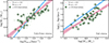 |
Fig. 2. Our z = 0.9 scaling laws. The TFR is shown on the left, and the FR on the right. Our measurements are shown with the green markers, while the best-fit relations and their 1σ confidence bands are shown as solid pink curves and bands, respectively. For comparison, we show the z = 0 TFR and FR from Marasco et al. (2025). |
 (7)
(7)
 (8)
(8)
where a is the slope of the relation and b is the intercept at our pivot mass and velocity. The pivot values of 1010.5 M⊙ and 150 km/s, chosen to be relatively close to the median values for our high-z sample, help in reducing the covariance between slopes and intercepts. In practice, the power-law fits to our TFR and FR are obtained using dynesty, adding an extra term to allow for intrinsic scatter perpendicular to the best-fit relation (ϵ⊥, the scatter unaccounted for by the observational uncertainties and therefore assumed to be intrinsic to the relations), and including uncertainties in both variables. We use flat priors for a, and b, and ϵ⊥ ≥ 0 for ϵ⊥. The best-fitting relations are shown in Fig. 2, and the best-fitting coefficients are listed in Table 1, where we also quote the observed vertical RMS scatter of the relations (σM* and σj*). We emphasise that σM* and σj* measure the scatter of the data, but do not weight the observational errors, while ϵ⊥ does, and it is assumed to be inherent to the scaling laws.
Best-fitting parameters (α, β, ϵ⊥) and vertical RMS scatter (σM* for the TFR and σj* for the FR) of our z = 0.9 TFR and FR.
The literature on the TFR and FR at z ∼ 1 is extensive, as recently summarised in Sharma et al. (2024) and Espejo Salcedo et al. (2025). Formally, the slope of our TFR is higher than the value of a = 3.03 by Sharma et al. (2024) and similar to those (a ∼ 3.6 − 3.8) reported by Di Teodoro et al. (2016), Harrison et al. (2017), Übler et al. (2017), Pelliccia et al. (2019), Tiley et al. (2019), Abril-Melgarejo et al. (2021), although it should be kept in mind the usage of different velocity conventions when defining the TFR, as well as the fact that some of the above studies fixed the slope to the local value from Reyes et al. (2011). Our FR slope is slightly below the a ∼ 0.5 − 0.6 reported by Harrison et al. (2017), Gillman et al. (2020) and Bouché et al. (2021), but entirely consistent within the uncertainties. Comparing the intercepts is more challenging because different studies use different pivot points; however, a visual inspection suggests fair agreement within ∼10 − 20%. The level of agreement among the various studies is encouraging, though somewhat surprising given the differing analyses. Given our thorough methodology (kinematic modelling and beam smearing corrections are more robustly determined, NIR JWST data are considered for SED fitting and surface brightness profiles, and realistic AD corrections are incorporated), we expect our best-fitting parameters to be as accurate as possible, considering the quality of the currently available data.
4.2. Evolution since the Universe’s half-age
Here we explore whether the scaling relations have evolved since z ∼ 1. Among the many low-z measurements, we adopt Marasco et al. (2025) as our z = 0 reference for three main reasons: (1) their analysis is based on the SPARC sample (Lelli et al. 2016), which we used to calibrate our methods (Appendix B); (2) their M* estimates are based on the same technique as ours; and (3) they adopt the same pivot values in their fitting (1010.5 M⊙ and 150 km/s), which simplifies the comparison. We note that Marasco et al. (2025) used directly H I kinematics to estimate Vcirc, f and j* without applying AD corrections, but we do not expect this to introduce big differences since rotation-to-dispersion ratios of H I data in the nearby Universe are much larger than those of our sample, leading to small differences between VH I, Vcirc, f, and V*, especially at M* > 108 M⊙ (Mancera Piña et al. 2021a). Marasco et al. (2025) reports a slope a = 5.21 ± 0.18, intercept b = 10.16 ± 0.03, intrinsic scatter ϵ⊥ = 0.039, and vertical observed scatter σM* = 0.274 for the local TFR, and a = 0.52 ± 0.03, b = 3.04 ± 0.03, ϵ⊥ = 0.128, and σj* = 0.171 for the local FR (similar to e.g. Posti et al. 2018; Mancera Piña et al. 2021a).
As shown in Fig. 2, our TFR and FR at z = 0.9 differ from those at z = 0. The evolution of the relations can also be visualised in Fig. 3, where we compare the posterior distributions of our best-fitting parameters to those of Marasco et al. (2025). As seen from Fig. 3 (note that unaccounted uncertainties in masses and kinematics may further broaden the confidence levels), our results present moderate evidence of the evolution of the TFR, and strong evidence of the evolution of the FR. In both relations, the evolution is driven by changes in slopes and intercepts, rather than by the intrinsic scatter. Near z ∼ 1, the TFR is shallower and has a higher intercept by about 0.1 dex. On the other hand, the FR has a slightly shallower slope (unlike the substantial changes reported by Espejo Salcedo et al. 2025 at z ≈ 1.5 − 2.5) and its intercept is lower by ∼0.2 dex. This latter offset has also been found by theoretical studies based on disc-stability conditions (Obreschkow et al. 2015) and semi-analytical models (Stevens et al. 2016), as well as observational studies (Harrison et al. 2017; Swinbank et al. 2017).
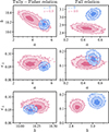 |
Fig. 3. Posterior distributions of the best-fitting TFR and FR. The distributions of low- and high-z disc galaxies are shown in blue (from Marasco et al. 2025) and pink (this work), respectively. The contours encompass the 0.393, 0.865, and 0.989 percentiles, corresponding to 1, 2, and 3σ in 2D distributions. |
4.3. Caveats and systematics
Here, we discuss caveats in our analysis and the potential for systematic errors to affect our results. First, we investigate the hypothetical case in which our observational uncertainties may have been somewhat underestimated (e.g. by our use of z = 0 calibrations to estimate σz, *, or the assumption of constant scale heights in Sect. 3; note that otherwise our uncertainties account for the various individual uncertainties that enter our derivation of Vcirc, f and j*). Since underestimated errors can bias the recovery of the relations (Übler et al. 2017; Alcorn et al. 2018; Espejo Salcedo et al. 2025), we aim to estimate a realistic additional error budget for our observations to assess the robustness of our best-fitting parameters. A reasonable approach is to inflate the uncertainties in log(Vcirc, f) and log(j*) by an amount so that the intrinsic perpendicular scatter (ϵ⊥) in both scaling relations is nullified. This turns out to be 0.05 dex for the former and 0.1 dex for the latter. However, refitting the TFR and FR shows that such inflation has no repercussion on our results, since the best-fitting slopes and intercepts remain unchanged. Following Übler et al. (2017), we also explored by how much our uncertainties in log(M*/M⊙) would need to be underestimated to make the z = 0.9 TFR consistent with the local one from Marasco et al. (2025), finding that only a severe underestimation by 0.4 dex would do it, although this would also result in a stronger evolution of the FR (decreasing its slope by 0.1).
Next, we investigate two additional questions: Could there be systematic effects that affect the observed evolution in our TFR and FR? Could our sample be missing a galaxy population that, when included, would weaken the evolution of the relations? We start with the first question. Considering the direction of the evolution in the TFR, we are particularly interested in a possible systematic error or bias that results in Vcirc, f measurements progressively biased low for decreasing M*, since this could cause the shallower slope and higher intercept in the z = 0.9 TFR compared to the z = 0 TFR. We find it unlikely that this is the case. First, we note that the typical effect of the AD correction is to increase the velocities of low-mass galaxies; therefore, ignoring it would amplify the difference rather than reduce it. In fact, without AD corrections, the TFR and FR would have changes of slopes and intercepts given by δa = a − anoADC = 0.5 and δb = b − bnoADC = −0.17 dex for the TFR, and δa = −0.05 and δb = 0.02 dex for the FR. This highlights the importance of applying the AD corrections described in Sect. 3, which we encourage future studies to incorporate.
Next, we can examine if any factors within our calculation of VAD, * could lead to underestimating Vcirc, f for decreasing M*. For this, we would need to have systematically underestimated σHα and/or overestimated Reff, Hα. A strong underestimation of σHα is unlikely, as our kinematic software has been shown to recover gas velocity dispersions within 20% for data with spatial resolution and S/N like ours (Di Teodoro & Fraternali 2015), and an underestimation of 20% on σHα at our lowest rotational speeds (∼120 km/s) leads to a Vcirc, f higher by 10% at most (0.04 dex in log(Vcirc, f)). Our assumed Reff, Hα = 1.13(±0.05) Reff, * is well calibrated at z = 1 (Nelson et al. 2016; Wilman et al. 2020), and since Reff, Hα > Reff, * is a condition for the well known inside-out growth of galaxy discs (Nelson et al. 2012, 2016), there is little room for an overestimation. Fixing Reff, Hα = Reff, * plus a 20% underestimation of σHα would only lead to an increase in log(Vcirc, f) of around 0.03, 0.02, 0.01, and 0.005 dex at log(M*/M⊙) = 10, 10.5, 11, 11.5, which is largely insufficient to account for the evolution shown by the TFR (see also Sect. 4.2).
Two additional scenarios that could bias our TFR slope towards shallower values are if we systematically overestimate M* for low-luminosity galaxies and/or if we systematically overestimate disc inclinations at low M*. We also deem these cases unlikely. On the one hand, our M* recovery methods have been calibrated at z = 0, yielding excellent agreement with dynamical estimates and stellar population models (Marasco et al. 2025). On the other hand, our inclinations are derived from accurate modelling of JWST and HST imaging of our galaxies (which we find to be in good agreement with Hα morphology inclinations) and, most importantly, show no correlation with the location of galaxies in the TFR and FR. We also note that in Sect. 2 we assumed the same intrinsic thickness q0 = 0.2 for all galaxies when converting the observed axis ratios to inclinations, but if we had assumed thicker discs for lower-mass galaxies, their inclinations would be larger, leading to lower rotational speed, hence to a shallower TFR slope. So far, we have focused on our z = 0.9 TFR, but it is crucial to note that systematic corrections increasing the velocities at the low M* end more than at the high M* end would drive a more substantial evolution of the FR at z = 0.9, as it would become shallower.
We turn now to the second question formulated above, that is, whether we could be missing a subset of the star-forming galaxy population that would change our TFR and FR and weaken their evolution. Given our imposed selection criteria, which require only resolved galaxies with clear velocity gradients, we may be missing the most compact and slowly rotating galaxies within our observed M* range. However, by comparing our sample against the z = 0.9 stellar mass-size relation from Martorano et al. (2024) in Fig. 1, it becomes evident that although the scatter of our sample is not as wide as the full distribution from Martorano et al. (2024) and we may lack the rare smallest systems, we should not be missing a significant fraction of compact galaxies at any M*. Nevertheless, note that, due to surface brightness dimming, the z ∼ 1 samples may undersample low-surface-brightness galaxies compared to the z = 0 sample. Here, it is key to note that if we were missing slowly rotating or very compact galaxies at all masses, the intercepts of our TFR and FR would increase and decrease, respectively, driving a more substantial evolution than reported above. To weaken the evolution in our relations, we would need to be missing a significant population of fast-rotating galaxies at all masses below log(M*/M⊙)≲10.8, which does not seem feasible, as there is no reason to expect such a population would go undetected.
Finally, we also acknowledge that if the TFR and FR at z = 0 and z = 0.9 have some curvature, the more limited M* span of our sample (reaching log(M*/M⊙) > 9.5) compared to the z = 0 samples (reaching log(M*/M⊙)∼7, e.g. Marasco et al. 2025; Mancera Piña et al. 2025) could affect the best-fitting power-law parameters. For example, fitting the z = 0 data from Marasco et al. (2025) but masking out all galaxies with log(M*/M⊙) < 9.5 results in different local relations. On the one hand, the TFR with the mass cut has a slope that is 0.74 lower and an intercept that is 0.09 dex higher. On the other hand, the FR cut with the mass cut has a slope that is 0.13 higher and an intercept that is 0.04 dex lower. Understanding precisely the actual effect on our z = 0.9 relations will only be possible with the next generation of IFUs to be installed at the ELT, and partially with upcoming ERIS data, which has the same spatial resolution as KMOS but better spectral resolution.
In summary, the potential systematic effects discussed above appear too small to significantly affect our TFR and FR (particularly if they are unbroken power laws). Unless additional, as yet unidentified, systematics are at play, our analysis suggests evolution in both relations.
5. Links with dark matter haloes’ scaling relations
5.1. Drivers of the evolution
Next, we examine some simple consequences of our empirical findings in the context of the link between the scaling relations of disc galaxies and their dark matter haloes. We start with the virial relations for dark matter haloes in CDM-like cosmologies (see Cimatti et al. 2019):
 (9)
(9)
 (10)
(10)
where G is the gravitational constant, Δc(z) the critical density for virialisation, H(z) the Hubble parameter, and λ the Bullock et al. (2001) spin parameter which follows a log-normal distribution peaked at log λ ≈ −1.456, irrespective of z and Mvir (but see also Bett et al. 2007; Teklu et al. 2015, and Rodriguez-Gomez et al. 2017 for potential subtle dependencies on Mvir, z, and morphology). These equations6 can be rewritten in terms of the observables M*, Vcirc, f, and j*, and the ratios fV = Vcirc, f/Vvir, fj = j*/jvir, and fM = M*/Mvir such that
 (11)
(11)
 (12)
(12)
Evaluating these equations at redshift z and z = 0, we have
![Mathematical equation: $$ \begin{aligned} \dfrac{V_{\rm circ,f}(M_*,z)}{V_{\rm circ,f}(M_*,0)}&= \left[ \dfrac{f_{\rm V}(M_*,z)}{f_{\rm V}(M_*,0)} \right] \left[ \dfrac{f_{\rm M}(M_*,z)}{f_{\rm M}(M_*,0)} \right]^{-1/3} \left[ \dfrac{\Delta _{\rm c}(z)}{\Delta _{\rm c}(0)} \right]^{1/6}\, \left[ \dfrac{H(z)}{H(0)} \right]^{1/3},\end{aligned} $$](/articles/aa/full_html/2026/01/aa57349-25/aa57349-25-eq23.gif) (13)
(13)
![Mathematical equation: $$ \begin{aligned} \frac{j_*(M_*, z)}{j_*(M_*, 0)}&= \left[ \frac{f_j(M_*, z)}{f_j(M_*, 0)} \right] \left[ \frac{f_{\rm M}(M_*, z)}{f_{\rm M}(M_*, 0)} \right]^{-2/3} \left[ \frac{\Delta _{\rm c}(z)}{\Delta _{\rm c}(0)} \right]^{-1/6} \left[ \frac{H(z)}{H(0)} \right]^{-1/3}, \end{aligned} $$](/articles/aa/full_html/2026/01/aa57349-25/aa57349-25-eq24.gif) (14)
(14)
which give the z evolution of the TFR and FR.
We first test the hypothetical scenario in which the TFR and FR evolve exclusively through the redshift dependence of the H and Δc. In this case, fM, fj, and fV are assumed to be independent of z (although may depend on M*), and the first two factors on the right hand side of Eqs. (13) and (14) are unity. With these expressions under the cosmology-only halo scaling hypothesis, we can propagate the TFR and FR from Marasco et al. (2025) back to z = 0.9 and compare with our observed z = 0.9 relations. For our cosmology, we have H(z = 0.9) = 116.3 km s−1 Mpc−1, Δc(z = 0) = 101 and Δc(z = 0.9) = 154 (Bryan & Norman 1998). The results of this exercise are shown in the top panels of Fig. 4. The evolved TFR and FR are even more discrepant with respect to the observed z = 0.9 relations than those observed at z = 0. Note also that the systematic offsets needed to match our data with the cosmology-only halo scaling hypothesis are significantly larger than those discussed in Sect. 4.3. Therefore, to match the data, the factors  and
and  must evolve.
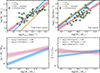 |
Fig. 4. Drivers of the evolution in our scaling relations. The top panels compare how the local TFR and FR (blue curves) would evolve (orange curves) if the only changes are the z evolution of the Hubble parameter and the density contrast, against our high-z data (green markers) and best fits (pink curves). The results imply an evolution of |


At this stage, it is instructive to rearrange Eqs. (11) and (12) as
 (15)
(15)
 (16)
(16)
From these equations, it is clear that fM and fj at any z are entirely specified by the cosmological redshift dependence of the Hubble parameter and density contrast, by fV, and by the observed TFR and FR. The ratio fV depends on the baryonic and dark matter expansion and contraction, but varies only weakly with M* (see Dutton et al. 2010; McGaugh 2012). For instance, Reyes et al. (2012) combined kinematic and weak-lensing observations and found fV ≈ 1.3 − 1.4 for galaxies with 9.8 < log(M*/M⊙) < 10.8 at z = 0. In addition, results from Posti et al. (2019a) and Mancera Piña et al. (2025) on mass models from rotation curve decomposition imply in fV ≈ 1.2 − 1.4 for galaxies with 100 < Vcirc,f/km s−1 < 350. Based on this, and for simplicity, we neglect any M* dependency and consider fV = 1.3 with a 1σ scatter of 0.1. We further assume that fV does not change with z; although no observational constraints exist, idealised models suggest that fV evolves significantly only at z ≳ 2 (Somerville et al. 2008; Dutton et al. 2011).
From the best-fit TFR and FR form this work and Marasco et al. (2025), we compute the resulting ratios, shown in the bottom panels of Fig. 4. Solid lines show the median relations, and the confidence bands the 16th–84th percentile range, derived from the sampling of the best-fitting TFR and FR (including their intrinsic scatter ϵ⊥). For the fM − M* and fj − M* relations at z = 0, the width is around 0.08–0.1 dex. For the z = 0.9 relations, the width is around 0.10–0.13 dex, respectively. For completeness, we also carry out the exercise of propagating the observed vertical scatter in the TFR (σM*) and FR (σj*) into the fM − M* and fj − M* relations. At z = 0, σM* (σj*) propagates into a scatter of 0.16 (0.20) dex at fixed M* (slightly smaller but comparable to literature values, e.g. Romeo et al. 2020, 2023). At z = 0.9, σM* (σj*) propagates into a scatter of 0.20 (0.19) dex at fixed M*. Overall, our redshift comparison reveals changes in fM and fj from z = 0.9 to the present, which we discuss next.
5.2. The evolution of fM
The bottom left panel of Fig. 4 shows fM at z = 0, exhibiting the same single power-law behaviour found for nearby star-forming galaxies based on rotation curve decomposition (e.g. Posti et al. 2019a; Di Teodoro et al. 2023; Mancera Piña et al. 2025). In particular, fM at z = 0 is well described by the expression log(fM) = 0.424log(M*/M⊙)−6.002. On the other hand, at z = 0.9 we find higher fM values for M* < 1012 M⊙ and, crucially, a weaker M* dependency driven by the shallower TFR at z = 0.9, with log(fM) = 0.212log(M*/M⊙)−3.459. The slope of the log(fM)−log(M*) relations at z = 0.9 and z = 0 differ at the same level as the slopes of the TFRs, i.e. around 2σ.
Our observed scaling relations can be used to set interesting constraints in the broader context of galaxy assembly. In particular, we now show that pairing the CDM halo assembly framework with our observational results implies that main-sequence z = 0.9 disc galaxies cannot evolve into the local main-sequence disc population following a simple evolutionary model in which they remain in the SFMS from z = 0.9 to z = 0. To show this schematically, in the top panel of Fig. 5 we construct a simple toy model in which the local fM − M* relation (blue curve) is populated with mock galaxies (circles) and evolved backwards in time to z = 0.9 (squares). The bottom panel recasts the same comparison into the more familiar stellar-to-halo mass plane, highlighting the relative individual growth of M* and Mvir. For this exercise, we assume that the galaxies’ stellar mass evolves following the main sequence star formation rate − M* − z relation of Leja et al. (2022), and that their halo growth follows the halo accretion formalism by van den Bosch et al. (2014). A toy model such as this entails mappings between M*(z = 0.9) and M*(z = 0) and between Mvir(z = 0.9) and Mvir(z = 0) that are monotonic, one-to-one, and rank-order preserving. As a result, the model neglects many complexities of galaxy and halo evolution, as discussed below.
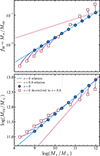 |
Fig. 5. Comparison between our inferred fM − M* (top) and Mvir − M* (bottom) relations and an idealised toy model of mass assembly. The model considers a population of galaxies (blue circles) lying in the z = 0 relations (blue curves), which are then traced back to z = 0.9 (squares), assuming theoretical stellar and halo mass growths. Galaxy downsizing and halo growth histories yield z = 0.9 relations (squares) with slopes different from those observed at z = 0 (solid pink curves). The only way to reconcile the stellar mass growth of galaxies with our inferred relations at z = 0.9 is if low-mass haloes grew more than high-mass haloes since z = 0.9, contrary to CDM expectations. This suggests that the galaxies populating our z = 0.9 relations do not follow this toy model and are unlikely to be the progenitors of the z = 0 population. |
The mass growths implied by such a model yield relations at z = 0.9, which depart from our measurements (pink curves). In general, the bottom panel of Fig. 5 shows that any plausible stellar-mass assembly track would imply a paradoxical, anti-hierarchical growth of DM halos, which would undermine our entire interpretive framework to begin with. This becomes evident when one draws arbitrary evolutionary tracks in M* between the z = 0.9 and z = 0 relations in the bottom panel of Fig. 5, under the minimal assumption that masses do not decrease with time. Independent of the specific increment in M*, massive haloes must already be largely assembled by z = 0.9, while low-mass systems would still be building a substantial fraction of their halo mass at later times7. Such behaviour is at odds with the well-established theoretical expectations in the CDM paradigm, where massive haloes experience stronger fractional growth at late times than their lower-mass counterparts (e.g. Fakhouri et al. 2010; van den Bosch et al. 2014; Correa et al. 2015).
Therefore, we conclude that, if our scaling relations are correct, our main-sequence disc z = 0.9 sample cannot follow the simplified toy model described above, and it is likely not the progenitor of our local main-sequence disc sample (i.e. we are witnessing an example of potential progenitor bias; e.g., van Dokkum & Franx 1996, 2001). This is perhaps not surprising, as the idealised toy model above does not capture processes such as mergers, feedback, star-formation bursts, and quenching, all of which can lead to morphological transformations (Cimatti et al. 2019), which our results suggest are in place.
As another option, we can consider the possibility that our observed scaling relations are incorrect. As shown in the top-left panel of Fig. 4, reconciling the z = 0.9 TFR with the cosmology-only halo scaling hypothesis (i.e. assuming no evolution of fM) would mean that the circular speeds of galaxies with log(M*/M⊙)≲10.7 have been underestimated by ∼50%. As discussed extensively in Sect. 4.3, the uncertainties considered in this work appear to be insufficient to account for this discrepancy on their own. Another possibility is that strong selection-function effects, additional unknown systematic effects, or inappropriate assumptions may bias our results. Crucially, we note that such effects must have also been present in previous TFR determinations at z ∼ 1, which report slopes consistent with ours (see Sect. 4.1). Alternatively, one may be inclined to conclude that ionised gas kinematics cannot be used to infer dynamical properties of high-z star-forming galaxies, regardless of a careful approach such as ours, which includes robust 3D kinematic modelling, AD corrections, Sérsic modelling of NIR data, and homogeneous stellar mass determinations. On the theoretical side, this should be further explored through simulations that track the evolution of individual galaxies. On the observational side, it would be key to trace the TFR and FR across finer redshift intervals and to earlier epochs. Upcoming facilities such as SKA, ALMA, Euclid, and Roman will also provide direct constraints on galaxy kinematics and halo properties through deep cold-gas observations and weak-lensing measurements, and will be key to obtaining a more definitive picture.
Finally, we would like to highlight the recent studies based on abundance matching and angular clustering by Shuntov et al. (2025) and Paquereau et al. (2025), respectively. Looking at the COSMOS field with JWST, the above authors also find tentative evidence of higher values of fM at z ∼ 1 than at z ∼ 0, though no explanation has yet been offered. This is unlike previous abundance-matching studies8, which typically suggest a higher fM at z = 0 than at z = 1, with only mild evolution in slope (Moster et al. 2010). State-of-the-art hydrodynamical simulations generally show little redshift evolution in fM (Chaikin et al. 2025), so clearly obtaining additional observational constraints will be key.
5.3. The evolution of fj and fR
Next, we turn our attention to fj, shown in the bottom right panel of Fig. 4. At both redshifts, fj depends more weakly on M* than fM (see also e.g. Posti et al. 2019b; Di Teodoro et al. 2023; Romeo et al. 2023). Within our mass coverage, fj ∼ 0.8, in agreement with previous studies (e.g. Fall & Romanowsky 2013, 2018; Posti et al. 2019b; Di Teodoro et al. 2023). Specifically, within 9.5 < log(M*/M⊙) < 11.5, fM at z = 0 increases by a factor of ∼2, while at z = 0.9 it decreases by 30%. The fj − M* relations are well described by the power laws log(fj) = 0.141log(M*/M⊙)−1.695 at z = 0, and log(fj) = − 0.079log(M*/M⊙)+0.757 at z = 0.9.
Taken at face value, our results indicate that disc galaxies with log(M*/M⊙)≲11.1 have lowered their fj over the last ∼8 Gyr and more massive galaxies have raised it, but the overall redshift and mass dependence is weak. Since fj depends indirectly on fM through the TFR ( ; see Eq. (16)), it is instructive to explore a limiting case in which fM does not evolve. In this scenario, the evolution of fj arises exclusively from the Hubble parameter, the density contrast, and the FR. This assumption is not fully self-consistent, as it requires that our measurements trace V* but not Vcirc, f. Nevertheless, it is helpful as a hypothetical exercise to test whether an evolution of fj remains. The results are shown in the bottom-right panel of Fig. 4 as a dashed grey curve. The imposed steeper fM-M* relation flips the sign of the fj-M* slope, though the dependence on M* remains weak. As already suggested by the orange curve in the top-right panel of Fig. 4 (if fM and fj do not evolve with z the observed FR is not reproduced), the conservative scenario of no evolution in fM still results in an evolution of fj, though it is relatively mild.
Different mechanisms can increase or decrease fj as a function of M* and z, such as outflows, galactic fountains, stripping, mergers, and dynamical friction (e.g. van den Bosch et al. 2001; Brook et al. 2012; Romanowsky & Fall 2012; Lagos et al. 2017; Irodotou et al. 2019). For instance, feedback-driven outflows near galaxy centres can lead to a larger fj (Brook et al. 2011; Romanowsky & Fall 2012). In addition, the cumulative effect of dry mergers between z = 0.9 to z = 0 could reduce fj at z = 0 relative to z = 0.9 (Fall 1979; Romanowsky & Fall 2012; Lagos et al. 2018). A combination of these different phenomena could explain the behaviour of fj in the bottom right panel of Fig. 4. Yet, establishing the precise mechanisms would require a more accurate determination of fj, coupled with analysis of hydrodynamical simulations. Overall, the lack of a strong z or M* dependence of fj suggests that the above processes are gentle (or compensated each other) from z = 0.9 to z = 0.
Our results also have immediate implications for the relative sizes of galaxy discs compared to their host haloes. For exponential discs (a good approximation for our sample; see Fig. 1) embedded in SIS haloes, one obtains  (e.g. Fall & Efstathiou 1980; Fall 1983; see also Mo et al. 1998 for the NFW case). For fV = 1.3, this reduces to fR ≈ 0.032 fj, so that the evolution of fR(M*, z) is fully specified by that of fj(M*, z) in Fig. 4. Our finding of only weak variation in fR(M*, z) agrees well with previous semi-empirical studies (e.g. combining observed galaxy sizes with abundance-matching halo sizes; Huang et al. 2017; Somerville et al. 2018) and with results from hydrodynamical simulations (Grand et al. 2017; Rodriguez-Gomez et al. 2022; Somerville et al. 2025).
5.4. A short remark on gas content
An important aspect to keep in mind is that throughout this study, we have only considered the stellar component of fM and fj, since resolved cold gas measurements at z ∼ 1 remain scarce (for indirect estimates see e.g. Puech et al. 2010), partly due to gaps between ALMA bands. Yet, at z = 0 it is well established that cold gas carries a substantial fraction of the angular momentum budget and contributes significantly to the baryonic j of galaxies, except in the most massive discs (e.g. Mancera Piña et al. 2021a,b; Romeo et al. 2023). Moreover, the baryon-to-halo mass relation is shallower than the stellar one at z = 0 (Romeo et al. 2023; Mancera Piña et al. 2025), and the higher cold gas fractions at earlier epochs (Tacconi et al. 2020) make this even more relevant at z ∼ 1.
Additionally, cold gas kinematics would help reduce the observational uncertainties in our analysis (see Sect. 3), enabling a more robust reassessment of the evolution of the baryon-to-halo mass and angular momentum ratios. Evidently, incorporating the cold gas reservoir is crucial for an integral picture of the evolution of fM and fj.
Beyond the cold gas in discs, a complete understanding of the drivers of fM and fj also requires accounting for the circumgalactic medium and large-scale cold gas, both of which can exchange angular momentum with galaxies. Recent studies have explored this using advanced models and simulations (e.g. Pezzulli et al. 2017; Afruni et al. 2022; Wang et al. 2022; Afruni et al. 2023; Liu et al. 2025; Simons et al. 2025; Wang et al. 2025), but connecting these predictions to observations remains a key challenge for the years to come.
6. Summary and conclusions
In this work, we have built the Tully-Fisher (M* − Vcirc, f, TFR) and Fall (j* − M*, FR) relations for a sample of disc galaxies at z = 0.9. To do so, we first compiled a sample of galaxies with public IFU Hα kinematic data and space-based (JWST and HST) imaging. We applied different quality cuts, resulting in a high-quality sample of 43 star-forming rotationally supported discs (Fig. 1) with 5 × 10⁹ < M*/M⊙ < 2 × 10¹¹ and 0.78 < z < 1.03, encompassing a cosmic time when the Universe was half its current age. The galaxies in our sample have representative star formation rates, Sérsic indices, and effective radii across our M* and z ranges.
We derived robust kinematic models (Fig. A.1) that enabled us to retrieve the intrinsic kinematics of the galaxies, despite the low spatial resolution, thereby improving upon previous literature. To account for the pressure-supported motions in our galaxies, we computed realistic asymmetric drift corrections, which allowed us to convert our measured Hα rotational velocities into circular speeds (whose flat value Vcirc, f enters the TFR) and stellar rotational velocities (V*, which is needed to compute j* for the FR).
Paired with spatial and spectral modelling of JWST and HST data, we measured M*, j*, and Vcirc, f (in a consistent way as done at z = 0), and we determined the z = 0.9 TFR and FR (Fig. 2, see also Fig. A.3). We parametrised the observed trends with power-laws (Fig. 2 and Table 1). We note that the asymmetric drift corrections have a non-negligible impact on the best-fitting TFR and FR, highlighting the importance of applying them.
By comparing our best-fitting relations with a recent determination in the nearby Universe based on cold neutral atomic gas, we detected moderate evolution of the TFR and a more substantial evolution of the FR (Fig. 3). At z = 0.9, the TFR has a shallower mass dependency and a higher intercept. On the other hand, the FR has a slightly shallower slope and an intercept about 0.2 dex lower. We discussed in detail different caveats that could affect the determination of our relations, finding that our results are robust against the presence of potential known systematics (but see below), unless the TFR and FR are not intrinsically unbroken power laws.
A key aspect of this study is that we connected the observed TFR and FR with scaling relations for dark matter haloes. We found that the evolution of the relations cannot be explained by a model where the z = 0 TFR and FR are evolved to z = 0.9 by accounting for the z evolution of the Hubble parameter and density contrast alone (Fig. 4, top panels), but instead requires intrinsic variations in the galaxy mass and angular momentum assembly histories. Specifically, the quantities  and
and  must evolve with z, with fV = Vcirc, f/Vvir, fM = M*/Mvir, and fj = j*/jvir. Choosing a realistic fV, we showed the dependencies that fM and fj should have as a function of M* and z given our TFR and FR (Fig. 4, bottom panels). This represents a significant improvement in the literature studying the fM and fj ratios, which often assume abundance-matching values rather than deriving them directly from the data. At z = 0, we found that both fM and fj increase with stellar mass, in agreement with previous observations.
Our results show that, within the CDM framework, the observed scaling relations are incompatible with a simple evolutionary model in which our main-sequence disc z = 0.9 population becomes the progenitor of the main-sequence disc z = 0 population (Fig. 5), implying a more complex morphological transformation and baryonic mass assembly instead. Alternatively, it could be that our scaling relations are incorrect due to extreme selection effects, large unrecognised systematics, severely flawed assumptions in our or previous works, or the possibility that ionised-gas kinematics is not a reliable dynamical tracer.
As for fj, we found its normalisation to be slightly higher at z = 0.9 across most of our M* range. However, the overall variation with M* and z is weak, which sets constraints on the different processes that can increase or decrease fj during galaxy formation. The evolution of fj also determines the evolution of the ratio fR = Reff, */Rvir ≈ 0.032 fj. Accordingly, we found relatively little evolution on fR(M*, z), in agreement with previous theoretical and semi-empirical determinations.
Besides an improvement in the quality of kinematic data, the study of the time evolution of fM and fj needs to be complemented with models and simulations that incorporate the complexity of galaxy evolution in a cosmological context (e.g. Sales et al. 2009; Dutton & van den Bosch 2012; Genel et al. 2015; Pedrosa & Tissera 2015; Teklu et al. 2015; Grand et al. 2017; Lagos et al. 2017; El-Badry et al. 2018; Rodriguez-Gomez et al. 2022; Yang et al. 2024). Our observational results serve as vital benchmarks for such theoretical models.
Acknowledgments
We thank the referee for helpful comments and feedback. We thank Joop Schaye, Filippo Fraternali, Francesca Rizzo, Pieter van Dokkum, and Marijn Franx for valuable comments and discussions. We also thank Christopher Harrison and Mark Swinbank for their clarifications on the KROSS data, Arjen van der Wel for his assistance on Sérsic models, and Henk Hoekstra for clarifications on weak-lensing estimates. PEMP is funded by the Dutch Research Council (NWO) through the Veni grant VI.Veni.222.364. EDT was supported by the European Research Council (ERC) under grant agreement no. 101040751. We have used the services from SIMBAD, NED, and ADS extensively, as well as the tool TOPCAT (Taylor 2005) and the Python packages NumPy (Oliphant 2007), Matplotlib (Hunter 2007), SciPy (Virtanen et al. 2020), and Astropy (Astropy Collaboration 2018), for which we are thankful.
References
- Abril-Melgarejo, V., Epinat, B., Mercier, W., et al. 2021, A&A, 647, A152 [NASA ADS] [CrossRef] [EDP Sciences] [Google Scholar]
- Afruni, A., Pezzulli, G., & Fraternali, F. 2022, MNRAS, 509, 4849 [Google Scholar]
- Afruni, A., Pezzulli, G., Fraternali, F., & Grønnow, A. 2023, MNRAS, 524, 2351 [NASA ADS] [CrossRef] [Google Scholar]
- Alcorn, L. Y., Tran, K.-V., Glazebrook, K., et al. 2018, ApJ, 858, 47 [NASA ADS] [CrossRef] [Google Scholar]
- Araujo-Carvalho, A. E., Gonçalves, T. S., Krajnović, D., Menéndez-Delmestre, K., & de Isídio, N. 2025, ApJ, 991, 3 [Google Scholar]
- Astropy Collaboration (Price-Whelan, A. M., et al.) 2018, AJ, 156, 123 [Google Scholar]
- Bell, E. F., & de Jong, R. S. 2001, ApJ, 550, 212 [Google Scholar]
- Bett, P., Eke, V., Frenk, C. S., et al. 2007, MNRAS, 376, 215 [NASA ADS] [CrossRef] [Google Scholar]
- Binney, J. 1977, ApJ, 215, 483 [NASA ADS] [CrossRef] [Google Scholar]
- Binney, J., & Tremaine, S. 2008, Galactic Dynamics: Second Edition [Google Scholar]
- Blumenthal, G. R., Faber, S. M., Primack, J. R., & Rees, M. J. 1984, Nature, 311, 517 [Google Scholar]
- Bouché, N. F., Genel, S., Pellissier, A., et al. 2021, A&A, 654, A49 [NASA ADS] [CrossRef] [EDP Sciences] [Google Scholar]
- Brook, C. B., Governato, F., Roškar, R., et al. 2011, MNRAS, 415, 1051 [NASA ADS] [CrossRef] [Google Scholar]
- Brook, C. B., Stinson, G., Gibson, B. K., et al. 2012, MNRAS, 419, 771 [NASA ADS] [CrossRef] [Google Scholar]
- Bruzual, G., & Charlot, S. 2003, MNRAS, 344, 1000 [NASA ADS] [CrossRef] [Google Scholar]
- Bryan, G. L., & Norman, M. L. 1998, ApJ, 495, 80 [NASA ADS] [CrossRef] [Google Scholar]
- Bullock, J. S., Dekel, A., Kolatt, T. S., et al. 2001, ApJ, 555, 240 [NASA ADS] [CrossRef] [Google Scholar]
- Burkert, A., Förster Schreiber, N. M., Genzel, R., et al. 2016, ApJ, 826, 214 [Google Scholar]
- Carnall, A. C., McLure, R. J., Dunlop, J. S., & Davé, R. 2018, MNRAS, 480, 4379 [Google Scholar]
- Casey, C. M., Kartaltepe, J. S., Drakos, N. E., et al. 2023, ApJ, 954, 31 [NASA ADS] [CrossRef] [Google Scholar]
- Catinella, B., Cortese, L., Tiley, A. L., et al. 2023, MNRAS, 519, 1098 [Google Scholar]
- Chaikin, E., Schaye, J., Schaller, M., et al. 2025, arXiv e-prints [arXiv:2509.07960] [Google Scholar]
- Charlot, S., & Fall, S. M. 2000, ApJ, 539, 718 [Google Scholar]
- Cimatti, A., Fraternali, F., & Nipoti, C. 2019, Introduction to Galaxy Formation and Evolution: From Primordial Gas to Present-Day Galaxies (Cambridge University Press) [Google Scholar]
- Conselice, C. J., Bundy, K., Ellis, R. S., et al. 2005, ApJ, 628, 160 [Google Scholar]
- Contini, T., Epinat, B., Bouché, N., et al. 2016, A&A, 591, A49 [NASA ADS] [CrossRef] [EDP Sciences] [Google Scholar]
- Correa, C. A., Wyithe, J. S. B., Schaye, J., & Duffy, A. R. 2015, MNRAS, 452, 1217 [CrossRef] [Google Scholar]
- Cortese, L., Fogarty, L. M. R., Bekki, K., et al. 2016, MNRAS, 463, 170 [NASA ADS] [CrossRef] [Google Scholar]
- Courteau, S., Dutton, A. A., van den Bosch, F. C., et al. 2007, ApJ, 671, 203 [Google Scholar]
- Cresci, G., Hicks, E. K. S., Genzel, R., et al. 2009, ApJ, 697, 115 [Google Scholar]
- Dalcanton, J. J., Spergel, D. N., & Summers, F. J. 1997, ApJ, 482, 659 [NASA ADS] [CrossRef] [Google Scholar]
- Di Teodoro, E. M., & Fraternali, F. 2015, MNRAS, 451, 3021 [Google Scholar]
- Di Teodoro, E. M., & Peek, J. E. G. 2021, ApJ, 923, 220 [NASA ADS] [CrossRef] [Google Scholar]
- Di Teodoro, E. M., Fraternali, F., & Miller, S. H. 2016, A&A, 594, A77 [NASA ADS] [CrossRef] [EDP Sciences] [Google Scholar]
- Di Teodoro, E. M., Posti, L., Ogle, P. M., Fall, S. M., & Jarrett, T. 2021, MNRAS, 507, 5820 [NASA ADS] [CrossRef] [Google Scholar]
- Di Teodoro, E. M., Posti, L., Fall, S. M., et al. 2023, MNRAS, 518, 6340 [Google Scholar]
- Dunlop, J. S., Abraham, R. G., Ashby, M. L. N., et al. 2021, PRIMER: Public Release IMaging for Extragalactic Research, JWST Proposal. Cycle 1, ID. #1837 [Google Scholar]
- Dutton, A. A., & van den Bosch, F. C. 2012, MNRAS, 421, 608 [NASA ADS] [Google Scholar]
- Dutton, A. A., Conroy, C., van den Bosch, F. C., Prada, F., & More, S. 2010, MNRAS, 407, 2 [Google Scholar]
- Dutton, A. A., van den Bosch, F. C., Faber, S. M., et al. 2011, MNRAS, 410, 1660 [NASA ADS] [Google Scholar]
- Eisenstein, D. J., Willott, C., Alberts, S., et al. 2023, arXiv e-prints [arXiv:2306.02465] [Google Scholar]
- Ejdetjärn, T., Agertz, O., Östlin, G., Renaud, F., & Romeo, A. B. 2022, MNRAS, 514, 480 [CrossRef] [Google Scholar]
- El-Badry, K., Quataert, E., Wetzel, A., et al. 2018, MNRAS, 473, 1930 [NASA ADS] [CrossRef] [Google Scholar]
- Eldridge, J. J., & Stanway, E. R. 2009, MNRAS, 400, 1019 [NASA ADS] [CrossRef] [Google Scholar]
- Espejo Salcedo, J. M., Glazebrook, K., Fisher, D. B., et al. 2025, MNRAS, 536, 1188 [Google Scholar]
- Fakhouri, O., Ma, C.-P., & Boylan-Kolchin, M. 2010, MNRAS, 406, 2267 [Google Scholar]
- Fall, S. M. 1979, Nature, 281, 200 [NASA ADS] [CrossRef] [Google Scholar]
- Fall, S. M. 1983, IAU Symp., 100, 391 [Google Scholar]
- Fall, S. M., & Efstathiou, G. 1980, MNRAS, 193, 189 [NASA ADS] [CrossRef] [Google Scholar]
- Fall, S. M., & Romanowsky, A. J. 2013, ApJ, 769, L26 [Google Scholar]
- Fall, S. M., & Romanowsky, A. J. 2018, ApJ, 868, 133 [Google Scholar]
- Forbes, D. A., & Gannon, J. 2024, MNRAS, 528, 608 [NASA ADS] [CrossRef] [Google Scholar]
- Fouque, P., Bottinelli, L., Gouguenheim, L., & Paturel, G. 1990, ApJ, 349, 1 [CrossRef] [Google Scholar]
- Fraternali, F., Karim, A., Magnelli, B., et al. 2021, A&A, 647, A194 [NASA ADS] [CrossRef] [EDP Sciences] [Google Scholar]
- Geesink, N. N., Mancera Piña, P. E., Lagos, C. d. P., & Kriek, M. 2025, A&A, 697, A87 [NASA ADS] [CrossRef] [EDP Sciences] [Google Scholar]
- Genel, S., Fall, S. M., Hernquist, L., et al. 2015, ApJ, 804, L40 [NASA ADS] [CrossRef] [Google Scholar]
- Gillman, S., Swinbank, A. M., Tiley, A. L., et al. 2019, MNRAS, 486, 175 [NASA ADS] [CrossRef] [Google Scholar]
- Gillman, S., Tiley, A. L., Swinbank, A. M., et al. 2020, MNRAS, 492, 1492 [Google Scholar]
- Girard, M., Fisher, D. B., Bolatto, A. D., et al. 2021, ApJ, 909, 12 [NASA ADS] [CrossRef] [Google Scholar]
- Grand, R. J. J., Gómez, F. A., Marinacci, F., et al. 2017, MNRAS, 467, 179 [NASA ADS] [Google Scholar]
- Grogin, N. A., Kocevski, D. D., Faber, S. M., et al. 2011, ApJS, 197, 35 [NASA ADS] [CrossRef] [Google Scholar]
- Hardwick, J. A., Cortese, L., Obreschkow, D., Catinella, B., & Cook, R. H. W. 2022, MNRAS, 509, 3751 [Google Scholar]
- Harrison, C. M., Johnson, H. L., Swinbank, A. M., et al. 2017, MNRAS, 467, 1965 [Google Scholar]
- Huang, K.-H., Fall, S. M., Ferguson, H. C., et al. 2017, ApJ, 838, 6 [NASA ADS] [CrossRef] [Google Scholar]
- Hubble, E. P. 1926, ApJ, 64, 321 [Google Scholar]
- Hunter, J. D. 2007, Comput. Sci. Eng., 9, 90 [NASA ADS] [CrossRef] [Google Scholar]
- Irodotou, D., Thomas, P. A., Henriques, B. M., Sargent, M. T., & Hislop, J. M. 2019, MNRAS, 489, 3609 [NASA ADS] [Google Scholar]
- Koekemoer, A. M., Aussel, H., Calzetti, D., et al. 2007, ApJS, 172, 196 [Google Scholar]
- Koekemoer, A. M., Faber, S. M., Ferguson, H. C., et al. 2011, ApJS, 197, 36 [NASA ADS] [CrossRef] [Google Scholar]
- Kroupa, P. 2002, Science, 295, 82 [Google Scholar]
- Lagos, C. d. P., Theuns, T., Stevens, A. R. H., et al. 2017, MNRAS, 464, 3850 [Google Scholar]
- Lagos, C. d. P., Stevens, A. R. H., Bower, R. G., et al. 2018, MNRAS, 473, 4956 [Google Scholar]
- Leja, J., Speagle, J. S., Ting, Y.-S., et al. 2022, ApJ, 936, 165 [NASA ADS] [CrossRef] [Google Scholar]
- Lelli, F., McGaugh, S. S., & Schombert, J. M. 2016, AJ, 152, 157 [Google Scholar]
- Levy, R. C., Bolatto, A. D., Teuben, P., et al. 2018, ApJ, 860, 92 [NASA ADS] [CrossRef] [Google Scholar]
- Liu, K., Guo, H., Wang, S., et al. 2025, A&A, 693, A48 [NASA ADS] [CrossRef] [EDP Sciences] [Google Scholar]
- Mancera Piña, P. E., Fraternali, F., Oman, K. A., et al. 2020, MNRAS, 495, 3636 [Google Scholar]
- Mancera Piña, P. E., Posti, L., Fraternali, F., Adams, E. A. K., & Oosterloo, T. 2021a, A&A, 647, A76 [NASA ADS] [CrossRef] [EDP Sciences] [Google Scholar]
- Mancera Piña, P. E., Posti, L., Pezzulli, G., et al. 2021b, A&A, 651, L15 [NASA ADS] [CrossRef] [EDP Sciences] [Google Scholar]
- Mancera Piña, P. E., Fraternali, F., Oosterloo, T., et al. 2022, MNRAS, 514, 3329 [CrossRef] [Google Scholar]
- Mancera Piña, P. E., Golini, G., Trujillo, I., & Montes, M. 2024, A&A, 689, A344 [NASA ADS] [CrossRef] [EDP Sciences] [Google Scholar]
- Mancera Piña, P. E., Read, J. I., Kim, S., et al. 2025, A&A, 699, A311 [NASA ADS] [CrossRef] [EDP Sciences] [Google Scholar]
- Marasco, A., Fraternali, F., Posti, L., et al. 2019, A&A, 621, L6 [NASA ADS] [CrossRef] [EDP Sciences] [Google Scholar]
- Marasco, A., Posti, L., Oman, K., et al. 2020, A&A, 640, A70 [EDP Sciences] [Google Scholar]
- Marasco, A., Fall, S. M., Di Teodoro, E. M., & Mancera Piña, P. E. 2025, A&A, 695, L23 [NASA ADS] [CrossRef] [EDP Sciences] [Google Scholar]
- Martinsson, T. P. K., Verheijen, M. A. W., Westfall, K. B., et al. 2013, A&A, 557, A130 [NASA ADS] [CrossRef] [EDP Sciences] [Google Scholar]
- Martorano, M., van der Wel, A., Bell, E. F., et al. 2023, ApJ, 957, 46 [NASA ADS] [CrossRef] [Google Scholar]
- Martorano, M., van der Wel, A., Baes, M., et al. 2024, ApJ, 972, 134 [Google Scholar]
- Martorano, M., van der Wel, A., Gebek, A., et al. 2026, A&A, in press, https://doi.org/10.1051/0004-6361/202555974 [Google Scholar]
- McGaugh, S. S. 2012, AJ, 143, 40 [Google Scholar]
- Mercier, W., Epinat, B., Contini, T., et al. 2023, A&A, 677, A143 [NASA ADS] [CrossRef] [EDP Sciences] [Google Scholar]
- Mo, H. J., Mao, S., & White, S. D. M. 1998, MNRAS, 295, 319 [Google Scholar]
- Mogotsi, K. M., & Romeo, A. B. 2019, MNRAS, 489, 3797 [Google Scholar]
- Moster, B. P., Somerville, R. S., Maulbetsch, C., et al. 2010, ApJ, 710, 903 [Google Scholar]
- Navarro, J. F., Frenk, C. S., & White, S. D. M. 1997, ApJ, 490, 493 [Google Scholar]
- Nelson, E. J., van Dokkum, P. G., Brammer, G., et al. 2012, ApJ, 747, L28 [CrossRef] [Google Scholar]
- Nelson, E. J., van Dokkum, P. G., Förster Schreiber, N. M., et al. 2016, ApJ, 828, 27 [Google Scholar]
- Obreschkow, D., & Glazebrook, K. 2014, ApJ, 784, 26 [Google Scholar]
- Obreschkow, D., Meyer, M., Popping, A., et al. 2015, in Advancing Astrophysics with the Square Kilometre Array (AASKA14), 138 [Google Scholar]
- Oliphant, T. E. 2007, Comput. Sci. Eng., 9, 10 [NASA ADS] [CrossRef] [Google Scholar]
- Paquereau, L., Laigle, C., McCracken, H. J., et al. 2025, A&A, 702, A163 [NASA ADS] [CrossRef] [EDP Sciences] [Google Scholar]
- Pedrosa, S. E., & Tissera, P. B. 2015, A&A, 584, A43 [NASA ADS] [CrossRef] [EDP Sciences] [Google Scholar]
- Peebles, P. J. E. 1969, ApJ, 155, 393 [Google Scholar]
- Pelliccia, D., Lemaux, B. C., Tomczak, A. R., et al. 2019, MNRAS, 482, 3514 [Google Scholar]
- Peng, C. Y., Ho, L. C., Impey, C. D., & Rix, H.-W. 2010, AJ, 139, 2097 [Google Scholar]
- Pezzulli, G., Fraternali, F., & Binney, J. 2017, MNRAS, 467, 311 [NASA ADS] [Google Scholar]
- Ponomareva, A. A., Verheijen, M. A. W., Peletier, R. F., & Bosma, A. 2017, MNRAS, 469, 2387 [NASA ADS] [CrossRef] [Google Scholar]
- Posti, L., Fraternali, F., Di Teodoro, E. M., & Pezzulli, G. 2018, A&A, 612, L6 [NASA ADS] [CrossRef] [EDP Sciences] [Google Scholar]
- Posti, L., Fraternali, F., & Marasco, A. 2019a, A&A, 626, A56 [NASA ADS] [CrossRef] [EDP Sciences] [Google Scholar]
- Posti, L., Marasco, A., Fraternali, F., & Famaey, B. 2019b, A&A, 629, A59 [NASA ADS] [CrossRef] [EDP Sciences] [Google Scholar]
- Price, S. H., Kriek, M., Shapley, A. E., et al. 2016, ApJ, 819, 80 [Google Scholar]
- Puech, M., Hammer, F., Flores, H., et al. 2010, A&A, 510, A68 [NASA ADS] [CrossRef] [EDP Sciences] [Google Scholar]
- Reyes, R., Mandelbaum, R., Gunn, J. E., Pizagno, J., & Lackner, C. N. 2011, MNRAS, 417, 2347 [Google Scholar]
- Reyes, R., Mandelbaum, R., Gunn, J. E., et al. 2012, MNRAS, 425, 2610 [NASA ADS] [CrossRef] [Google Scholar]
- Rizzo, F., Kohandel, M., Pallottini, A., et al. 2022, A&A, 667, A5 [NASA ADS] [CrossRef] [EDP Sciences] [Google Scholar]
- Rizzo, F., Roman-Oliveira, F., Fraternali, F., et al. 2023, A&A, 679, A129 [NASA ADS] [CrossRef] [EDP Sciences] [Google Scholar]
- Rodriguez-Gomez, V., Sales, L. V., Genel, S., et al. 2017, MNRAS, 467, 3083 [Google Scholar]
- Rodriguez-Gomez, V., Genel, S., Fall, S. M., et al. 2022, MNRAS, 512, 5978 [NASA ADS] [CrossRef] [Google Scholar]
- Romanowsky, A. J., & Fall, S. M. 2012, ApJS, 203, 17 [Google Scholar]
- Romeo, A. B., Agertz, O., & Renaud, F. 2020, MNRAS, 499, 5656 [NASA ADS] [CrossRef] [Google Scholar]
- Romeo, A. B., Agertz, O., & Renaud, F. 2023, MNRAS, 518, 1002 [Google Scholar]
- Rowland, L. E., Hodge, J., Bouwens, R., et al. 2024, MNRAS, 535, 2068 [Google Scholar]
- Sales, L. V., Navarro, J. F., Schaye, J., et al. 2009, MNRAS, 399, L64 [NASA ADS] [Google Scholar]
- Schombert, J., McGaugh, S., & Lelli, F. 2022, AJ, 163, 154 [NASA ADS] [CrossRef] [Google Scholar]
- Scoville, N., Aussel, H., Brusa, M., et al. 2007, ApJS, 172, 1 [Google Scholar]
- Sharma, G., Salucci, P., Harrison, C. M., van de Ven, G., & Lapi, A. 2021, MNRAS, 503, 1753 [CrossRef] [Google Scholar]
- Sharma, G., Upadhyaya, V., Salucci, P., & Desai, S. 2024, A&A, 689, A318 [NASA ADS] [CrossRef] [EDP Sciences] [Google Scholar]
- Sharma, G., van de Ven, G., Salucci, P., & Martorano, M. 2025, A&A, 699, A164 [NASA ADS] [CrossRef] [EDP Sciences] [Google Scholar]
- Shuntov, M., Ilbert, O., Toft, S., et al. 2025, A&A, 695, A20 [NASA ADS] [CrossRef] [EDP Sciences] [Google Scholar]
- Simons, R. C., Peeples, M. S., Tumlinson, J., et al. 2025, ApJ, 988, 250 [Google Scholar]
- Somerville, R. S., Barden, M., Rix, H.-W., et al. 2008, ApJ, 672, 776 [NASA ADS] [CrossRef] [Google Scholar]
- Somerville, R. S., Behroozi, P., Pandya, V., et al. 2018, MNRAS, 473, 2714 [NASA ADS] [CrossRef] [Google Scholar]
- Somerville, R. S., Gabrielpillai, A., Hadzhiyska, B., & Genel, S. 2025, arXiv e-prints [arXiv:2502.03679] [Google Scholar]
- Speagle, J. S. 2020, MNRAS, 493, 3132 [Google Scholar]
- Stanway, E. R., & Eldridge, J. J. 2018, MNRAS, 479, 75 [NASA ADS] [CrossRef] [Google Scholar]
- Stevens, A. R. H., Croton, D. J., & Mutch, S. J. 2016, MNRAS, 461, 859 [Google Scholar]
- Stott, J. P., Swinbank, A. M., Johnson, H. L., et al. 2016, MNRAS, 457, 1888 [Google Scholar]
- Suess, K. A., Bezanson, R., Nelson, E. J., et al. 2022, ApJ, 937, L33 [NASA ADS] [CrossRef] [Google Scholar]
- Swaters, R. A. 1999, Ph.D. Thesis, Kapteyn Astronomical Institute, University of Groningen [Google Scholar]
- Sweet, S. M., Fisher, D. B., Savorgnan, G., et al. 2019, MNRAS, 485, 5700 [NASA ADS] [CrossRef] [Google Scholar]
- Sweet, S. M., Glazebrook, K., Obreschkow, D., et al. 2020, MNRAS, 494, 5421 [NASA ADS] [CrossRef] [Google Scholar]
- Swinbank, A. M., Harrison, C. M., Trayford, J., et al. 2017, MNRAS, 467, 3140 [NASA ADS] [Google Scholar]
- Tacconi, L. J., Genzel, R., & Sternberg, A. 2020, ARA&A, 58, 157 [NASA ADS] [CrossRef] [Google Scholar]
- Taylor, M. B. 2005, ASP Conf. Ser., 347, 29 [Google Scholar]
- Teklu, A. F., Remus, R.-S., Dolag, K., et al. 2015, ApJ, 812, 29 [Google Scholar]
- Tiley, A. L., Bureau, M., Cortese, L., et al. 2019, MNRAS, 482, 2166 [Google Scholar]
- Tully, R. B., & Fisher, J. R. 1977, A&A, 500, 105 [Google Scholar]
- Übler, H., Förster Schreiber, N. M., Genzel, R., et al. 2017, ApJ, 842, 121 [Google Scholar]
- van den Bosch, F. C., Burkert, A., & Swaters, R. A. 2001, MNRAS, 326, 1205 [NASA ADS] [CrossRef] [Google Scholar]
- van den Bosch, F. C., Jiang, F., Hearin, A., et al. 2014, MNRAS, 445, 1713 [NASA ADS] [CrossRef] [Google Scholar]
- van der Kruit, P. C. 1988, A&A, 192, 117 [NASA ADS] [Google Scholar]
- van der Wel, A., Bell, E. F., Häussler, B., et al. 2012, ApJS, 203, 24 [NASA ADS] [CrossRef] [Google Scholar]
- van der Wel, A., Chang, Y.-Y., Bell, E. F., et al. 2014, ApJ, 792, L6 [NASA ADS] [CrossRef] [Google Scholar]
- van Dokkum, P. G., & Franx, M. 1996, MNRAS, 281, 985 [NASA ADS] [CrossRef] [Google Scholar]
- van Dokkum, P. G., & Franx, M. 2001, ApJ, 553, 90 [NASA ADS] [CrossRef] [Google Scholar]
- Virtanen, P., Gommers, R., Oliphant, T. E., et al. 2020, Nat. Methods, 17, 261 [Google Scholar]
- Wang, S., Xu, D., Lu, S., et al. 2022, MNRAS, 509, 3148 [Google Scholar]
- Wang, S., Xu, D., & Lu, S. 2025, ApJ, 986, 85 [Google Scholar]
- White, S. D. M. 1984, ApJ, 286, 38 [NASA ADS] [CrossRef] [Google Scholar]
- White, S. D. M., & Rees, M. J. 1978, MNRAS, 183, 341 [Google Scholar]
- Wilman, D. J., Fossati, M., Mendel, J. T., et al. 2020, ApJ, 892, 1 [NASA ADS] [CrossRef] [Google Scholar]
- Wisnioski, E., Förster Schreiber, N. M., Wuyts, S., et al. 2015, ApJ, 799, 209 [Google Scholar]
- Wisnioski, E., Förster Schreiber, N. M., Fossati, M., et al. 2019, ApJ, 886, 124 [Google Scholar]
- Yang, H., Liao, S., Fattahi, A., et al. 2024, MNRAS, 535, 1394 [Google Scholar]
We also explored the BPASS stellar population models (Eldridge & Stanway 2009; Stanway & Eldridge 2018), finding that they produce stellar masses lower 0.25 dex on average but without significant systematics, and therefore do not affect the slopes of the scaling relations presented in Sect. 4.1.
Our median rotation-to-dispersion ratio Vf/σHα, med is close to 5 (see Appendix A), where σHα, med is the median Hα velocity dispersion radial profile. Since σHα is typically twice that of the cold gas (Levy et al. 2018; Girard et al. 2021; Ejdetjärn et al. 2022), this correction would align Vf/σHα, med with typical values observed at z = 0 in disc galaxies with cold gas kinematics (e.g. Mancera Piña et al. 2025).
We have modified the relation from van der Wel et al. (2014) to account for typical differences between their optical sizes and NIR sizes (used in Martorano et al. 2024 and this work). Specifically, we rescaled the optical sizes by linear interpolation so that they decrease by 0.1 dex at log(M*/M⊙) = 9.5 and by 0.22 dex at log(M*/M⊙) = 11.3, consistent with Martorano et al. (2024, see their Fig. 7).
Vcirc(R) is the speed of a test particle in pure circular orbit at a radius R, e.g. Binney & Tremaine (2008), Cimatti et al. (2019). Vcirc is close to the rotational speed of H I, typically used at z = 0 to derive the TFR.
This was done for simplicity and to avoid over-interpreting the data. For some galaxies, σHα(R) may not be smooth and shows discontinuities driven by the limited S/N and resolution of the observations. In any case, we corroborated that using the actual σHα(R) profile does not significantly affect the results presented below.
Eq. (10) is exact for haloes with singular isothermal sphere (SIS) profiles, and accurate within ∼10% for NFW haloes (Navarro et al. 1997) with 10 < log(Mvir/M⊙) < 14 (e.g. Bullock et al. 2001).
We note that sensible variations in fV cannot explain the discrepancy. For example, reducing fV by 10 − 20% (e.g. Dutton et al. 2011) leaves the slopes unchanged and does not shift the z = 0.9 relations relative to those at z = 0. Matching the data requires an implausibly strong mass dependence of fV (Posti et al. 2019a; Mancera Piña et al. 2025) and fV < 1 for Vcirc,f < 250 km s−1, which is unphysical (McGaugh 2012).
In Appendix C, we show the TFR required to match the fM from abundance matching from Moster et al. (2010). Note that abundance matching also appears to be in tension with fM measurements at z = 0 derived from rotation curves (Posti et al. 2019a; Di Teodoro et al. 2023; Mancera Piña et al. 2025).
Appendix A: Kinematic modelling
Given the limited radial extent of the Hα emission in the KROSS and KMOS3D data relative to the PSF size, the observations can suffer from strong beam smearing (Swaters 1999; Di Teodoro & Fraternali 2015). To deal with this, our kinematic approach differs from those conventionally used in other studies of the KROSS and KMOS3D samples, such as fitting velocity fields or extracting 1D kinematic profiles and applying simplified beam-smearing corrections a posteriori (e.g. Burkert et al. 2016; Harrison et al. 2017; Swinbank et al. 2017). Such approaches may result in an underestimation of the rotational velocities and an overestimation of the velocity dispersion (Di Teodoro & Fraternali 2015; Rizzo et al. 2022; Araujo-Carvalho et al. 2025). Instead, we use the software 3DBarolo9 (Di Teodoro & Fraternali 2015), which performs forward-modelling on the whole Hα data cube and, thanks to a convolution with the observational PSF (described by a 2D Gaussian), mitigates the effects of beam-smearing. 3DBarolo has been used to fit different emission lines at different redshifts (e.g. Fraternali et al. 2021; Sharma et al. 2021; Di Teodoro & Peek 2021; Rizzo et al. 2023; Mancera Piña et al. 2024; Rowland et al. 2024; Liu et al. 2025), and crucially, it has been tested extensively with artificially degraded H I observations of nearby galaxies and realistic mock galaxies drawn from simulations, showing that it can correctly recover the rotational speed even when the spatial resolution is sparse and reduced down to several kpc (e.g. Di Teodoro & Fraternali 2015; Di Teodoro et al. 2016; Mancera Piña et al. 2020; Rizzo et al. 2022).
During our kinematic modelling, some parameters are kept fixed, while others are free to vary. The parameters that remained fixed to our input values are the inclination (fixed to the inclination derived from the GALFIT fits to the JWST/HST data) and redshift (taken from the KROSS and KMOS3D databases). Additionally, 3DBarolo estimates the centre based on the total Hα intensity map. The parameters being fitted are the position angle, the systemic velocity (Vsys), the rotational velocity (Vrot, Hα), and the gas velocity dispersion (σHα). The position angle is given an initial value based on the GALFIT measurement and allowed to vary within its uncertainties (regularised by a straight line; see Di Teodoro & Fraternali 2015) to account for small misalignments arising from different spatial resolutions and PSFs. While we specify the redshift, we consider Vsys a free parameter to account for differences between the values reported by the KROSS and KMOS3D teams (based on Gaussian fits to the emission lines) and the more sophisticated kinematic Vsys, which can be aggravated by the relatively low spectral resolution of the data and the noise. Finally, σHα and especially Vrot, Hα are the main parameters we are interested in.
Before the fitting, we need to specify a few additional settings in the 3DBarolo configuration. First, the ring separation for our rotation curves. As a compromise between obtaining a good sampling of the rotation curve and avoiding strong correlations between pixels, we adopt a ring separation of FWHM/2, where FWHM is the reported FWHM of the PSF by the KROSS and KMOS3D collaborations. Second, there is the mask: we follow Mancera Piña et al. (2025) and derive first an automatic mask using the SEARCH task of 3DBarolo, which we then enlarge spatially by 2 pixels; this allows us to include low S/N regions while minimising the contribution from the noisy background. With this, we proceed to obtain our kinematic models using a cos(θ) weighting scheme and azimuthal normalisation (see Di Teodoro & Fraternali 2015 and its documentation for details). We have built mock data cubes that mimic KMOS IFU data and find that the intrinsic Vrot, Hα and σHα are well recovered using this scheme.
After excluding galaxies for which reliable kinematic modelling could not be obtained (e.g. when emission across channel maps cannot be reproduced, PV diagrams do not indicate a rotating disc, or the data are strongly asymmetric; see Rizzo et al. 2022), our final sample consists of 43 disc galaxies with robust kinematic models. Figure A.1 presents six representative examples of our kinematic data and models across the M* range, while Figure A.2 shows the corresponding rotation curves. The sample is composed of regularly rotating, rotation-dominated discs, with a median σmed, Hα of 40 km/s and a median Vf/σmed, Hα of 5 (Fig. 1).
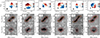 |
Fig. A.1. Examples of the kinematic data and models for our sample across our M* range. We show their velocity field (top), major-axis PV (middle), and minor-axis PV (bottom). The top panels also show the centre (white cross), kinematic major axis (dashed black line), and PSF (grey ellipse). In the PV plots, data are shown in a grey background and black contours (grey for negative values), and the best-fitting 3DBarolo model is in red. Line-of-sight velocities are shown in yellow. Contours are at −2, 2, 2nσr.m.s.. |
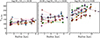 |
Fig. A.2. Hα rotation curves of our galaxy sample, derived with 3DBarolo. Galaxies are divided into three bins according to their stellar mass. All our rotation curves and velocity dispersion measurements are available upon request. |
In Sect. 4.1, we present our z = 0.9 TFR and FR. Upon close inspection of the data, we notice that there is a trend with Vf/σmed, such that at fixed M* galaxies with higher Vf/σmed have also a higher Vf and j*. This is shown in Fig. A.3. Similar trends for the FR at z ∼ 1 − 3 have been reported before (e.g. Burkert et al. 2016; Harrison et al. 2017; Bouché et al. 2021), and we have now confirmed them with accurate kinematic modelling that self-consistently derives the rotation and velocity dispersions.
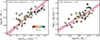 |
Fig. A.3. Dependency of the z = 0.9 TFR and FR on Vf/σmed. The solid pink curves and shaded bands represent our best-fit relations and their 1 σ confidence bands, respectively. |
Appendix B: Calibrating our measurement technique with galaxies at z ∼ 0
Given our methodology presented in Sect. 3, it is particularly crucial to ensure that we can recover the characteristic velocities at the flat part of our rotation curves (either Vcirc, f or Vf). To ensure that our methods are reliable, we tested and calibrated them on a sample of nearby disc galaxies (which have a similar Sérsic distribution to our sample) using detailed, accurate measurements of Vf and j* based on high-resolution rotation curves and NIR photometry. Specifically, we used the SPARC compilation (Lelli et al. 2016), which is also the sample used by Marasco et al. (2025) to derive the z = 0 TFR and FR we compare against in Sect. 4.2. The SPARC galaxies have Vf and j* measurements from Lelli et al. (2016), Posti et al. (2018) and Mancera Piña et al. (2021a), respectively, which were derived from the data without the use of any functional forms.
We have corroborated that our approach is robust as follows. First, we cut the SPARC rotation curves so they do not extend beyond 4 times their effective radius (derived from Sérsic fits to the SPARC surface brightness profiles). Second, we downsample the rotation curves by linear interpolation to extract rotational speeds at only four radii (the results remain unchanged when performed at three or five radii). These two steps ensure that the downsampled rotation curves resemble those from the z = 0.9 Hα data. Next, we fit the rotation curves with arctan profiles as in Sect. 3.
From empirical tests, we find that the best way to retrieve the characteristic flat velocity from the low-resolution data is to evaluate the best-fitting arctan model at R = 2 Reff for galaxies with Va > 100 km/s and R = 3 Reff for galaxies with Va < 100 km/s. As shown in the left panel of Fig. B.1, this results in an excellent agreement with the high-resolution measurements, with only a negligible offset. Similarly, we measure j* sampling Eq. 6 as described in the main text, and compare our values against the high-resolution estimates (right panel in Fig. B.1). Once again, there is an excellent agreement, with low residuals and scatter. From this discussion, we conclude that our methodology for deriving the characteristic flat velocity and j* is robust. We have also double-checked that the z = 0 TFR and FR re-derived with this technique have slopes and intercepts compatible with those inferred by Marasco et al. (2025).
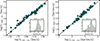 |
Fig. B.1. Calibration of our Vf (left) and j* (right) estimates. The figure compares the measurements at z = 0 obtained from high-resolution kinematics with those from downsampled rotation curves, which have a low spatial sampling similar to the z = 0.9 Hα data. The agreement is excellent, as highlighted by the residuals shown in the insets. |
Appendix C: Abundance-matching expectations
As discussed in the main text, the fM values found at z = 0.9 (but also at z = 0) are different from those expected from Moster et al. (2010) based on abundance-matching techniques. To visualise the level of this disagreement, in Fig. C.1 we compare the observed TFRs with those implied by the fM − M* relations from Moster et al. (2010), after assuming the same fV as in Sect. 5.1, i.e. solving Eq. 15 for the abundance-matching TFRs.
At low z (note that here we have assumed Vcirc, f = Vf) we can see discrepancies previously known in the literature, namely some dwarfs with lower M* than expected (the ‘baryon deficient dwarfs’ from Mancera Piña et al. 2025, see also Forbes & Gannon 2024), and some massive spirals with higher M* than predicted by abundance matching (e.g. Posti et al. 2019a; Marasco et al. 2020; Di Teodoro et al. 2023; Mancera Piña et al. 2022). Our observations show that the discrepancies with abundance matching become much more dramatic at z = 0.9, with the abundance-matching TFR being about 0.7 dex too low in log(M*) or 0.25 dex in log(Vf), and with a curvature not evident in the data. Alternatively, setting fV = 0.8 would make the abundance-matching expectations consistent with the data, but it is unlikely that such a low value is valid for our M* range (McGaugh 2012).
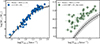 |
Fig. C.1. Observed TFRs against the predictions from abundance matching, after assuming the fV discussed in the main text. Note the differences in the axes span. |
Appendix D: Sample and main physical parameters
Main parameters of our galaxy sample.
All Tables
Best-fitting parameters (α, β, ϵ⊥) and vertical RMS scatter (σM* for the TFR and σj* for the FR) of our z = 0.9 TFR and FR.
All Figures
|
Fig. 1. Top left: The SFMS defined by our high-z galaxies, colour-coded by their redshift. The reference SFMS from Leja et al. (2022) is shown. Star formation rates come from our SED fitting. Top right: Rotation to dispersion ratio for our galaxy sample. Bottom left: Sérsic index as a function of M*. The inset shows the cumulative distribution of the Sérsic indices. Bottom right: Stellar mass-size relation. Our galaxies (green markers) are contrasted against (1) the individual measurements from Martorano et al. (2024) at 0.8 ≤ z ≤ 1 (blue markers) and their 1 and 2 σ ranges (blue bands), and (2) the relation from van der Wel et al. (2014) at z = 0.75 after applying approximate corrections to account for the sizes differences in optical vs. NIR bands. |
| In the text | |
|
Fig. 2. Our z = 0.9 scaling laws. The TFR is shown on the left, and the FR on the right. Our measurements are shown with the green markers, while the best-fit relations and their 1σ confidence bands are shown as solid pink curves and bands, respectively. For comparison, we show the z = 0 TFR and FR from Marasco et al. (2025). |
| In the text | |
|
Fig. 3. Posterior distributions of the best-fitting TFR and FR. The distributions of low- and high-z disc galaxies are shown in blue (from Marasco et al. 2025) and pink (this work), respectively. The contours encompass the 0.393, 0.865, and 0.989 percentiles, corresponding to 1, 2, and 3σ in 2D distributions. |
| In the text | |
|
Fig. 4. Drivers of the evolution in our scaling relations. The top panels compare how the local TFR and FR (blue curves) would evolve (orange curves) if the only changes are the z evolution of the Hubble parameter and the density contrast, against our high-z data (green markers) and best fits (pink curves). The results imply an evolution of |
| In the text | |
|
Fig. 5. Comparison between our inferred fM − M* (top) and Mvir − M* (bottom) relations and an idealised toy model of mass assembly. The model considers a population of galaxies (blue circles) lying in the z = 0 relations (blue curves), which are then traced back to z = 0.9 (squares), assuming theoretical stellar and halo mass growths. Galaxy downsizing and halo growth histories yield z = 0.9 relations (squares) with slopes different from those observed at z = 0 (solid pink curves). The only way to reconcile the stellar mass growth of galaxies with our inferred relations at z = 0.9 is if low-mass haloes grew more than high-mass haloes since z = 0.9, contrary to CDM expectations. This suggests that the galaxies populating our z = 0.9 relations do not follow this toy model and are unlikely to be the progenitors of the z = 0 population. |
| In the text | |
|
Fig. A.1. Examples of the kinematic data and models for our sample across our M* range. We show their velocity field (top), major-axis PV (middle), and minor-axis PV (bottom). The top panels also show the centre (white cross), kinematic major axis (dashed black line), and PSF (grey ellipse). In the PV plots, data are shown in a grey background and black contours (grey for negative values), and the best-fitting 3DBarolo model is in red. Line-of-sight velocities are shown in yellow. Contours are at −2, 2, 2nσr.m.s.. |
| In the text | |
|
Fig. A.2. Hα rotation curves of our galaxy sample, derived with 3DBarolo. Galaxies are divided into three bins according to their stellar mass. All our rotation curves and velocity dispersion measurements are available upon request. |
| In the text | |
|
Fig. A.3. Dependency of the z = 0.9 TFR and FR on Vf/σmed. The solid pink curves and shaded bands represent our best-fit relations and their 1 σ confidence bands, respectively. |
| In the text | |
|
Fig. B.1. Calibration of our Vf (left) and j* (right) estimates. The figure compares the measurements at z = 0 obtained from high-resolution kinematics with those from downsampled rotation curves, which have a low spatial sampling similar to the z = 0.9 Hα data. The agreement is excellent, as highlighted by the residuals shown in the insets. |
| In the text | |
|
Fig. C.1. Observed TFRs against the predictions from abundance matching, after assuming the fV discussed in the main text. Note the differences in the axes span. |
| In the text | |
Current usage metrics show cumulative count of Article Views (full-text article views including HTML views, PDF and ePub downloads, according to the available data) and Abstracts Views on Vision4Press platform.
Data correspond to usage on the plateform after 2015. The current usage metrics is available 48-96 hours after online publication and is updated daily on week days.
Initial download of the metrics may take a while.