| Issue |
A&A
Volume 705, January 2026
|
|
|---|---|---|
| Article Number | A40 | |
| Number of page(s) | 16 | |
| Section | Stellar atmospheres | |
| DOI | https://doi.org/10.1051/0004-6361/202557581 | |
| Published online | 07 January 2026 | |
Spectropolarimetric characterisation of exoplanet host stars in preparation of the Ariel mission
II. The magnetised wind environment of TOI-1860, DS Tuc A, and HD 63433
1
Leiden Observatory, Leiden University,
PO Box 9513,
2300
RA
Leiden,
The Netherlands
2
Institut de Recherche en Astrophysique et Planétologie, Université de Toulouse, CNRS,
IRAP/UMR 5277, 14 avenue Edouard Belin,
31400
Toulouse,
France
3
Centre for Planetary Habitability (PHAB), Department for Geosciences, University of Oslo,
Oslo,
Norway
4
INAF – Osservatorio Astrofisico di Arcetri,
Largo E. Fermi 5,
50125
Firenze,
Italy
5
SRON, Netherlands Institute for Space Research,
Niels Bohrweg 4,
2333
CA,
Leiden,
The Netherlands
6
Department of Physics and Astronomy, University College London,
Gower Street,
WC1E 6BT
London,
UK
7
Science Engagement and Oversight Office, Directorate of Science, European Space Research and Technology Centre (ESA/ESTEC),
Keplerlaan 1,
2201
AZ,
Noordwijk,
The Netherlands
8
Laboratoire Univers et Particules de Montpellier, Université de Montpellier, CNRS,
34095
Montpellier,
France
9
University of Vienna, Department of Astrophysics,
Türkenschanzstrasse 17,
1180
Vienna,
Austria
10
INAF – Osservatorio Astronomico di Palermo,
Piazza del Parlamento 1,
90134
Palermo,
Italy
★ Corresponding author: This email address is being protected from spambots. You need JavaScript enabled to view it.
Received:
7
October
2025
Accepted:
28
November
2025
Abstract
Aims. We update the status of the spectropolarimetric campaign dedicated to characterise the magnetic field properties of a sample of known exoplanet-hosting stars included in the current target list of the Ariel mission. The main aims are to inform observing strategies and subsequent analysis of the data of the Ariel mission, and to provide background information on the magnetic properties of the target and their variability on timescales of at least a few years.
Methods. We analysed spectropolarimetric data collected for 15 G-M type stars with Neo-Narval, HARPSpol, and SPIRou to assess the detectability of the large-scale magnetic field. For three stars we reconstructed the magnetic field topology and its temporal evolution via Zeeman-Doppler imaging (ZDI). Such reconstructions were then used to perform three-dimensional magnetohydrodynamical simulations of the stellar wind and environment impinging on the hosted exoplanets.
Results. We detected the magnetic field of six stars. Of these, we performed ZDI reconstructions for the first time of TOI-1860 and DS Tuc A, and for the second time of HD 63433, providing temporal information of its large-scale magnetic field. Consistently with previous results on young (~50–100 Myr) solar-like stars, the large-scale magnetic field is moderately strong (30–60 G on average) and complex, with a significant fraction of magnetic energy in the toroidal component and high-order poloidal components. From the simulations of the stellar wind, we found the orbit of TOI-1860 b to be almost completely sub-Alfvénic, the orbits of DS Tuc A b and HD 63433 d to be trans-Alfvénic, and the orbits of HD 63433 b and c to be super-Alfvénic. We obtained marginal detections of the magnetic field for TOI-836 and TOI-2076, and detections for TOI-1136, but the number of observations is not sufficient for magnetic mapping.
Conclusions. A magnetic star-planet connection can occur for most of TOI-1860 b’s orbit. This can happen more sporadically for DS Tuc A b and HD 63433 c given the lower fraction of their orbit in the sub-Alfvénic regime. The orbit of HD 63433 c is nevertheless more sub-Alfvénic than previously simulated owing to the temporal evolution of the stellar magnetic field. For HD 63433 b and c, we expect the formation of a bow shock between the stellar wind and the planet despite the evolution of the stellar magnetic field.
Key words: techniques: polarimetric / stars: activity / stars: magnetic field
© The Authors 2026
 Open Access article, published by EDP Sciences, under the terms of the Creative Commons Attribution License (https://creativecommons.org/licenses/by/4.0), which permits unrestricted use, distribution, and reproduction in any medium, provided the original work is properly cited.
This article is published in open access under the Subscribe to Open model. This email address is being protected from spambots. You need JavaScript enabled to view it. to support open access publication.
1 Introduction
Ariel is a medium-class (M4) science mission of the European Space Agency planned to be launched in 2029 (Tinetti et al. 2018, 2022). The aim of Ariel is to perform a comprehensive survey of the chemical composition and structure of exoplanetary atmospheres, in order to understand exoplanets’ bulk composition and how planetary systems form and evolve. The mission will target about a thousand transiting planets orbiting different types of host stars, from early A type to late M (Zingales et al. 2018; Edwards et al. 2019; Edwards & Tinetti 2022)1.
To perform an informed target selection and optimise the observing strategy of Ariel, it is important to characterise exoplanet-hosting stars in a homogeneous manner (Danielski et al. 2022; Magrini et al. 2022). This is also crucial to prevent a biased interpretation of the planetary atmosphere and chemistry. Stellar magnetic activity is a known source of uncertainty in differential spectroscopy analyses (Pont et al. 2007, 2013), because it can alter the stellar spectrum on the timescale of the transit (Spina et al. 2020). Magnetically induced inhomogeneities on stellar surfaces hinder the precise measurement of both the planetary radius and mass, therefore affecting the atmospheric scale height estimate and the subsequent retrieval (Oshagh et al. 2013; Changeat et al. 2020; Di Maio et al. 2023). Depending on the coverage and global configuration of these magnetic inhomogeneities, ambiguous atomic and molecular absorption and emission features can occur (e.g. Rackham et al. 2018, 2019; Salz et al. 2018; Genest et al. 2022). Moreover, the magnetic field of stars governs the amount of short-wavelength radiation (such as extreme ultraviolet and X-rays Güdel 2004; Reiners et al. 2022) and stellar wind impinging on planets (e.g. Vidotto et al. 2015; Garraffo et al. 2016; Alvarado-Gómez et al. 2022), ultimately regulating photochemistry (e.g. Locci et al. 2022, 2024) and the erosion of planetary atmospheres (e.g. Lammer et al. 2003; Lanza 2013; McCann et al. 2019; Carolan et al. 2021a; Hazra et al. 2020; Presa et al. 2024; Van Looveren et al. 2025).
In this paper, we update the status of the spectropolarimetric survey aimed at characterising the stellar magnetic field properties and surrounding environment of a representative sample of stars in the current list of potential Ariel targets (Edwards et al. 2019; Edwards & Tinetti 2022). The work of Bellotti et al. (2024) introduced such a survey and focussed on the solar-type star HD 63433. With the information on the stellar large-scale magnetic field at hand, stellar wind simulations have shown that young active stars could produce wind conditions that are harsher compared to the present solar neighbourhood (see Vidotto et al. 2012; Nicholson et al. 2016; Folsom et al. 2020; Vidotto et al. 2023, for a few examples). Being dictated by the stellar magnetic field, the environment varies over time in correlation with the stellar magnetic cycle (McComas 2003, Smith et al., in review) and the evolution of the star (e.g. Johnstone et al. 2021). As a result, the region of space in which specific magnetic star-planet interactions take place could be temporarily modified, altering both the nature and intensity of these interactions.
Our survey is divided into three steps (see also Bellotti et al. 2024): (1) a snapshot campaign to assess the detectability of the large-scale magnetic field and optimise further observations, (2) an observing campaign to reconstruct the topology of the surface’s stellar magnetic field, and (3) a long-term monitoring to constrain the evolution and variability of the field. The work presented in this paper addresses all of these steps for new targets with respect to Bellotti et al. (2024). We first describe the snapshot polarimetric observations aimed at determining which stars are suitable for spectropolarimetric follow-up. Then we present the first large-scale magnetic field reconstructions via Zeeman-Doppler imaging (ZDI; Semel 1989; Donati et al. 1997) for TOI-1860 and DS Tuc A. Finally, we provide a new ZDI reconstruction for HD 63433. The large-scale magnetic field topology of this star was previously reconstructed by Bellotti et al. (2024), and hence we analyse its temporal evolution over a timescale of a year.
This paper is structured as follows. In Sect. 2, we describe the target selection for this study and the spectropolarimetric observations and in Sect. 3 we analyse the detectability of the large-scale magnetic field. In Sect. 4, we focus on the reconstruction of the large-scale magnetic field of TOI-1860, DS Tuc A, and HD 63433 and in Sect. 5 we describe the magnetohydrodynamical simulations of the environment around these stars. We finally discuss our results and draw our conclusions in Sect. 6.
2 Observations
2.1 Target selection
The construction of the current Ariel target list is described in Edwards et al. (2019), Mugnai et al. (2020), and Edwards & Tinetti (2022). It contains 748 exoplanet systems whose host stars have a spectral type ranging from A (Teff ~ 10 000 K) to late M (Teff ~ 2600 K). Starting from this list, we applied a series of selection criteria to obtain a sample of stars whose properties are supposedly suitable for magnetometry. The stars should: (i) be bright enough in order to carry out observations with a reasonable exposure time and obtain a moderate signal-to-noise ratio (S/N), and (ii) exhibit a certain level of magnetic activity as quantified by specific proxies. The latter point would then translate into a potentially detectable large-scale magnetic field.
We applied the following quantitative selection criteria:
Stellar mass M* < 1.2 M⊙. The outer convective envelopes typical of these type of stars are known to produce persistent and intense magnetic fields via dynamo (e.g. Schrijver & Zwaan 2000).
Rotation period Prot < 30 d, equatorial velocity veq sin i > 2 km s−1, and chromospheric activity S-index > 0.2 (or
![Mathematical equation: $\[\log~ R_{\mathrm{HK}}^{\prime}>-4.8\]$](/articles/aa/full_html/2026/01/aa57581-25/aa57581-25-eq1.png) ). These selection limits, corresponding to fast rotation and high magnetic activity, translate into magnetic detection fractions larger than 70% according to the results of the Bcool snapshot survey (Marsden et al. 2014).
). These selection limits, corresponding to fast rotation and high magnetic activity, translate into magnetic detection fractions larger than 70% according to the results of the Bcool snapshot survey (Marsden et al. 2014).Magnitude in H or V band lower than 9.0. This threshold is applied to limit a polarimetric exposure to a maximum of approximately one hour for spectropolarimeters operating at optical or near-infrared wavelengths.
We applied conservative activity thresholds to search for the most active stars in the current list of Ariel targets. Although HD 63935 and HD 89345 have veq sin i < 2 km s−1, we kept them in our list because of their brightness. We also kept HD 260655 albeit its rotation period is 37.5 d because Lehmann et al. (2024) recently showed that slowly rotating (Prot ~ 100 d) M dwarfs are capable of generating strong magnetic fields. In general, our selection criteria include the mass dependency of the rotation-activity relation (e.g. Pizzolato et al. 2003), but indirectly, since other factors such as brightness dominate our shortlisting. Indeed, most of the M dwarfs in the Ariel Candidate Sample are too faint to be efficiently observed with spectropolarimetry, regardless of their rotation period or activity level. Finally, we did not select stars that have a spectropolarimetric characterisation already, such as GJ 436 (Bellotti et al. 2023a; Vidotto et al. 2023) and AU Mic (Klein et al. 2021; Donati et al. 2023) for instance.
The stellar sample analysed in this work contains 15 objects and its properties are listed in Table 1. The fraction of low-mass, highly-to-moderately active stars in the Ariel Candidate Sample that are shortlisted with our selection criteria excluding the magnitude criterion is ~30%. Our 15 stars are therefore representative of the bright end of this specific parameter space. We note that for ![Mathematical equation: $\[\log~ R_{\mathrm{HK}}^{\prime}\]$](/articles/aa/full_html/2026/01/aa57581-25/aa57581-25-eq2.png) we are currently using literature values, but that in the future publications we will use homogeneous data that are currently being prepared by Wizani et al, in prep. We also note that the list of targets for Ariel is being optimised over time, hence some of the targets selected for this spectropolarimetric campaign may have been removed from the mission candidate sample, but they remain interesting targets (e.g. for other follow-up efforts than Ariel).
we are currently using literature values, but that in the future publications we will use homogeneous data that are currently being prepared by Wizani et al, in prep. We also note that the list of targets for Ariel is being optimised over time, hence some of the targets selected for this spectropolarimetric campaign may have been removed from the mission candidate sample, but they remain interesting targets (e.g. for other follow-up efforts than Ariel).
Properties of the selected stars.
2.2 Instruments
We analysed spectropolarimetric observations collected with Neo-Narval, HARPSpol, and SPIRou. The journal of the observations can be found in Table B.1, excluding the 2023 observations of HD 63433 published in Bellotti et al. (2024).
Neo-Narval2 is the upgraded version of Narval (López Ariste et al. 2022) mounted on the 2 m Télescope Bernard Lyot (TBL) at the Pic du Midi Observatory in France (Donati 2003). The upgrade occurred in 2019, and kept the main performances of Narval: a spectral coverage from 380 to 1050 nm, and a median spectral resolving power of ~65 000 after data reduction (López Ariste et al. 2022).
HARPSpol3 (Snik et al. 2011; Piskunov et al. 2011) is the spectropolarimeter for the HARPS spectrograph (Mayor et al. 2003) mounted at the Cassegrain focus of the ESO 3.6 m telescope at La Silla observatory, Chile. HARPSpol observations cover the wavelength range between 380 and 691 nm with a 8 nm gap at 529 nm separating the red and blue detectors. The resolving power is R ~ 110 000. The data reduction was carried out with the PyReduce package4 (Piskunov et al. 2021), the updated implementation in python of the versatile REDUCE package (Piskunov & Valenti 2002). The reduction with PyReduce is run with a series of standard steps, similar to REDUCE as described by Rusomarov et al. (2013). For more information on the steps applied to our observations see Bellotti et al. (2024).
The SpectroPolarimètre InfraRouge (SPIRou5) is the near-infrared spectropolarimeter mounted at Cassegrain focus on the 3.6 m CFHT atop Maunakea, Hawaii (Donati et al. 2020). The instrument allows linear and circular polarisation observations at a spectral resolving power of R ~ 70 000 for a wavelength coverage between 960 to 2500 nm (YJHK bands). Optimal extraction of SPIRou spectra was carried out with A PipelinE to Reduce Observations (APERO v0.6.132), a fully automatic reduction package installed at CFHT (Cook et al. 2022).
Our observations were carried out in circular polarisation mode. The output consists of unpolarised (Stokes I), circularly polarised (Stokes V) and null (Stokes N) high-resolution spectra. The Stokes N spectrum is practical to check the presence of spurious polarisation signatures or data reduction issues (see Donati et al. 1997; Bagnulo et al. 2009; Tessore et al. 2017, for more details).
3 Magnetic field detectability
3.1 Least-squares deconvolution
For the first part of our campaign dedicated to the detectability of the large-scale magnetic field, we requested a handful of observations per star at separated days throughout the observing semester. We applied least-squares deconvolution (LSD; Donati et al. 1997; Kochukhov et al. 2010) to the collected unpolarised, circularly polarised and null spectra. We used the pylsd python code6 which is part of the specpolflow package (Folsom et al. 2025) to deconvolve the spectra with a synthetic atomic line list. Together with wavelength, a line list typically contains the associated atomic number, depth, excitation potential, and effective Landé factor (indicated as geff), which encapsulates the sensitivity to Zeeman effect. The deconvolution results in an single, high-signal-to-noise ratio (S/N) kernel (for Stokes I, V, and N) summarising the properties of hundreds or thousands of spectral lines.
We generated synthetic line lists via the Vienna Atomic Line Database7 (VALD, Ryabchikova et al. 2015), selecting models whose effective temperature and surface gravity are close to the values reported in the Ariel stellar group catalogue for each target. For observations at optical wavelengths with Neo-Narval and HARPSpol, we chose atomic lines between 350 and 1097 nm, with known geff, and whose depth relative to the continuum is larger than 40% (following Moutou et al. 2007). We adopted an LSD normalisation wavelength of 700 nm and a normalisation geff of 1.2. For observations at near-infrared wavelengths with SPIRou, we selected atomic lines between 950 and 2600 nm, with known geff, and with a relative depth larger than 3% (see e.g. Bellotti et al. 2023b). In this case we adopted a normalisation wavelength of 1700 nm and a normalisation Landé factor of 1.2.
The properties of the synthetic line lists used in this work are summarised in Table 2, in which we also report the total number of spectropolarimetric observations. To quantify whether a circularly polarised Zeeman signature is detected, and thus the large-scale magnetic field, we computed the false-alarm probability (FAP; see Donati et al. 1997, for more details). A successful detection corresponds to FAP < 10−4, and a marginal detection to FAP = 10−2 − 10−4. The same metric is applied to Stokes N in order to check for spurious polarisation signatures. The results are listed in Table B.1.
Zeeman signatures in circular polarisation are detected for TOI-1136, TOI-1860, and DS Tuc A, as well as for the newest observations of HD 63433. As a result, these stars are amenable to magnetic field characterisation. For TOI-836 we obtained one marginal detection and for TOI-2076 we obtained two while the remaining four observations are non-detections. While for TOI-836, TOI-1136, and TOI-2076 we require additional observations for producing a ZDI map, for TOI-1860, HD 63433, and DS Tuc A we collected a number of observations that sample various longitudes and are sufficient for the ZDI reconstruction (see Sect. 4).
We did not detect circularly polarised Zeeman signatures in eight stars over multiple snapshot observations. This is not completely surprising as exoplanets are more easily detected around magnetically inactive stars, that is with a weak largescale magnetic field. Another possibility is that the large-scale configuration of these stars is such that the magnetic polarity cancellation is substantial, although distributing multiple observations across the semester should allow for some detections owing to stellar rotation and magnetic field variability. This aspect makes the substantial polarity cancellation scenario less likely. The number of non-detections of our stars are overall in agreement with the statistics of the BCool campaign (Marsden et al. 2014), for which a moderate fraction of the large-scale magnetic field of stars with surface temperature between 5250 K and 6000 K (that is, spectral types G5 to G0) is not detected. This is also noted considering the stellar rotation period, since most of our non-detections are for slowly rotating stars with Prot > 20 d.
Properties of the synthetic line lists.
3.2 Longitudinal magnetic field
The longitudinal magnetic field is the net, line-of-sight-projected component of the large-scale magnetic field (e.g. Donati et al. 1997). We used the general formula as in Cotton et al. (2019),
![Mathematical equation: $\[\mathrm{B}_{\mathrm{l}}=\frac{\mathrm{h}}{\mu_{\mathrm{B}} \lambda_0 \mathrm{g}_{\mathrm{eff}}} \frac{\int \mathrm{vV}(\mathrm{v}) \mathrm{dv}}{\int\left(\mathrm{I}_{\mathrm{c}}-\mathrm{I}(\mathrm{v})\right) \mathrm{dv}},\]$](/articles/aa/full_html/2026/01/aa57581-25/aa57581-25-eq4.png) (1)
(1)
where λ0 and geff are the normalisation wavelength and Landé factor of the LSD profiles, Ic is the continuum level, v is the radial velocity associated to a point in the spectral line profile in the star’s rest frame, h is the Planck’s constant and μB is the Bohr magneton. To express it as in Rees & Semel (1979) and Donati et al. (1997), one can use hc/μB = 0.0214 Tm, where c is the speed of light in m s−1.
We computed the longitudinal magnetic field (Bl) for TOI-836, TOI-1136, TOI-1860, TOI-2076, HD 63433, and DS Tuc A using the continuum-normalised Stokes profiles. In practice, we fitted a linear model to the region outside the Stokes I LSD profile, to include residuals of continuum normalisation at the level of the spectra, and we re-scaled the Stokes V LSD profiles by the same fit. For TOI-1136 and TOI-2076, we used only the observations in which Stokes N detection is at most marginal. For the stars without detections, we computed 3σ upper limits. The results are given in Table B.1.
For TOI-1136, the integral range was set to ±15 km s−1. For the two observations when Stokes V was marginally and completely detected and Stokes N showed only a marginal detection (18 and 19 March 2024), we obtained 25 ± 44 G and 131 ± 60 G, where the error bar indicates the 1σ formal uncertainty. We caution that the presence of a marginal detection in Stokes N can alter the polarisation signature in Stokes V, ultimately affecting the value of Bℓ. For TOI-2076 we integrated Eq. (1) between ±20 km s−1 and obtained −75 ± 17 G and 69 ± 34 G.
For TOI-1860, the integral range was set to ±25 km s−1. For the observations in 2024 with a detection, we found values between −5 G and 19 G and for the 2025 observations we found values between −21 G and 20 G. For DS Tuc A, we used a range of ±35 km s−1 and obtained values between −36 G and −4 G, with an average of −19 G. For HD 63433, we applied Eq. (1) between ±20 km s−1 from the line centre at −15.9 km s−1. We found values between −6 G and 5 G, with an average of −1.0 G, similar to the measurements on the 2023 data (Bellotti et al. 2024).
Properties of the large-scale magnetic field and wind of the studied stars.
4 Large-scale magnetic field reconstruction
The second and third parts of our spectropolarimetric campaign are dedicated to reconstructing the stellar large-scale magnetic field for the first time or across different epochs. So far, we have performed enough monitoring to reconstruct a ZDI map for TOI-1860, DS Tuc A, and HD 63433. For TOI-1860, we only used the June and July 2025 data set, since the August 2025 data yielded non-detections and the 2024 data set did not have enough observations. The ZDI algorithm inverts a time series of Stokes V LSD profiles into a magnetic field map, by iteratively synthesising and adjusting model Stokes V profiles, until a maximum-entropy solution at a fixed reduced χ2 is achieved (for more information, see Skilling & Bryan 1984; Donati & Brown 1997; Folsom et al. 2018). The field is formally described as the sum of a poloidal and toroidal component, which are both expressed via spherical harmonic decomposition (Donati et al. 2006; Lehmann & Donati 2022). The odd and even spherical harmonics modes are weighted equally in the reconstruction. We employed the zdipy code described in Folsom et al. (2018).
We adopted the weak-field approximation because local field strengths are lower than 160 G for our targets (see Table 3), that is, within the range of applicability of the approximation (typically less 1 kG Kochukhov et al. 2010). We note that magnetic field strengths at unresolved spatial scales are most likely larger than 1 kG as corroborated by Zeeman broadening and intensification measurements (see Kochukhov et al. 2020; Hahlin et al. 2023, for some recent results). Assuming weak-field approximation, Stokes V is proportional to the derivative of Stokes I with respect to wavelength (e.g. Landi Degl’Innocenti 1992). The unpolarised line profiles in each cell of the stellar grid are modelled with a Voigt kernel, parametrised by the line depth (d), Gaussian width (wG), and Lorentzian width (wL). The optimal values of these three parameters are obtained with a ![Mathematical equation: $\[\chi_{r}^{2}\]$](/articles/aa/full_html/2026/01/aa57581-25/aa57581-25-eq8.png) minimisation between the median of the observed Stokes I LSD profiles and its model over a grid of (d, wG, wL) values. We provide the optimal values for each star below.
minimisation between the median of the observed Stokes I LSD profiles and its model over a grid of (d, wG, wL) values. We provide the optimal values for each star below.
The stellar input parameters of ZDI are the rotation period Prot, the projected equatorial velocity veq sin(i), and the inclination i (that is, the viewing angle). Furthermore, the ZDIPY code includes surface shear as a function of colatitude (θ) expressed in the form
![Mathematical equation: $\[\Omega(\theta)=\Omega_{\mathrm{eq}}-\mathrm{d} \Omega ~\sin ^2(\theta),\]$](/articles/aa/full_html/2026/01/aa57581-25/aa57581-25-eq9.png) (2)
(2)
where Ωeq = 2π/Prot is the rotational frequency at equator and dΩ is the differential rotation rate in rad d−1. The variable dΩ is also an input parameter of ZDI.
The input veq sin(i) used for TOI-1860, DS Tuc A, and HD 63433 is listed in Table 1. The stellar inclination was estimated comparing the stellar radius provided in the stellar working group catalogue with the projected radius R sin i = Protveq sin i/50.59, where R sin(i) is measured in solar radii, Prot in d, and veq sin i in km s−1. We estimated i ≃ 90° for DS Tuc A and TOI-1860, so we adopted a value of i = 80° in ZDI to prevent mirroring effects between the northern and southern hemispheres that a value of 90° would incur. For HD 63433, we used i = 70° as constrained by Mann et al. (2020).
For the latitudinal differential rotation, we performed the parameter optimisation outlined in Donati et al. (2000) and Petit et al. (2002). We generated a grid of (Prot, dΩ) pairs, reconstructed a ZDI map for each of the pairs, and searched for the values that minimised the ![Mathematical equation: $\[\chi_{r}^{2}\]$](/articles/aa/full_html/2026/01/aa57581-25/aa57581-25-eq10.png) distribution between observations and synthetic LSD profiles, at a fixed entropy level. The best parameters are measured by fitting a 2D paraboloid to the
distribution between observations and synthetic LSD profiles, at a fixed entropy level. The best parameters are measured by fitting a 2D paraboloid to the ![Mathematical equation: $\[\chi_{r}^{2}\]$](/articles/aa/full_html/2026/01/aa57581-25/aa57581-25-eq11.png) distribution, and the error bars are obtained from a variation of
distribution, and the error bars are obtained from a variation of ![Mathematical equation: $\[\Delta \chi_{r}^{2} = 1\]$](/articles/aa/full_html/2026/01/aa57581-25/aa57581-25-eq12.png) away from the minimum (Press et al. 1992; Petit et al. 2002). If no differential rotation is constraint, we assumed solid body rotation with Prot from Table 1.
away from the minimum (Press et al. 1992; Petit et al. 2002). If no differential rotation is constraint, we assumed solid body rotation with Prot from Table 1.
In general, a faster rotation (that is, larger veq sin(i)) translates into a decreased polarity cancellation because the Zeeman signatures are more separated in radial velocity space (see Hussain et al. 2009, for example). For this reason, we set the maximum degree of spherical harmonic coefficients ℓmax to 10 for every ZDI reconstruction. We note that a lower value could have been used, since most of the magnetic energy is stored in the ℓ < 6 degrees. Finally, we fixed the V-band limb darkening coefficient to 0.6964 (Claret & Bloemen 2011).
For each of the three stars, the observations were phased with the following ephemeris
![Mathematical equation: $\[\mathrm{HJD}=\mathrm{HJD}_0+\mathrm{P}_{\mathrm{rot}} \mathrm{n}_{\mathrm{cyc}},\]$](/articles/aa/full_html/2026/01/aa57581-25/aa57581-25-eq13.png) (3)
(3)
where Prot is the stellar rotation period and ncyc is the rotation cycle. The reference heliocentric Julian date HJD0 is the first observation or the median observation, depending on whether solid body rotation or differential rotation was assumed.
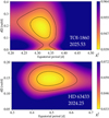 |
Fig. 1 Joint search of differential rotation and equatorial rotation period for TOI-1860 (top) and HD 63433 (bottom). The panels illustrate the |
![Mathematical equation: $\[\chi_{r}^{2}\]$](/articles/aa/full_html/2026/01/aa57581-25/aa57581-25-eq14.png)
4.1 TOI-1860
As reported in Table 1, TOI-1860 has a rotation period of 4.43 d and veq sin(i) = 10.4 km s−1 (Giacalone et al. 2022). The optimised Voigt kernel parameters are d = 1.95, wG = 1.12 km s−1, and wL = 3.0 km s−1 and the assumed inclination is 80°. Our ten Neo-Narval observations span 23 d (or 5.2 rotational cycles), so a surface shear would have had the time to distort the LSD profiles sufficiently to be detected. The result of the differential rotation search is shown in Fig. 1. The analysis yielded Prot = 4.315 ± 0.035 d and dΩ = 0.189 ± 0.089 rad d−1, which implies a rotation period at the pole of Prot = 4.959 ± 0.351 d (see Eq. (2)) and an equator-pole lap time of 33 d. The value of dΩ is consistent with typical latitudinal differential rotation rates of young solar-like stars (see Bellotti et al. 2025b, for a recent example). Although the ![Mathematical equation: $\[\chi_{\mathrm{r}}^{2}\]$](/articles/aa/full_html/2026/01/aa57581-25/aa57581-25-eq15.png) landscape features a minimum, the lower boundary of the grid features a decrease in
landscape features a minimum, the lower boundary of the grid features a decrease in ![Mathematical equation: $\[\chi_{\mathrm{r}}^{2}\]$](/articles/aa/full_html/2026/01/aa57581-25/aa57581-25-eq16.png) making the overall landscape shape irregular. This is reflected in a large error bar of the differential rotation rate. Moreover, Petit et al. (2002) showed that when estimating dΩ with fewer phases than about 15, rotational phase gaps tend to generate biases that are not included in the statistical error bar.
making the overall landscape shape irregular. This is reflected in a large error bar of the differential rotation rate. Moreover, Petit et al. (2002) showed that when estimating dΩ with fewer phases than about 15, rotational phase gaps tend to generate biases that are not included in the statistical error bar.
The model Stokes V profiles were fit down to ![Mathematical equation: $\[\chi_{\mathrm{r}}^{2}\]$](/articles/aa/full_html/2026/01/aa57581-25/aa57581-25-eq17.png) = 0.98 (see Fig. A.1), from an initial value of 2.05 which corresponds to a featureless magnetic map. The target
= 0.98 (see Fig. A.1), from an initial value of 2.05 which corresponds to a featureless magnetic map. The target ![Mathematical equation: $\[\chi_{r}^{2}\]$](/articles/aa/full_html/2026/01/aa57581-25/aa57581-25-eq18.png) is determined by running ZDI over a grid of
is determined by running ZDI over a grid of ![Mathematical equation: $\[\chi_{r}^{2}\]$](/articles/aa/full_html/2026/01/aa57581-25/aa57581-25-eq19.png) values with all other parameters fixed, each time recording the entropy at convergence, and by measuring the maximum of the change rate in the entropy (see Alvarado-Gómez et al. 2015, for more details).
values with all other parameters fixed, each time recording the entropy at convergence, and by measuring the maximum of the change rate in the entropy (see Alvarado-Gómez et al. 2015, for more details).
The ZDI magnetic map is illustrated in Fig. 2 and its properties are listed in Table 3. The unsigned, mean magnetic field strength is Bmean = 37 G, and the topology is predominantly toroidal, as the corresponding component accounts for 72% of the total magnetic energy. Of the poloidal component, the dipolar, quadrupolar, and octupolar modes store 28%, 13%, and 26% of the energy. The large-scale toroidal component is mostly axisymmetric (98%) while the poloidal component is non-axisymmetric (11%).
4.2 DS Tuc A
For DS Tuc A, the optimal Voigt kernel parameters are: d = 0.52, wG = 1.75 km s−1, and wL = 4.0 km s−1. We set the rotation period to 2.85 d, the veq sin(i) to 17.8 km s−1 (Newton et al. 2019), and the inclination to 80°. The search for latitudinal differential rotation was inconclusive in this case, so we assumed solid body rotation.
The model Stokes V profiles were fit down to ![Mathematical equation: $\[\chi_{\mathrm{r}}^{2}\]$](/articles/aa/full_html/2026/01/aa57581-25/aa57581-25-eq20.png) = 1.6 (see Fig. A.1), from an initial value of 7.2. The target
= 1.6 (see Fig. A.1), from an initial value of 7.2. The target ![Mathematical equation: $\[\chi_{r}^{2}\]$](/articles/aa/full_html/2026/01/aa57581-25/aa57581-25-eq21.png) of 1.6 is most likely due to unconstrained differential rotation and slightly underestimated error bars, as the actual noise in the profile looks larger than the uncertainties in some instances. The ZDI magnetic map is illustrated in Fig. 2 and its properties are listed in Table 3. The unsigned, mean magnetic field strength is Bmean = 64 G, and the topology is predominantly poloidal (64%), with the dipolar, quadrupolar, and octupolar modes accounting for 67%, 12%, and 9% of the energy. The large-scale topology is also mostly axisymmetric, with 66% of the energy in the corresponding modes.
of 1.6 is most likely due to unconstrained differential rotation and slightly underestimated error bars, as the actual noise in the profile looks larger than the uncertainties in some instances. The ZDI magnetic map is illustrated in Fig. 2 and its properties are listed in Table 3. The unsigned, mean magnetic field strength is Bmean = 64 G, and the topology is predominantly poloidal (64%), with the dipolar, quadrupolar, and octupolar modes accounting for 67%, 12%, and 9% of the energy. The large-scale topology is also mostly axisymmetric, with 66% of the energy in the corresponding modes.
4.3 HD 63433
For HD 63433, the optimised Voigt kernel parameters are: d = 1.8, wG = 1.1 km s−1, and wL = 2.6 km s−1. The stellar inclination was fixed to 70° and the rotational velocity to 7.3 km s−1 (similar to Bellotti et al. 2024). Our nine Neo-Narval observations in 2024 span 28 d (or 4.3 rotational cycles), and the differential rotation search yielded a minimum at Prot = 6.489 ± 0.075 d and dΩ = 0.147 ± 0.023 rad d−1. In a similar manner to the dΩ result of TOI-1860, the gap in the rotational phases may be introducing biases. The latitudinal differential rotation translates into a rotation period at the pole of 7.650 ± 0.238 d and an equator-pole lap time of 43 d. The range of Prot values is thus compatible with the rotation period of 6.45 ± 0.05 d given by Mann et al. (2020).
The model Stokes V profiles were fit down to ![Mathematical equation: $\[\chi_{\mathrm{r}}^{2}\]$](/articles/aa/full_html/2026/01/aa57581-25/aa57581-25-eq22.png) = 0.85 (see Fig. A.1), from an initial value of 5.45. The ZDI magnetic map is illustrated in Fig. 2 and its properties are listed in Table 3. The mean, unsigned magnetic field strength is Bmean = 30 G, and the topology features 47% of the total energy in the poloidal component and 53% in the toroidal component. The poloidal component shows complexity, with the dipolar, quadrupolar, and octupolar modes storing 7%, 23%, and 20% of the magnetic energy. The large-scale toroidal component is mostly axisymmetric (90%) while the poloidal component is non-axisymmetric (7%).
= 0.85 (see Fig. A.1), from an initial value of 5.45. The ZDI magnetic map is illustrated in Fig. 2 and its properties are listed in Table 3. The mean, unsigned magnetic field strength is Bmean = 30 G, and the topology features 47% of the total energy in the poloidal component and 53% in the toroidal component. The poloidal component shows complexity, with the dipolar, quadrupolar, and octupolar modes storing 7%, 23%, and 20% of the magnetic energy. The large-scale toroidal component is mostly axisymmetric (90%) while the poloidal component is non-axisymmetric (7%).
This is the second ZDI reconstruction for HD 63433 after (Bellotti et al. 2024). We can compare our results with the 2023 ZDI reconstruction considering that the cadence and S/N of the observations are similar. We note a difference in the complexity of the large-scale configuration, as shown in Fig. 2 (and reported Table 3). In 2024 the magnetic field is more complex, since it has less energy in the dipolar mode and more in the octupolar and ℓ = 4 modes.
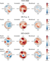 |
Fig. 2 Reconstructed large-scale magnetic field maps of TOI-1860, DS Tuc A, and HD 63433 in flattened polar view. For completeness, we included our previous HD 63433 reconstruction using 2023 data (Bellotti et al. 2024). From the left, the radial, azimuthal, and meridional components of the magnetic field vector are illustrated. Concentric circles represent different stellar latitudes: −30°, +30°, and +60° (dashed lines), as well as the equator (solid line). The radial ticks are located at the rotational phases when the observations were collected. The rotational phases are computed with Eq. (3). The colour bar indicates the polarity and strength (in G) of the magnetic field. |
5 Stellar wind
We simulated the stellar wind of TOI-1860, DS Tuc A, and HD 63433 using the Space Weather Modelling Framework (SWMF, Tóth et al. 2005, 2012) and specifically the Alfvén wave solar model (AWSoM, Sokolov et al. 2013; van der Holst et al. 2014) applied to the ZDI reconstructions described in Sect 4. A detailed description of the methodology behind the wind models can be found in the recent works of Ó Fionnagáin et al. (2019), Kavanagh et al. (2019), Evensberget et al. (2021), Alvarado-Gómez et al. (2022), Evensberget et al. (2022), Boro Saikia et al. (2023) and Evensberget et al. (2023). Here, we briefly summarise the main features of the model. The three-dimensional simulations of the stellar wind are performed by numerically solving the ideal two-temperature magnetohydrodynamic equations, letting the models converge towards a steady state solution in which balance between the magnetic and hydrodynamic forces is reached across the domain of the simulation (a summary of the equations is given in Evensberget et al. 2021).
Our AWSoM model extends from the chromosphere (that is, the inner boundary), where the temperature is set at 5 × 10⁴ K and the number density is set at 2 × 10¹¹ m−3, through the transition region to the stellar corona. In the AWSoM model, the stellar corona is heated by dissipation of Alfvén waves emanating from deeper stellar layers, resulting in a Poynting flux ΠA proportional to the local |B| value at the inner model boundary. Boro Saikia et al. (2023) used FUV emission lines forming in the chromosphere and the transition region to measure the velocity associated to the non-thermal processes that drive the solar and stellar wind. They found that the non-thermal velocities of Sun-like stars can have similar values as that observed in the solar chromosphere and transition region, hence we expect the energy density of Alfvén waves to resemble that of the Sun. The propagation and partial reflection of the Alfvén waves results in a turbulent cascade that heats and accelerates the solar wind (van der Holst et al. 2014; Gombosi et al. 2018). We set the Poynting flux-to-field ratio to 1.1 × 10⁵ erg cm−2 G−1, the same one as used in solar wind models, and the turbulence correlation length to 1.5 × 10⁹ m T1/2.
The models fixes the large-scale radial field component at the inner boundary to the ZDI-derived values (see Fig. 2), while the transverse components are left to evolve as the numerical solution relaxes towards steady state. We emphasise that, except for the stellar mass, radius, rotation period and large-scale magnetic field, the input parameters of the AWSoM model were set to solar values that have been shown to reproduce solar wind conditions (Meng et al. 2015; van der Holst et al. 2019; Sachdeva et al. 2019).
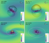 |
Fig. 3 Simulated stellar wind of TOI-1860, DS Tuc A, and HD 63433 in the x⋆ − y⋆ plane. The rotation axis lies along the positive z⋆. The Alfvén surface is shown as a translucent surface and its intersection on the x⋆ − y⋆ plane is shown as a white curve. The colour bar indicates the total wind velocity. The orbits of the hosted exoplanets are also included as coloured ellipses. For HD 63433, we also show the simulations from the 2023 data analysed in Bellotti et al. (2024). |
5.1 Characteristics of the wind
The results of our three-dimensional simulations for TOI-1860, DS Tuc A, and HD 63433 are presented in Fig. 3. We also include the simulation of HD 63433 obtained from 2023 data and presented in Bellotti et al. (2024). Each panel is centred on the star and shows the steady-state solution of the stellar wind, colour-coded by the total wind speed ![Mathematical equation: $\[\mathrm{u}_{\text {tot }}=\sqrt{u_{x}^{2}+u_{y}^{2}+u_{z}^{2}}\]$](/articles/aa/full_html/2026/01/aa57581-25/aa57581-25-eq23.png) . Moving away from the star, the wind exhibits a spiral shape owing to stellar rotation, and the wind speed (u) increases while the local wind density (ρw) and magnetic field (Bw) decrease, as expected. The panels also illustrate the Alfvén surface, which is the boundary where the local wind speed matches the Alfvén wave velocity. The latter represents the velocity of magnetic waves propagating through plasma and it is expressed in cgs units as
. Moving away from the star, the wind exhibits a spiral shape owing to stellar rotation, and the wind speed (u) increases while the local wind density (ρw) and magnetic field (Bw) decrease, as expected. The panels also illustrate the Alfvén surface, which is the boundary where the local wind speed matches the Alfvén wave velocity. The latter represents the velocity of magnetic waves propagating through plasma and it is expressed in cgs units as ![Mathematical equation: $\[\mathrm{v}_{\mathrm{A}}=\mathrm{B}_{\mathrm{w}} / \sqrt{4 \pi \rho_{w}}\]$](/articles/aa/full_html/2026/01/aa57581-25/aa57581-25-eq24.png) . As we subsequently discuss in Sect. 5.2, the Alfvén surface is a key factor to determine the possibility of magnetic star-planet interactions (e.g. Vidotto 2025).
. As we subsequently discuss in Sect. 5.2, the Alfvén surface is a key factor to determine the possibility of magnetic star-planet interactions (e.g. Vidotto 2025).
For most of our stars, the Alfvén surface appears predominantly two-lobed, as expected for stars with dominant dipolar large-scale field configurations (e.g. Evensberget et al. 2023). Consistently with the ZDI reconstructions described in Sect. 4, the Alfvén surface of HD 63433 features a larger and more complex shape than TOI-1860 and DS Tuc A, and then our previous wind simulation of HD 63433 corresponding to 2023 data (see Bellotti et al. 2024). This temporal evolution of the Alfvén surface, which correlates with the evolution of the large-scale magnetic field, can modulate magnetic star-planet interactions.
We computed the mass loss rate (![Mathematical equation: $\[\dot{\text{M}}\]$](/articles/aa/full_html/2026/01/aa57581-25/aa57581-25-eq25.png) ) by integrating the mass flux over a closed spherical surface (Σ) centred on the star
) by integrating the mass flux over a closed spherical surface (Σ) centred on the star
![Mathematical equation: $\[\dot{\mathrm{M}}=\oint_{\Sigma} \rho ~\mathbf{u} \cdot \hat{\mathbf{n}} \mathrm{d} ~\Sigma,\]$](/articles/aa/full_html/2026/01/aa57581-25/aa57581-25-eq26.png) (4)
(4)
where ρ and u are the stellar wind density and speed of our steady-state solution. As listed in Table 3, we estimated values between 5 and 20 times larger than the solar wind-mass loss rate. We note that ![Mathematical equation: $\[\dot{\text{M}}\]$](/articles/aa/full_html/2026/01/aa57581-25/aa57581-25-eq27.png) should not vary with the choice of surface Σ, as long as such surface encloses the star and the model has reached steady state. We found variations for less than 1% by changing the spherical surface radius across the simulation domain, as a numerical check to ensure that the simulation has reached steady-state. The values of
should not vary with the choice of surface Σ, as long as such surface encloses the star and the model has reached steady state. We found variations for less than 1% by changing the spherical surface radius across the simulation domain, as a numerical check to ensure that the simulation has reached steady-state. The values of ![Mathematical equation: $\[\dot{\text{M}}\]$](/articles/aa/full_html/2026/01/aa57581-25/aa57581-25-eq28.png) are reported in Table 3.
are reported in Table 3.
We then computed the angular momentum loss rate (![Mathematical equation: $\[\dot{\text{J}}\]$](/articles/aa/full_html/2026/01/aa57581-25/aa57581-25-eq29.png) ), which regulates the spin-down of the star with age. Following Mestel (1999) and Vidotto et al. (2014),
), which regulates the spin-down of the star with age. Following Mestel (1999) and Vidotto et al. (2014),
![Mathematical equation: $\[\dot{\mathrm{J}}=\oint_{\Sigma}\left[-\frac{\varpi \mathrm{B}_{\varphi} \mathrm{B}_{\mathrm{r}}}{4 \pi}+\varpi \rho \mathrm{u}_{\varphi} \mathrm{u}_{\mathrm{r}}\right] \mathrm{d} \Sigma,\]$](/articles/aa/full_html/2026/01/aa57581-25/aa57581-25-eq30.png) (5)
(5)
where ![Mathematical equation: $\[\varpi=\sqrt{\left(x^{2}+y^{2}\right)}\]$](/articles/aa/full_html/2026/01/aa57581-25/aa57581-25-eq31.png) is the cylindrical radius and (Br, ur) and (Bφ, uφ) are the radial and azimuthal components of the magnetic field and speed of the stellar wind. We estimated values between a factor of 1.4 and 35 larger than the average angular momentum loss rate of the Sun computed for cycle 23–24 (Finley et al. 2019), and all conserved at most within 5%. The values of
is the cylindrical radius and (Br, ur) and (Bφ, uφ) are the radial and azimuthal components of the magnetic field and speed of the stellar wind. We estimated values between a factor of 1.4 and 35 larger than the average angular momentum loss rate of the Sun computed for cycle 23–24 (Finley et al. 2019), and all conserved at most within 5%. The values of ![Mathematical equation: $\[\dot{\text{J}}\]$](/articles/aa/full_html/2026/01/aa57581-25/aa57581-25-eq32.png) are reported in Table 3.
are reported in Table 3.
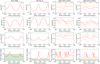 |
Fig. 4 Stellar wind conditions in the planetary frame as a function of stellar rotation phase. From the left, the columns refer to the TOI-1860, DS Tuc A, HD 63433 (2023), and HD 63433 (2024) systems. From the top, the panels show the wind density (ρ), relative velocity (Δu), ram pressure (Pram), and Alfvén Mach number (MA). The sub-Alfvénic regime (MA < 1) of the stellar wind is shown as a green shaded region. In the MA panel of HD 63433, we also show the computation for planet d from 2023 data as a dashed line (see Bellotti et al. 2024). |
5.2 Environment at the planetary orbit
We now describe the stellar wind characteristics at the orbits of the known exoplanets, which are illustrated in Fig. 3 as coloured ellipses around the stars. Quantitative information of the wind conditions at these orbits and the location relative to the Alfvén surface are shown in Fig. 4. Using the planetary frame as a reference, we computed the variations of wind density, relative speed (Δu), ram pressure and Alfvén Mach number during one stellar rotation. The relative speed is between the wind velocity and the Keplerian velocity of the planet Δu = u − vK, and it is used to compute the ram pressure experienced by the planet Pram = ρwΔu2. The Alfvén Mach number is the ratio between the Alfvén wave velocity and the wind speed, MA = Δu/vA, and it is a practical quantity to determine whether an orbit is in sub-Alfvénic regime MA < 1 or in super-Alfvénic regime MA > 1.
TOI-1860 is a young (133 Myr) K1-type star hosting one known planet at 0.02 au or 1.066 d orbit as revealed by TESS observations (Giacalone et al. 2022). The planet radius is 1.31 R⊕, the equilibrium temperature is 1885 K and the authors estimated a mass of 2.2 M⊕ from the probabilistic relation of Chen & Kipping (2017). The eccentricity of the planetary orbit has not been constrained yet in the literature, hence we assumed a circular orbit in the equatorial plane of the star with radius equal to 4.66 R⋆ (with R⋆ = 0.94 R⊙). As shown in the first column of Fig. 4, the average wind density and speed are 7.9 × 10⁻¹⁹ g/cm3 and 260 km/s, and the planet experiences an average ram pressure of 4.2 × 10⁻⁴ dyn/cm2. The two dips (or peaks) stem from the spiral morphology of the wind, which is in turn shaped by the change of polarity of the dipolar component. The orbit of TOI-1860 b is predominantly sub-Alfvénic and becomes super-Alfvénic briefly between phases 0.23–0.29 and 0.81–0.82.
DS Tuc A is a young (45 Myr) G5-type star in a visual binary system together with the K3-type star DS Tuc B at a separation of 5 arcsec (Torres et al. 2006). The primary component hosts a 5.7 R⊕, super-Neptune planet at an orbital distance of 0.18 au or period of 8.1 d (Newton et al. 2019; Benatti et al. 2019). By modelling radial velocity observations, Benatti et al. (2019) estimated an upper limit on the exoplanet’s mass of 1.3 MNep and they considered the planet to be potentially inflated. Recent simulations by King et al. (2025) of future scenarios for the exoplanet showed that, at 5 Gyr, it may become a Neptune-sized planet or a super-Earth stripped of its primordial H/He envelope. Assuming a circular orbit in the equatorial plane of the star at 20.35 R⋆ (Newton et al. 2019) where R⋆ = 0.96 R⊙, we found an average wind density, speed, and ram pressure of 4.2 × 10⁻²⁰ g/cm3, 430 km/s, and 6.5 × 10⁻⁵ dyn/cm2. We note that these values vary of less than 10% if we assume the orbital distance of 19.42 R⋆ obtained by Benatti et al. (2019). We found that the orbit of the planet is trans-Alfvénic, since parts of it are sub-Alfvénic (orbital phases between 0.07–0.31 and 0.58–0.83) while the rest is super-Alfvénic.
HD 63433 is a young (414 Myr) G5-type star hosting three planets at 0.05 au (planet d), 0.07 au (planet b), 0.14 au (planet c Capistrant et al. 2024). The orbital periods are 4.2 d, 7.11 d, and 20.55 d, and the radii are 1.07 R⊕, 2.02 R⊕, and 2.44 R⊕ (see also Mann et al. 2020; Mallorquín et al. 2023; Damasso et al. 2023). From radial velocity observations, Damasso et al. (2023) measured planetary mass upper limits of 11 M⊕ for planet b and 31 M⊕ for planet c, while Mallorquín et al. (2023) measured 22 M⊕ for planet b and 15.5 M⊕ for planet c.
Following Bellotti et al. (2024), we assumed that the planets have circular orbits in the equatorial plane of the star with radii of 16.8 R⋆, 36.1 R⋆, and 9.9 R⋆ for planet b, c, and d (with R⋆ = 0.897 R⊙). For planet b, the average wind density, speed, and ram pressure are 2.9 × 10⁻²⁰ g/cm3, 250 km/s, and 1.7 × 10⁻⁵ dyn/cm2. For planet c, these values are 5.3 × 10⁻²¹ g/cm3, 275 km/s, and 3.9 × 10⁻⁶ dyn/cm2. For planet d, these values are 1.2 × 10⁻¹⁹ g/cm3, 214 km/s, and 5.1 × 10⁻⁵ dyn/cm2.
As for the 2023 observations, the orbits of planet b and c are super-Alfénic (see Bellotti et al. 2024). For planet d, the Alfvén surface encompasses a larger fraction of the planetary orbit compared to the simulation of 2023 wind conditions (see Fig. 4), owing to the temporal evolution and intensification of the largescale magnetic field. More specifically, the orbit of planet d was sub-Alfvénic between phases 0.38–0.50, while in our new simulation it is between phases 0.00–0.20, 0.45–0.69, and 0.86–1.00 (see the lower right panel of Fig. 4).
6 Conclusions
With this work, we follow Bellotti et al. (2024) and provide an update on the results of the spectropolarimetric campaign dedicated to characterise the magnetic field of known exoplanet host stars belonging to the current Ariel candidate sample. Our programme aims to collect information on the magnetic activity of a representative sample to inform the observing strategy of Ariel. We analysed spectropolarimetric observations of 15 stars obtained with Neo-Narval, HARPSpol, and SPIRou.
We did not detect circularly polarised Zeeman signatures in eight stars over multiple snapshot observations. We detected Zeeman signatures for TOI-1136, TOI-1860, DS Tuc A, and the newest observations of HD 63433, and we obtained one marginal detection for TOI-836 and two for TOI-2076. We estimated absolute longitudinal magnetic field values of the order of 5–50 G for these stars, which is in agreement with previous studies of fast-rotating, solar-like stars (e.g. Petit et al. 2005, 2008; Marsden et al. 2014; Folsom et al. 2016; Brown et al. 2022).
We performed the reconstruction of the large-scale magnetic field via ZDI for TOI-1860, DS Tuc A, and HD 63433, but not TOI-1136, since we did not have a sufficient number of observations. For TOI-1860 and DS Tuc A, this is the first reconstruction of the large-scale magnetic field. For TOI-1860, we found a predominantly toroidal and moderately axisymmetric large-scale magnetic field with an average strength of 37 G. For DS Tuc A, we found a poloidal magnetic field that is mostly dipolar and axisymmetric with an average field strength of 64 G. For HD 63433, our new 2024 observations revealed a more complex topology compared to the 2023 map, with more energy stored in the ℓ = 3 and ℓ = 4 modes at the expenses of the ℓ = 1 mode. The other features are similar: ~50% poloidal, moderately axisymmetric and with an average field strength of 70 G. In a broader context, the ZDI reconstructions of these stars are in agreement with the large-scale field configuration of young, solar-like stars which are known to exhibit variability also of the order of one year (see Folsom et al. 2016; Willamo et al. 2022; Bellotti et al. 2025a, for recent examples).
Finally, we used the magnetic field reconstructions to numerically model the stellar wind environment and compute the location of the Alfvén surface. As expected for dipole-dominated, large-scale magnetic field topologies, the shape of the Alfvén surface is predominantly two-lobed. For HD 63433, the complexity of the large-scale field, that is the deviation from being simply dipolar, translates in a more complex configuration of the Alfvén surface as well. Based on the location of the Alfvén surface, we then evaluated the regime in which the hosted exoplanets are orbiting (see Vidotto 2025, for a recent review).
We found that the orbit of TOI-1860 b is almost completely sub-Alfvénic, meaning that a direct connection between the planet and the stellar magnetic field can occur. As a result, the orbital motion of the planet can generate Alfvén waves propagating towards the star or magnetic reconnection events (e.g. Neubauer 1998; Ip et al. 2004; Saur et al. 2013; Strugarek et al. 2015; Kavanagh et al. 2022). From the recent work of Presa et al. (2024), assuming the planetary magnetic field to be dipolar and with a certain obliquity, we expect the planet atmospheric escape in sub-Alfvénic regime to occur via a single polar outflow, which was found to be weaker than the bipolar outflow typical of super-Alfvénic interactions (Carolan et al. 2021a). We also note that, given the young age of the system, XUV irradiation would also be an important source of atmospheric mass loss.
There are several ways with which the stellar wind can affect atmospheric escape in exoplanets. They can reduce escape rates (Vidotto & Cleary 2020), change signatures of atmospheric evaporation through spectroscopic transits (Carolan et al. 2021b), and possibly generate a tenuous atmosphere through sputtering processes (Vidotto et al. 2018). With the constrained stellar wind properties presented in our work, future atmospheric models of exoplanets will be able to better pin-point the effects of the wind of the host star on the planet’s upper atmosphere, as well as potential signatures in Ly-α and He I transits. For Ariel specifically, such models are important to assess the presence and evolution of an exoplanet atmosphere (Kubyshkina et al. 2022), as well as to interpret the planetary atmospheric response to stellar activity (e.g. upper-atmosphere heating, ionisation, and chemistry García Muñoz 2023; Strugarek et al. 2025).
The orbits of HD 63433 b and c are super-Alfvénic, in a similar manner as the previous stellar wind model from 2023 data (see Bellotti et al. 2024). In this regime, which is reminiscent of the regime in which Solar System planets orbit, we expect the formation of a bow shock between a potential planetary magnetosphere and the stellar wind (Chapman & Ferraro 1931; Vidotto et al. 2009, 2010), as well as the presence of evaporated planetary material in the shape of a tail (e.g. Schneiter et al. 2007; Villarreal D’Angelo et al. 2018). Finally, planets DS Tuc A b and HD 63433 d are in the trans-Alfvénic region, where the stellar wind conditions can alternate between super- and sub-Alfvénic. For HD 63433 d, we note that sub-Alfvénic fraction of the orbit is increased relative to the model from 2023 data, owing to the temporal variability of the stellar large-scale magnetic field. Finally, we also note that the Alfvén surface in our model is mostly dictated by the ratio between the Poynting flux and the magnetic field strength reconstructed with ZDI. Such reconstructions may lead to an underestimated magnetic field strength (Lehmann et al. 2019), ultimately affecting the size of the Alfvén surface (see e.g. Fig. 5 Kavanagh et al. 2021).
At this point, additional observations are required to confirm whether the large-scale magnetic field is detectable for certain exoplanet host stars. An example of uncertain magnetic field detection is TOI-2076, for which we found two marginal detections and four non-detections, while Damasso et al. (2024) corroborated its magnetic activity and a long-term variation of ~2.7 yr. Furthermore, our results motivate the spectropolarimetric monitoring of the presented sub-sample of potential Ariel stars on the long-term. Such a monitoring can address the question of whether the stars manifest magnetic cycles and if so, how they relate to the activity cycles discovered with other techniques. For instance, DS Tuc A exhibits a long-term photometric variation of ~8 yr, as described by Benatti et al. (2019). Ultimately, this will be valuable to constrain the temporal evolution of the Alfvén surface and of the observational signatures marking magnetic star-planet interactions, as well as the evolution of evaporating atmospheres and their interactions with the stellar wind.
The spectropolarimetric programme presented here started in 2022 and it is expected to continue until the launch of Ariel, with the aim of informing observing strategies for specific targets as well as atmospheric modelling. Once the mission is launched, the goal of the campaign will become of a follow-up nature, thus complementing the observations already performed and providing new insights for the interpretation of Ariel data. The Ariel Candidate Sample is subject to yearly adjustments based on new analyses of the most suitable targets for atmospheric characterisation, but also in light of new exoplanet discoveries. Although it is hard to estimate a number of targets given the dynamic nature of the Candidate Sample combined with our selection criteria for magnetically active stars, we expect between two and five additional stars per year, for which to assess the magnetic field detectability and reconstruct the topology.
Data availability
The spectropolarimetric observations analysed in this work are available on online databases. All Neo-Narval and SPIRou observations are available on PolarBase8 (Petit et al. 2014). The Neo-Narval observations were taken under the programmes L232N02, L241N09, and L251N08 and the SPIRou observations under the programmes 22BF97, 23AF16, 23BF98, and 24AF99. The HARPSPol observations are available at the ESO Science Archive9 under the programmes 110.24C8.001, 110.24C8.002, 115.28DD.001, and 115.28DD.002.
Acknowledgements
This publication is part of the project “Exo-space weather and contemporaneous signatures of star-planet interactions” (with project number OCENW.M.22.215 of the research programme “Open Competition Domain Science-M”), which is financed by the Dutch Research Council (NWO). This work used the Dutch national e-infrastructure with the support of the SURF Cooperative using grant nos. EINF-2218 and EINF-5173. This work has been developed within the framework of the Ariel “Stellar Characterisation” and “Stellar Activity” working groups, in synergy with the “Planetary Formation” working group of the ESA Ariel space mission Consortium. AAV and DE acknowledge funding from the European Research Council (ERC) under the European Union’s Horizon 2020 research and innovation programme (grant agreement No 817540, ASTROFLOW). AAV acknowledges funding from the Dutch Research Council (NWO), with project number VI.C.232.041 of the Talent Programme Vici. C.D. acknowledges financial support from the grant RYC2023-044903-I funded by MCIU/AEI/10.13039/501100011033 and by the ESF+. We thank the TBL team for providing service observing with Neo-Narval under the programmes L232N02, L241N09, and L251N08 (PI S. Bellotti). Based on observations obtained at the Canada-France-Hawaii Telescope (CFHT) which is operated by the National Research Council of Canada, the Institut National des Sciences de l’Univers of the Centre National de la Recherche Scientique of France, and the University of Hawaii. The observations were collected under the programmes 22BF97, 23AF16, 23BF98, and 24AF99 (PI S. Bellotti and P. Petit). Based on observations collected at the European Southern Observatory under ESO programmes 110.24C8.001, 110.24C8.002, 115.28DD.001, and 115.28DD.002 (PI: S. Bellotti). This research has made use of the NASA Exoplanet Archive, which is operated by the California Institute of Technology, under contract with the National Aeronautics and Space Administration under the Exoplanet Exploration Program. This work made use of the Ariel Stellar Catalogue developed by the Stellar Characterisation WG in preparation of the ESA Ariel space mission. This work used the BATS-R-US tools developed at the University of Michigan Center for Space Environment Modeling and made available through the NASA Community Coordinated Modeling Center. This work has made use of the VALD database, operated at Uppsala University, the Institute of Astronomy RAS in Moscow, and the University of Vienna; Astropy, 12 a community-developed core Python package for Astronomy (Astropy Collaboration 2013, 2018); NumPy (van der Walt et al. 2011); Matplotlib: Visualization with Python (Hunter 2007); SciPy (Virtanen et al. 2020) and PyAstronomy (Czesla et al. 2019).
References
- Alvarado-Gómez, J. D., Hussain, G. A. J., Grunhut, J., et al. 2015, A&A, 582, A38 [NASA ADS] [CrossRef] [EDP Sciences] [Google Scholar]
- Alvarado-Gómez, J. D., Cohen, O., Drake, J. J., et al. 2022, ApJ, 928, 147 [CrossRef] [Google Scholar]
- Angus, R., Morton, T., Aigrain, S., Foreman-Mackey, D., & Rajpaul, V. 2018, MNRAS, 474, 2094 [Google Scholar]
- Astropy Collaboration (Robitaille, T. P., et al.) 2013, A&A, 558, A33 [NASA ADS] [CrossRef] [EDP Sciences] [Google Scholar]
- Astropy Collaboration (Price-Whelan, A. M., et al.) 2018, AJ, 156, 123 [Google Scholar]
- Bagnulo, S., Landolfi, M., Landstreet, J. D., et al. 2009, PASP, 121, 993 [Google Scholar]
- Bellotti, S., Fares, R., Vidotto, A. A., et al. 2023a, A&A, 676, A139 [NASA ADS] [CrossRef] [EDP Sciences] [Google Scholar]
- Bellotti, S., Morin, J., Lehmann, L. T., et al. 2023b, A&A, 676, A56 [NASA ADS] [CrossRef] [EDP Sciences] [Google Scholar]
- Bellotti, S., Evensberget, D., Vidotto, A. A., et al. 2024, A&A, 688, A63 [NASA ADS] [CrossRef] [EDP Sciences] [Google Scholar]
- Bellotti, S., Lüftinger, T., Boro Saikia, S., et al. 2025a, A&A, 700, A282 [NASA ADS] [CrossRef] [EDP Sciences] [Google Scholar]
- Bellotti, S., Petit, P., Jeffers, S. V., et al. 2025b, A&A, 693, A269 [NASA ADS] [CrossRef] [EDP Sciences] [Google Scholar]
- Benatti, S., Nardiello, D., Malavolta, L., et al. 2019, A&A, 630, A81 [NASA ADS] [CrossRef] [EDP Sciences] [Google Scholar]
- Boro Saikia, S., Lueftinger, T., Jeffers, S. V., et al. 2018, A&A, 620, L11 [NASA ADS] [CrossRef] [EDP Sciences] [Google Scholar]
- Boro Saikia, S., Lueftinger, T., Airapetian, V. S., et al. 2023, ApJ, 950, 124 [NASA ADS] [CrossRef] [Google Scholar]
- Brown, E. L., Jeffers, S. V., Marsden, S. C., et al. 2022, MNRAS, 514, 4300 [CrossRef] [Google Scholar]
- Canto Martins, B. L., Gomes, R. L., Messias, Y. S., et al. 2020, ApJS, 250, 20 [NASA ADS] [CrossRef] [Google Scholar]
- Capistrant, B. K., Soares-Furtado, M., Vanderburg, A., et al. 2024, AJ, 167, 54 [NASA ADS] [CrossRef] [Google Scholar]
- Carolan, S., Vidotto, A. A., Hazra, G., Villarreal D’Angelo, C., & Kubyshkina, D. 2021a, MNRAS, 508, 6001 [NASA ADS] [CrossRef] [Google Scholar]
- Carolan, S., Vidotto, A. A., Villarreal D’Angelo, C., & Hazra, G. 2021b, MNRAS, 500, 3382 [Google Scholar]
- Changeat, Q., Keyte, L., Waldmann, I. P., & Tinetti, G. 2020, ApJ, 896, 107 [NASA ADS] [CrossRef] [Google Scholar]
- Chapman, S., & Ferraro, V. C. A. 1931, Terrestr. Magn. Atmos. Electr. (J. Geophys. Res.), 36, 77 [Google Scholar]
- Chen, J., & Kipping, D. 2017, ApJ, 834, 17 [Google Scholar]
- Claret, A., & Bloemen, S. 2011, A&A, 529, A75 [NASA ADS] [CrossRef] [EDP Sciences] [Google Scholar]
- Cook, N. J., Artigau, É., Doyon, R., et al. 2022, PASP, 134, 114509 [NASA ADS] [CrossRef] [Google Scholar]
- Cotton, D. V., Evensberget, D., Marsden, S. C., et al. 2019, MNRAS, 483, 1574 [NASA ADS] [CrossRef] [Google Scholar]
- Czesla, S., Schröter, S., Schneider, C. P., et al. 2019, PyA: Python astronomy-related packages [Google Scholar]
- Dai, F., Masuda, K., Beard, C., et al. 2023, AJ, 165, 33 [NASA ADS] [CrossRef] [Google Scholar]
- Damasso, M., Locci, D., Benatti, S., et al. 2023, A&A, 672, A126 [NASA ADS] [CrossRef] [EDP Sciences] [Google Scholar]
- Damasso, M., Locci, D., Benatti, S., et al. 2024, A&A, 690, A235 [NASA ADS] [CrossRef] [EDP Sciences] [Google Scholar]
- Danielski, C., Brucalassi, A., Benatti, S., et al. 2022, Exp. Astron., 53, 473 [NASA ADS] [CrossRef] [Google Scholar]
- Di Maio, C., Changeat, Q., Benatti, S., & Micela, G. 2023, A&A, 669, A150 [NASA ADS] [CrossRef] [EDP Sciences] [Google Scholar]
- Donati, J. F. 2003, in Astronomical Society of the Pacific Conference Series, 307, Solar Polarization, eds. J. Trujillo-Bueno, & J. Sanchez Almeida, 41 [Google Scholar]
- Donati, J. F., & Brown, S. F. 1997, A&A, 326, 1135 [Google Scholar]
- Donati, J. F., Semel, M., Carter, B. D., Rees, D. E., & Collier Cameron, A. 1997, MNRAS, 291, 658 [Google Scholar]
- Donati, J. F., Mengel, M., Carter, B. D., et al. 2000, MNRAS, 316, 699 [Google Scholar]
- Donati, J.-F., Forveille, T., Collier Cameron, A., et al. 2006, Science, 311, 633 [Google Scholar]
- Donati, J. F., Kouach, D., Moutou, C., et al. 2020, MNRAS, 498, 5684 [Google Scholar]
- Donati, J.-F., Cristofari, P. I., Finociety, B., et al. 2023, MNRAS, 525, 455 [NASA ADS] [CrossRef] [Google Scholar]
- Edwards, B., & Tinetti, G. 2022, AJ, 164, 15 [NASA ADS] [CrossRef] [Google Scholar]
- Edwards, B., Mugnai, L., Tinetti, G., Pascale, E., & Sarkar, S. 2019, AJ, 157, 242 [NASA ADS] [CrossRef] [Google Scholar]
- Evensberget, D., Carter, B. D., Marsden, S. C., Brookshaw, L., & Folsom, C. P. 2021, MNRAS, 506, 2309 [NASA ADS] [CrossRef] [Google Scholar]
- Evensberget, D., Carter, B. D., Marsden, S. C., et al. 2022, MNRAS, 510, 5226 [NASA ADS] [CrossRef] [Google Scholar]
- Evensberget, D., Marsden, S. C., Carter, B. D., et al. 2023, MNRAS, 524, 2042 [CrossRef] [Google Scholar]
- Finley, A. J., Hewitt, A. L., Matt, S. P., et al. 2019, ApJ, 885, L30 [NASA ADS] [CrossRef] [Google Scholar]
- Folsom, C. P., Petit, P., Bouvier, J., et al. 2016, MNRAS, 457, 580 [Google Scholar]
- Folsom, C. P., Bouvier, J., Petit, P., et al. 2018, MNRAS, 474, 4956 [NASA ADS] [CrossRef] [Google Scholar]
- Folsom, C. P. Ó Fionnagáin, D., Fossati, L., et al. 2020, A&A, 633, A48 [NASA ADS] [CrossRef] [EDP Sciences] [Google Scholar]
- Folsom, C. P., Erba, C., Petit, V., et al. 2025, J. Open Source Softw., 10, 7891 [Google Scholar]
- Frazier, R. C., Stefánsson, G., Mahadevan, S., et al. 2023, ApJ, 944, L41 [NASA ADS] [CrossRef] [Google Scholar]
- García Muñoz, A. 2023, A&A, 672, A77 [NASA ADS] [CrossRef] [EDP Sciences] [Google Scholar]
- Garraffo, C., Drake, J. J., & Cohen, O. 2016, ApJ, 833, L4 [NASA ADS] [CrossRef] [Google Scholar]
- Genest, F., Lafrenière, D., Boucher, A., et al. 2022, AJ, 163, 231 [NASA ADS] [CrossRef] [Google Scholar]
- Giacalone, S., Dressing, C. D., Hedges, C., et al. 2022, AJ, 163, 99 [NASA ADS] [CrossRef] [Google Scholar]
- Gombosi, T. I., van der Holst, B., Manchester, W. B., & Sokolov, I. V. 2018, Liv. Rev. Sol. Phys., 15, 4 [CrossRef] [Google Scholar]
- Güdel, M. 2004, A&A Rev., 12, 71 [Google Scholar]
- Hahlin, A., Kochukhov, O., Rains, A. D., et al. 2023, A&A, 675, A91 [NASA ADS] [CrossRef] [EDP Sciences] [Google Scholar]
- Hara, N. C., Bouchy, F., Stalport, M., et al. 2020, A&A, 636, L6 [NASA ADS] [CrossRef] [EDP Sciences] [Google Scholar]
- Hawthorn, F., Bayliss, D., Wilson, T. G., et al. 2023, MNRAS, 520, 3649 [NASA ADS] [CrossRef] [Google Scholar]
- Hazra, G., Vidotto, A. A., & D’Angelo, C. V. 2020, MNRAS, 496, 4017 [NASA ADS] [CrossRef] [Google Scholar]
- Hunter, J. D. 2007, Comput. Sci. Eng., 9, 90 [NASA ADS] [CrossRef] [Google Scholar]
- Hussain, G. A. J., Collier Cameron, A., Jardine, M. M., et al. 2009, MNRAS, 398, 189 [Google Scholar]
- Ip, W.-H., Kopp, A., & Hu, J.-H. 2004, ApJ, 602, L53 [NASA ADS] [CrossRef] [Google Scholar]
- Johnstone, C. P., Bartel, M., & Güdel, M. 2021, A&A, 649, A96 [EDP Sciences] [Google Scholar]
- Kavanagh, R. D., Vidotto, A. A., Ó Fionnagáin, D., et al. 2019, MNRAS, 485, 4529 [NASA ADS] [CrossRef] [Google Scholar]
- Kavanagh, R. D., Vidotto, A. A., Klein, B., et al. 2021, MNRAS, 504, 1511 [Google Scholar]
- Kavanagh, R. D., Vidotto, A. A., Vedantham, H. K., et al. 2022, MNRAS, 514, 675 [CrossRef] [Google Scholar]
- King, G. W., Corrales, L. R., Bourrier, V., et al. 2025, ApJ, 980, 27 [Google Scholar]
- Klein, B., Donati, J.-F., Moutou, C., et al. 2021, MNRAS, 502, 188 [Google Scholar]
- Kochukhov, O., Hackman, T., Lehtinen, J. J., & Wehrhahn, A. 2020, A&A, 635, A142 [NASA ADS] [CrossRef] [EDP Sciences] [Google Scholar]
- Kochukhov, O., Makaganiuk, V., & Piskunov, N. 2010, A&A, 524, A5 [NASA ADS] [CrossRef] [EDP Sciences] [Google Scholar]
- Kubyshkina, D., Vidotto, A. A., Villarreal D’Angelo, C., et al. 2022, MNRAS, 510, 2111 [Google Scholar]
- Lammer, H., Selsis, F., Ribas, I., et al. 2003, ApJ, 598, L121 [Google Scholar]
- Landi Degl’Innocenti, E. 1992, Magnetic Field Measurements, eds. F. Sanchez, M. Collados, & M. Vazquez, 71 [Google Scholar]
- Lanza, A. F. 2013, A&A, 557, A31 [NASA ADS] [CrossRef] [EDP Sciences] [Google Scholar]
- Lehmann, L. T., & Donati, J. F. 2022, MNRAS, 514, 2333 [CrossRef] [Google Scholar]
- Lehmann, L. T., Hussain, G. A. J., Jardine, M. M., Mackay, D. H., & Vidotto, A. A. 2019, MNRAS, 483, 5246 [Google Scholar]
- Lehmann, L. T., Donati, J. F., Fouqué, P., et al. 2024, MNRAS, 527, 4330 [Google Scholar]
- Locci, D., Aresu, G., Petralia, A., et al. 2024, Planet. Sci. J., 5, 58 [Google Scholar]
- Locci, D., Petralia, A., Micela, G., et al. 2022, Planet. Sci. J., 3, 1 [NASA ADS] [CrossRef] [Google Scholar]
- López Ariste, A., Georgiev, S., Mathias, P., et al. 2022, A&A, 661, A91 [NASA ADS] [CrossRef] [EDP Sciences] [Google Scholar]
- Luque, R., Fulton, B. J., Kunimoto, M., et al. 2022, A&A, 664, A199 [NASA ADS] [CrossRef] [EDP Sciences] [Google Scholar]
- Magrini, L., Danielski, C., Bossini, D., et al. 2022, A&A, 663, A161 [NASA ADS] [CrossRef] [EDP Sciences] [Google Scholar]
- Mallorquín, M., Béjar, V. J. S., Lodieu, N., et al. 2023, A&A, 671, A163 [NASA ADS] [CrossRef] [EDP Sciences] [Google Scholar]
- Mancini, L., Esposito, M., Covino, E., et al. 2018, A&A, 613, A41 [NASA ADS] [CrossRef] [EDP Sciences] [Google Scholar]
- Mann, A. W., Johnson, M. C., Vanderburg, A., et al. 2020, AJ, 160, 179 [Google Scholar]
- Marsden, S. C., Petit, P., Jeffers, S. V., et al. 2014, MNRAS, 444, 3517 [Google Scholar]
- Mayor, M., Pepe, F., Queloz, D., et al. 2003, The Messenger, 114, 20 [NASA ADS] [Google Scholar]
- Mazeh, T., Perets, H. B., McQuillan, A., & Goldstein, E. S. 2015, ApJ, 801, 3 [Google Scholar]
- McCann, J., Murray-Clay, R. A., Kratter, K., & Krumholz, M. R. 2019, ApJ, 873, 89 [NASA ADS] [CrossRef] [Google Scholar]
- McComas, D. J. 2003, in American Institute of Physics Conference Series, 679, Solar Wind Ten, eds. M. Velli, R. Bruno, F. Malara, & B. Bucci (AIP), 33 [Google Scholar]
- Meng, X., van der Holst, B., Tóth, G., & Gombosi, T. I. 2015, MNRAS, 454, 3697 [NASA ADS] [CrossRef] [Google Scholar]
- Mestel, L. 1999, Stellar magnetism [Google Scholar]
- Moutou, C., Donati, J. F., Savalle, R., et al. 2007, A&A, 473, 651 [NASA ADS] [CrossRef] [EDP Sciences] [Google Scholar]
- Mugnai, L. V., Pascale, E., Edwards, B., Papageorgiou, A., & Sarkar, S. 2020, Exp. Astron., 50, 303 [NASA ADS] [CrossRef] [Google Scholar]
- Neubauer, F. M. 1998, J. Geophys. Res., 103, 19843 [NASA ADS] [CrossRef] [Google Scholar]
- Newton, E. R., Mann, A. W., Tofflemire, B. M., et al. 2019, ApJ, 880, L17 [Google Scholar]
- Nicholson, B. A., Vidotto, A. A., Mengel, M., et al. 2016, MNRAS, 459, 1907 [CrossRef] [Google Scholar]
- Ó Fionnagáin, D., Vidotto, A. A., Petit, P., et al. 2019, MNRAS, 483, 873 [NASA ADS] [Google Scholar]
- Osborn, H. P., Bonfanti, A., Gandolfi, D., et al. 2022, A&A, 664, A156 [NASA ADS] [CrossRef] [EDP Sciences] [Google Scholar]
- Oshagh, M., Santos, N. C., Boisse, I., et al. 2013, A&A, 556, A19 [NASA ADS] [CrossRef] [EDP Sciences] [Google Scholar]
- Petit, P., Donati, J. F., & Collier Cameron, A. 2002, MNRAS, 334, 374 [NASA ADS] [CrossRef] [Google Scholar]
- Petit, P., Donati, J. F., Aurière, M., et al. 2005, MNRAS, 361, 837 [Google Scholar]
- Petit, P., Dintrans, B., Solanki, S. K., et al. 2008, MNRAS, 388, 80 [NASA ADS] [CrossRef] [Google Scholar]
- Petit, P., Louge, T., Théado, S., et al. 2014, PASP, 126, 469 [NASA ADS] [CrossRef] [Google Scholar]
- Piskunov, N. E., & Valenti, J. A. 2002, A&A, 385, 1095 [NASA ADS] [CrossRef] [EDP Sciences] [Google Scholar]
- Piskunov, N., Snik, F., Dolgopolov, A., et al. 2011, The Messenger, 143, 7 [NASA ADS] [Google Scholar]
- Piskunov, N., Wehrhahn, A., & Marquart, T. 2021, A&A, 646, A32 [NASA ADS] [CrossRef] [EDP Sciences] [Google Scholar]
- Pizzolato, N., Maggio, A., Micela, G., Sciortino, S., & Ventura, P. 2003, A&A, 397, 147 [NASA ADS] [CrossRef] [EDP Sciences] [Google Scholar]
- Pont, F., Gilliland, R. L., Moutou, C., et al. 2007, A&A, 476, 1347 [NASA ADS] [CrossRef] [EDP Sciences] [Google Scholar]
- Pont, F., Sing, D. K., Gibson, N. P., et al. 2013, MNRAS, 432, 2917 [NASA ADS] [CrossRef] [Google Scholar]
- Presa, A., Driessen, F. A., & Vidotto, A. A. 2024, MNRAS, 534, 3622 [Google Scholar]
- Press, W. H., Teukolsky, S. A., Vetterling, W. T., & Flannery, B. P. 1992, Numerical recipes in FORTRAN. The art of scientific computing [Google Scholar]
- Rackham, B. V., Apai, D., & Giampapa, M. S. 2018, ApJ, 853, 122 [Google Scholar]
- Rackham, B. V., Apai, D., & Giampapa, M. S. 2019, AJ, 157, 96 [Google Scholar]
- Rees, D. E., & Semel, M. D. 1979, A&A, 74, 1 [NASA ADS] [Google Scholar]
- Reiners, A., Shulyak, D., Käpylä, P. J., et al. 2022, A&A, 662, A41 [NASA ADS] [CrossRef] [EDP Sciences] [Google Scholar]
- Reinhold, T., & Hekker, S. 2020, A&A, 635, A43 [NASA ADS] [CrossRef] [EDP Sciences] [Google Scholar]
- Rusomarov, N., Kochukhov, O., Piskunov, N., et al. 2013, A&A, 558, A8 [NASA ADS] [CrossRef] [EDP Sciences] [Google Scholar]
- Ryabchikova, T., Piskunov, N., Kurucz, R. L., et al. 2015, Phys. Scr., 90, 054005 [Google Scholar]
- Sachdeva, N., van der Holst, B., Manchester, W. B., et al. 2019, ApJ, 887, 83 [NASA ADS] [CrossRef] [Google Scholar]
- Salz, M., Czesla, S., Schneider, P. C., et al. 2018, A&A, 620, A97 [NASA ADS] [CrossRef] [EDP Sciences] [Google Scholar]
- Saur, J., Grambusch, T., Duling, S., Neubauer, F. M., & Simon, S. 2013, A&A, 552, A119 [NASA ADS] [CrossRef] [EDP Sciences] [Google Scholar]
- Schneiter, E. M., Velázquez, P. F., Esquivel, A., Raga, A. C., & Blanco-Cano, X. 2007, ApJ, 671, L57 [NASA ADS] [CrossRef] [Google Scholar]
- Schrijver, C. J., & Zwaan, C. 2000, Solar and Stellar Magnetic Activity [Google Scholar]
- Semel, M. 1989, A&A, 225, 456 [NASA ADS] [Google Scholar]
- Skilling, J., & Bryan, R. K. 1984, MNRAS, 211, 111 [NASA ADS] [CrossRef] [Google Scholar]
- Snik, F., Kochukhov, O., Piskunov, N., et al. 2011, in Astronomical Society of the Pacific Conference Series, 437, Solar Polarization 6, eds. J. R. Kuhn, D. M. Harrington, H. Lin, S. V. Berdyugina, J. Trujillo-Bueno, S. L. Keil, & T. Rimmele, 237 [Google Scholar]
- Sokolov, I. V., van der Holst, B., Oran, R., et al. 2013, ApJ, 764, 23 [NASA ADS] [CrossRef] [Google Scholar]
- Spina, L., Nordlander, T., Casey, A. R., et al. 2020, ApJ, 895, 52 [Google Scholar]
- Strugarek, A., Brun, A. S., Matt, S. P., & Réville, V. 2015, ApJ, 815, 111 [Google Scholar]
- Strugarek, A., García Muñoz, A., Brun, A. S., & Paul, A. 2025, A&A, 693, A220 [NASA ADS] [CrossRef] [EDP Sciences] [Google Scholar]
- Tessore, B., Lèbre, A., Morin, J., et al. 2017, A&A, 603, A129 [NASA ADS] [CrossRef] [EDP Sciences] [Google Scholar]
- Tinetti, G., Drossart, P., Eccleston, P., et al. 2018, Exp. Astron., 46, 135 [NASA ADS] [CrossRef] [Google Scholar]
- Tinetti, G., Eccleston, P., Lueftinger, T., et al. 2022, in European Planetary Science Congress, EPSC2022-1114 [Google Scholar]
- Torres, C. A. O., Quast, G. R., da Silva, L., et al. 2006, A&A, 460, 695 [NASA ADS] [CrossRef] [EDP Sciences] [Google Scholar]
- Tóth, G., Sokolov, I. V., Gombosi, T. I., et al. 2005, J. Geophys. Res. (Space Phys.), 110, A12226 [Google Scholar]
- Tóth, G., van der Holst, B., Sokolov, I. V., et al. 2012, J. Computat. Phys., 231, 870 [Google Scholar]
- Tsantaki, M., Magrini, L., Danielski, C., et al. 2025, A&A, 697, A102 [NASA ADS] [CrossRef] [EDP Sciences] [Google Scholar]
- van der Holst, B., Sokolov, I. V., Meng, X., et al. 2014, ApJ, 782, 81 [Google Scholar]
- van der Holst, B., Manchester, W. B. I., Klein, K. G., & Kasper, J. C. 2019, ApJ, 872, L18 [NASA ADS] [CrossRef] [Google Scholar]
- van der Walt, S., Colbert, S. C., & Varoquaux, G. 2011, Comput. Sci. Eng., 13, 22 [Google Scholar]
- Van Looveren, G., Boro Saikia, S., Herbort, O., et al. 2025, A&A, 694, A310 [NASA ADS] [CrossRef] [EDP Sciences] [Google Scholar]
- Vidotto, A. A. 2025, ARA&A, 63, 299 [Google Scholar]
- Vidotto, A. A., & Cleary, A. 2020, MNRAS, 494, 2417 [Google Scholar]
- Vidotto, A. A., Opher, M., Jatenco-Pereira, V., & Gombosi, T. I. 2009, ApJ, 703, 1734 [NASA ADS] [CrossRef] [Google Scholar]
- Vidotto, A. A., Jardine, M., & Helling, C. 2010, ApJ, 722, L168 [NASA ADS] [CrossRef] [Google Scholar]
- Vidotto, A. A., Fares, R., Jardine, M., et al. 2012, MNRAS, 423, 3285 [NASA ADS] [CrossRef] [Google Scholar]
- Vidotto, A. A., Jardine, M., Morin, J., et al. 2014, MNRAS, 438, 1162 [Google Scholar]
- Vidotto, A. A., Fares, R., Jardine, M., Moutou, C., & Donati, J. F. 2015, MNRAS, 449, 4117 [NASA ADS] [CrossRef] [Google Scholar]
- Vidotto, A. A., Lichtenegger, H., Fossati, L., et al. 2018, MNRAS, 481, 5296 [Google Scholar]
- Vidotto, A. A., Bourrier, V., Fares, R., et al. 2023, A&A, 678, A152 [NASA ADS] [CrossRef] [EDP Sciences] [Google Scholar]
- Villarreal D’Angelo, C., Esquivel, A., Schneiter, M., & Sgró, M. A. 2018, MNRAS, 479, 3115 [CrossRef] [Google Scholar]
- Virtanen, P., Gommers, R., Burovski, E., et al. 2020, scipy/scipy: SciPy 1.5.3 [Google Scholar]
- Willamo, T., Lehtinen, J. J., Hackman, T., et al. 2022, A&A, 659, A71 [NASA ADS] [CrossRef] [EDP Sciences] [Google Scholar]
- Zingales, T., Tinetti, G., Pillitteri, I., et al. 2018, Exp. Astron., 46, 67 [NASA ADS] [CrossRef] [Google Scholar]
The mission candidate sample is available here: https://github.com/arielmission-space/Mission_Candidate_Sample
Available at https://github.com/folsomcp/LSDpy
Appendix A Additional figures
In this appendix we provide the observed Stokes V LSD profiles used for the ZDI reconstruction and their Unno-Rachkovsky models. Fig. A.1 shows the Stokes V LSD profiles for TOI-1860, DS Tuc A, and HD 63433 analysed in this work.
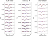 |
Fig. A.1 Time series of Stokes V LSD profiles and the ZDI models for TOI-1860, DS Tuc A, and HD 63433. The observations are shown in black and the models in red. The numbers on the right indicate the rotational cycle computed from Eq. 3 using the first observation of an epoch as reference date for DS Tuc A and the median observation for TOI-1860 and HD 63433. The horizontal line represents the zero point of the profiles, which are shifted vertically based on their rotational phase for visualisation purposes. |
Appendix B Journal of observations
In this appendix, we provide a list of the observations performed with Neo-Narval, HARPSpol, and SPIRou. We also list the value of the longitudinal magnetic field (Bℓ).
Journal of observations
All Tables
All Figures
|
Fig. 1 Joint search of differential rotation and equatorial rotation period for TOI-1860 (top) and HD 63433 (bottom). The panels illustrate the |
| In the text | |
|
Fig. 2 Reconstructed large-scale magnetic field maps of TOI-1860, DS Tuc A, and HD 63433 in flattened polar view. For completeness, we included our previous HD 63433 reconstruction using 2023 data (Bellotti et al. 2024). From the left, the radial, azimuthal, and meridional components of the magnetic field vector are illustrated. Concentric circles represent different stellar latitudes: −30°, +30°, and +60° (dashed lines), as well as the equator (solid line). The radial ticks are located at the rotational phases when the observations were collected. The rotational phases are computed with Eq. (3). The colour bar indicates the polarity and strength (in G) of the magnetic field. |
| In the text | |
|
Fig. 3 Simulated stellar wind of TOI-1860, DS Tuc A, and HD 63433 in the x⋆ − y⋆ plane. The rotation axis lies along the positive z⋆. The Alfvén surface is shown as a translucent surface and its intersection on the x⋆ − y⋆ plane is shown as a white curve. The colour bar indicates the total wind velocity. The orbits of the hosted exoplanets are also included as coloured ellipses. For HD 63433, we also show the simulations from the 2023 data analysed in Bellotti et al. (2024). |
| In the text | |
|
Fig. 4 Stellar wind conditions in the planetary frame as a function of stellar rotation phase. From the left, the columns refer to the TOI-1860, DS Tuc A, HD 63433 (2023), and HD 63433 (2024) systems. From the top, the panels show the wind density (ρ), relative velocity (Δu), ram pressure (Pram), and Alfvén Mach number (MA). The sub-Alfvénic regime (MA < 1) of the stellar wind is shown as a green shaded region. In the MA panel of HD 63433, we also show the computation for planet d from 2023 data as a dashed line (see Bellotti et al. 2024). |
| In the text | |
|
Fig. A.1 Time series of Stokes V LSD profiles and the ZDI models for TOI-1860, DS Tuc A, and HD 63433. The observations are shown in black and the models in red. The numbers on the right indicate the rotational cycle computed from Eq. 3 using the first observation of an epoch as reference date for DS Tuc A and the median observation for TOI-1860 and HD 63433. The horizontal line represents the zero point of the profiles, which are shifted vertically based on their rotational phase for visualisation purposes. |
| In the text | |
Current usage metrics show cumulative count of Article Views (full-text article views including HTML views, PDF and ePub downloads, according to the available data) and Abstracts Views on Vision4Press platform.
Data correspond to usage on the plateform after 2015. The current usage metrics is available 48-96 hours after online publication and is updated daily on week days.
Initial download of the metrics may take a while.