| Issue |
A&A
Volume 705, January 2026
|
|
|---|---|---|
| Article Number | A257 | |
| Number of page(s) | 7 | |
| Section | Extragalactic astronomy | |
| DOI | https://doi.org/10.1051/0004-6361/202557643 | |
| Published online | 23 January 2026 | |
The X-ray/UV connection in NGC 5548: A rapidly varying corona
1
Department of Physics, University of Crete 71003 Heraklion, Greece
2
Institute of Astrophysics, FORTH GR-71110 Heraklion, Greece
3
Department of Physics and Institute of Theoretical and Computational Physics, University of Crete 71003 Heraklion, Greece
4
MIT Kavli Institute for Astrophysics and Space Research, Massachusetts Institute of Technology Cambridge MA 02139, USA
5
Cahill Center for Astronomy and Astrophysics, California Institute of Technology 1200 California Boulevard Pasadena CA 91125, USA
6
Astronomical Institute of the Academy of Sciences Boční II 1401 CZ-14100 Prague, Czech Republic
★ Corresponding author: This email address is being protected from spambots. You need JavaScript enabled to view it.
Received:
10
October
2025
Accepted:
4
December
2025
Abstract
Recent intensive monitoring campaigns of active galactic nuclei have provided simultaneous X-ray, UV, and optical data of unprecedented quality. The observations revealed a strong correlation between the UV and optical variability, but a weaker correlation between the X-ray and UV bands. This challenges the standard X-ray reprocessing scenario. We revisit the X-ray/UV connection in NGC 5548 by fitting archival 2014 HST and Swift/XRT light curves assuming X-ray reverberation from a dynamically evolving X-ray corona. Our results show that as long as the corona height, photon index, and power vary over time, X-ray reverberation can explain the observed UV and optical variability within 2% and 5%, respectively (on average). The evolution of the best-fit parameters suggests that fast changes in coronal geometry and energetics on a timescale of days are required to explain the observed variability.
Key words: accretion / accretion disks / galaxies: active / galaxies: Seyfert / X-rays: galaxies / X-rays: individuals: NGC 5548
© The Authors 2026
 Open Access article, published by EDP Sciences, under the terms of the Creative Commons Attribution License (https://creativecommons.org/licenses/by/4.0), which permits unrestricted use, distribution, and reproduction in any medium, provided the original work is properly cited.
This article is published in open access under the Subscribe to Open model. This email address is being protected from spambots. You need JavaScript enabled to view it. to support open access publication.
1. Introduction
Active galactic nuclei (AGN) exhibit variable X-ray and UV/optical emission across a range of timescales. The X-rays vary faster at short timescales. The physical mechanism that causes the X-ray/UV/optical variability in AGN has been the focus of intensive study. Clavel et al. (1992) were among the first to study the X-ray/UV variability in AGN by performing simultaneous X-ray and UV observations of NGC 5548. They observed correlated X-ray and UV variations, which they attributed to X-ray reverberation of the accretion disc. More recently, NGC 5548 was monitored by Swift over a two-year period (from 03/2012 to 02/2014 McHardy et al. 2014). These observations showed a good correlation overall between the X-ray and UV/optical bands with the UV/optical bands lagging the X-ray band with delays that increase with wavelength. This is consistent with expectations from X-ray reverberation. The measured lag amplitudes, however, were found to be larger than expected.
Similar results were also reached by Edelson et al. (2015), Fausnaugh et al. (2016), and Edelson et al. (2019), who studied the X-ray/UV and optical variability of NGC 5548 using the light curves from the AGN Space Telescope and Optical Reverberation Mapping (STORM) campaign (De Rosa et al. 2015). This was a dense and long monitoring campaign, involving Swift, HST, and many ground-based telescopes. Many more monitoring campaigns of Seyferts have been conducted since then (see Cackett et al. 2021 and Paolillo & Papadakis 2025 for a recent review of these campaigns). The NGC 5548 observations revealed strong and well-correlated UV/optical variability, but the time lags where again longer than predicted by standard disc reprocessing. Neustadt & Kochanek (2022) suggested that temperature fluctuations that slowly propagate through the accretion flow on timescales far longer than the light-travel time might explain these observations.
Since then, alternative ideas have been proposed to account for the longer than expected UV/optical time lags. For example, Netzer (2022) suggested that the observed time lags in NGC 5548 (and other Seyferts) are due to the response of the diffuse gas in the broad line region to the variable ionising continuum. Cai et al. (2020) attributed the observed time lags to disc turbulences when the effect of large-scale turbulence is considered. Furthermore, Hagen et al. (2024) suggested that the observed time lags in Fairall 9 are due to the reverberation of the variable EUV from an inner wind, which produces a lagged bound-free continuum that matches the observed UV/optical lags.
Despite the initial suggestions, X-ray reverberation in the lamp-post geometry can explain the UV/optical time delays (Kammoun et al. 2021b, 2023), the power spectrum in the UV/optical bands (Panagiotou et al. 2022b), and the frequency-resolved time lags (Panagiotou et al. 2025) of NGC 5548 using the STORM light curves. The same model can also fit the mean UV/optical/X-ray spectral energy distribution (SED) of the source (Dovčiak et al. 2022). These results suggest that at least in NGC 5548, X-ray reverberation can explain the observed UV/optical variations.
An issue remains that might suggest otherwise, however. The X-ray to UV correlation is weaker than the UV to optical correlation (Edelson et al. 2015, 2019). The X-ray light curve does not visually appear to be the driver of the UV/optical light curves. Starkey et al. (2017) showed that the inferred driving light curve reconstructed from UV/optical data did not match the observed X-ray light curve, while Gardner & Done (2017) found that X-ray reverberation of a standard accretion disc resulted in simulated UV/optical light curves that reproduced too much of the hard X-ray high-frequency power. More recently, Mahmoud & Done (2020), Mahmoud et al. (2023) and Hagen & Done (2023) showed similar discrepancies between the X-ray reverberating disc signal and the observed UV light curves in NGC 4151, Ark 120, and Fairall 9, respectively. They proposed that intrinsic fluctuations within the accretion disc and not direct X-ray reprocessing dominate the observed UV variability.
Panagiotou et al. (2022a) showed that a dynamic corona can explain the possibility of a low cross-correlation between the X-ray and UV/optical light curves in the case of X-ray reverberation. Kammoun et al. (2024) (K24 hereafter) further demonstrated that the time-variable SEDs of NGC5548 can be well reproduced by X-ray reverberation in the case of a dynamic corona, even in the presence of a weak X-ray/UV flux correlation.
We adopt a complementary approach by fitting the full light curves of NGC5548. This allows us to explore the temporal evolution of the disc–corona system in more detail. In particular, we show that the observed UV (and optical) light curves of NGC 5548 during the STORM campaign can be naturally explained by reprocessing of X-rays emitted from a dynamical X-ray corona in the lamp-post geometry, where the corona power, height, and photon index are variable. Section 2 introduces our reverberation model, followed by a description of the observational data in Section 3. The fitting procedure is detailed in Section 4, and the results are presented in Section 5. Finally, we discuss our findings in Section 6.
2. The X-ray reverberation model
We considered an X-ray source that illuminates an accretion disc. Part of the X-rays falling on the disc are re-emitted in X-rays, and the other part is absorbed by the disc and acts as an additional source of heating. In this way, the disc emission is connected with the X-ray emission. In a steady-state system, this connection can be expressed as
 (1)
(1)
where Fλ(t) is the total flux of the disc at wavelength λ and time t, Fλ, NT is the constant flux of a standard accretion disc without illumination (Novikov & Thorne 1973), LX(t) is the luminosity of the X-rays at time t, and Ψλ(t) is the disc response function, which describes how the disc responds to the illumination of X-rays (see Kammoun et al. 2021a, 2023). The shape and amplitude of the response function depend on all the physical parameters of the accretion disc/X-ray system, such as the black hole (BH) mass, the accretion rate, the height, and the luminosity of the X-ray source. These parameters may not be constant over time, and as a result, the response function evolves over time. In this dynamic system, the disc emission can be estimated by generalising the above equation (Panagiotou et al. 2022a)
 (2)
(2)
where t0 = 0, and N is the number of times that Ψ(t) changes. In this equation, we assume that Ψ(t) remains constant within the time interval (ti, ti + 1), while N can be arbitrarily large.
3. The light curves
We are interested in the UV and X-ray light curves of NGC 5548. We first present the HST UV continuum light curves and then the X-ray light curve derived from Swift/XRT observations.
3.1. The UV light curves
For the UV, we used the HST H1 (λ = 1158 Å), H3 (λ = 1479 Å), and H4 (λ = 1746 Å) continuum light curves of Fausnaugh et al. (2016) (i.e. the shortest, middle, and longest wavelength HST light curves of the STORM campaign). We only considered the far UV light curves because the convolution integral in Eq. (2) can be computed fast in this case because the width of the disc response is small (∼1 day) at these short wavelengths. In addition, they are not contaminated by the host galaxy light and by construction are not expected to include any contribution by emission lines.
We corrected the light curves for Galactic extinction with E(B − V) = 0.0171 (Schlafly & Finkbeiner 2011) and the extinction law of Cardelli et al. (1989). We also corrected for absorption from the host galaxy, assuming E(B − V)host = 0.14, as determined by K24, and the extinction law of Czerny et al. (2004). The open grey squares in panels (b), (c), and (d) of Fig. 2 show the resulting H1, H3, and H4 band light curves, respectively.
3.2. The X-ray light curve
The X-ray luminosity in Eq. (2) refers to the X-ray luminosity in the 2–10 keV band. To compute it, we calculated the flux in the 2–10 keV band by fitting the X-ray spectrum of each observation. We used the automatic Swift/XRT data products generator1 (Evans et al. 2009) to extract the X-ray spectrum of each observation. We grouped each spectrum to have at least 15 counts per bin and fit the spectra in XSPEC (Arnaud 1996) with an absorbed power-law model of the form
 (3)
(3)
The TBabs component (Wilms et al. 2000) quantifies the X-ray absorption by our own Galaxy, and we fixed the column density to NH = 1.55 × 1020 cm−2 (HI4PI Collaboration 2016). The second neutral absorber, zTBabs, accounts for absorption from the host galaxy, and we fixed its column density to NH, host = 8.3 × 10²¹ E(B − V)host = 12 × 1020 cm−2 (Liszt 2021). We also included a warm absorber using zxipcf (Reeves et al. 2008). Since NGC 5548 exhibits variable ionised obscuration in X-rays (e.g. Mehdipour et al. 2016; Dehghanian et al. 2019), we allowed the column density, Nwa, and the ionisation parameter of the warm absorber, log(ξ), to vary freely during the fit. The quality of the individual spectra prevented us from letting the covering fraction vary as well, and we therefore fixed it to unity.
Figure 1 shows the Swift/XRT spectrum of two observations: one observation with a count rate of 0.2 (black points, ID 00030022237; exposure 964 s), and another with count rate of 0.6 (red points, ID 00033204104; exposure 570 s). They are representative of the low and high count rate spectra of the campaign. The best-fit models (defined by Eq. (3)) are shown with the black and red lines, while the best-fit residuals are shown in the bottom panel. The best-fit parameters for the low and high count rate spectra are  cm−2, log
 ,
,  , and
, and  cm−2, log
 , and
, and  . The errors were estimated using the error command in XSPEC for Δχ2 = 2.71, which corresponds to the 90% confidence range for a single parameter of interest. They can be large, but the main purpose of fitting the individual spectra is to compute the 2–10 keV unabsorbed X-ray flux (and then luminosity) of the source.
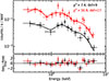 |
Fig. 1. Swift/XRT spectra for an observation with a low count rate (black points) and an observation with a high count rate (red points). The black and red lines show the best-fitting model of Eq. (3). The bottom panel shows the best-fit residuals. |
We used the cflux component to compute the 2–10 keV flux,  , and its error,
  (estimated as explained above for the best-fit parameters). The unabsorbed flux calculated from the best-fit model to the spectra plotted in Fig. 1 is 6.3 ± 1.8 × 10⁻¹¹ and
  erg/s/cm2 for the low and high count rate spectra, respectively. The grey squares in the top panel of Fig. 2 show the resulting
  as a function of time for the whole monitoring campaign. We note that in some cases, the flux error was quite large due to the poor quality of the single-observation spectra. For this reason, we omitted the points with
  (∼10% of the total points; these points are not shown in Fig. 2).
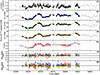 |
Fig. 2. Observed 2–10 keV, H1, H3, H4, and B-band light curves (open grey squares in panels (a), (b), (c), (d), and (e)). The black open squares and the filled coloured circles show the observations we considered in the fitting procedure and the best-fit model predictions, respectively. Panels (f) and (g) show the data-model/data and data-model/error ratios for the X-ray, H1, H3, H4, and B-band light curves (black, blue, green, orange, and red circles, respectively). |
In addition to the statistical error of the flux measurements, systematic uncertainties may also be present when the X-ray absorption is not modelled properly. To test this, we assumed that the warm absorber is not variable and recalculated the unabsorbed flux of each observation using the best-fit values reported in Table 2 of K24, which were estimated when fitting the mean spectrum of the source (Nwa = 2.54 × 1022 cm−2, log(ξ) = 1.37). The  values did not vary by more than ∼25%. This difference was almost always smaller than the error of the flux measurements.
The X-ray flux measurements include contributions from the primary emission and the X-ray reflected component from the accretion disc. We only needed the primary emission for our modelling, however. We attempted to unravel the primary and reflected components by modelling the reflection with xillver (García et al. 2016) and refitting the spectra. The statistical quality of individual spectra is low, however, and prevents us from constraining the reflected flux. We therefore assumed that 10% of the observed X-ray flux arises from reflection and 90% from the primary emission. This assumption is supported by the spectral modelling of the mean SED of NGC 5548 using KYNSED (Dovčiak et al. 2022) in K24, which indicates that the reflected component contributes about 10% of the observed 2–10 keV flux. We further verified that our best-fit results were consistent with this assumption a posteriori using KYNSED, as explained in Sect. 5.
4. The X-ray reverberation modelling of the UV light curves
We used the relativistic reverberation model KYNXiltr (Kammoun et al. 2023) to compute Ψλ(t). In summary, a lamp-post geometry was assumed for the X-ray source, whose emission follows a power law with a slope of Γint and a high-energy exponential roll-off, which we fixed at Ecut = 150 keV (Ursini et al. 2015). We fixed the mass of the central BH at MBH = 7 × 10⁷ M⊙ (Horne et al. 2021), the inclination of the disc at θ = 40° (Pancoast et al. 2014), and the distance at DL = 80.1 Mpc according to the NASA/IPAC Extragalactic Database (NED). For the BH spin, the colour correction factor, and the accretion rate (in Eddington units), we accepted α* = 0, fcol = 1.7 (the best-fit values in K24), and ṁEdd = 0.06. We also tested the cases of ṁEdd = 0.05 and 0.07 and found that a value of 0.06 fits the UV light curves better. The free parameters were the height of the X-ray source, h, the photon index Γint, and the ratio Ltransf/Ldisc, where Ldisc is the power released by the accretion process in the disc and Ltransf is the luminosity of the X-ray corona, which we assumed to be equal to the accretion power released in the disc below a certain radius rtransf (Kammoun et al. 2023).
We note that the photon index of the corona emission, Γint, was left as a free parameter. This is because the best-fit photon index from the spectral modelling of the individual energy spectra, Γobs, cannot be used in our modelling for various reasons. First of all, the X-ray and UV observations are not strictly simultaneous. Secondly, the uncertainty of the Γobs values can be quite large, as discussed in the previous section. In addition, Γobs was estimated from a model that did not include reflection from the disc (and, to a lesser extent, from a distant torus as well). As a result, Γobs might be different from the intrinsic slope of the X-ray spectrum, Γint. Therefore, we needed to let Γint free during the modelling of the UV light curves. Although we were unable to directly use Γobs to constrain Γint, we used  to constrain it (assuming that even when we fit the observed spectra with phenomenological models, the unabsorbed flux we compute is indicative of the intrinsic flux). This can be done using the KYNXiltr code to compute the model flux in the 2–10 keV band,
  , which depends on Γint, and then fit the unabsorbed
  light curve simultaneously with the UV light curves.
We computed the disc response function using a uniformly sampled grid of model parameters, with 20 linearly spaced values for each of the free parameters: the coronal height h, ranging from 5 to 50 rg, Ltransf/Ldisc from 0.3 to 0.9, and the photon index Γint from 1.3 to 2.1. These parameter ranges are motivated by the best-fit values of K24. To compute Fλ(t) using Eq. (2), we also needed the disc flux when the disc is not illuminated by the X-rays, Fλ, NT(t). We calculated this using KYNSED, with the same model parameters as above. Fλ, NT(t) can also be variable when Ltransf/Ldisc is variable. The last parameter that we needed was LX. As we mentioned previously, LX in this equation refers to the 2–10 keV band X-ray luminosity. This is equal to  , where the factor of 0.9 accounts for the fact that we only needed the primary emission, as discussed in the previous section.
To reliably predict the observed UV flux measurements using the convolution integral of Eq. (2) requires well-sampled X-ray observations (roughly two per day) over a period of ∼3 days preceding each UV data point. The black boxes in panels (b), (c), and (d) of Fig. 2 highlight the HST measurements that meet this requirement. These are the points included in our fits (91 in each light curve). We started from MJD 56713 because the first ∼25 days of the X-ray light curve are too sparsely sampled. This is also the case with the last ∼40 days of the X-ray light curve, whereas the gaps in the X-ray light curve around MJD 56773, 56780, and 56815 also prevent the model prediction of the UV flux at these times.
For each set of model parameter values, we computed the model fluxes in the H1, H3, and H4 bands using Eq. (2). The width of the response functions in these bands is small, and we therefore stopped the calculation of the convolution integral in Eq. (2) at t′ = 3 days. This choice significantly increased the computational efficiency of the model fitting process and did not compromise the accuracy of the model estimates (we verified that contributions from longer times are below ∼1%).
For the first HST measurements at t = 56713 MJD, the convolution reduces to the simpler expression in Eq. (1). The best-fit model parameters at this time were determined by minimising the weighted squared error (WSE) between the model and the observed H1, H3, H4 and  fluxes,
 (4)
(4)
We adopted the WSE approach as it enables a comparison between model and data in terms of fractional differences, without relying on potentially unreliable or underestimated observational uncertainties. This method also ensures that the X-ray light curve contributes to the overall fit as much as a UV light curve, even though the error bars are larger.
As we explained above, we fit  together with the UV light curves, mainly to constrain Γint. We note that because the Swift and HST observations are not simultaneous, we used linear interpolation to compute
  at each time of the UV light curve points. The black boxes in the top panel of Fig. 2 show the interpolated
  values. When the best-fit parameters (i.e. h, Ltransf/Ldisc, and Γint) were obtained for the first time point, we proceeded iteratively using Eq. (2) to fit the next light curve point by finding the parameters that produced the minimum WSE. In this way, the value of the model parameters only varied at the times when the HST observations were made, but not between.
5. Best-fit results
Figure 2 shows our best-fitting results. The black points in the top panel of Fig. 2 show the best fit 2–10 keV flux, while the blue, green, and orange points in panels (b), (c), and (d) show the best-fit H1, H3, and H4 light curves, respectively. Panel (f) shows the ratio (data-model)/data. We also plot the best-fit residuals (i.e. (data-model)/error) in panel (g).
Figure 2 shows that X-ray reverberation is able to explain all the observed variability features in the UV light curves rather well at all sampled timescales. The plot of the best-fit ratio residuals (panel (f) in Fig. 2) demonstrates that the model reproduces the X-ray and UV data with an accuracy better than 10% throughout the monitoring period and captures all variability features of the light curves. The average absolute residuals are ∼3% for the H1 light curve and ∼2% for the 2–10 keV, H3 and H4 light curves. This shows that the model and observations agree well. The best-fit χ2 is 517 for 91 degrees of freedom2, however. From a statistical standpoint, this result indicates that the model does not fit the data well. The χ2 results indicate that the unaccounted 2–3% of the observed variations (on average) are highly significant (assuming the photometric errors are determined correctly). When we add a systematic error of 4% in quadrature, the best-fit χ2 reduces to 110, which implies a good fit to the data with a null hypothesis probability of 0.09. We computed the excess variance of the H1, H3, and H4 light curves using only the points we modelled, and their average variability amplitude (i.e. the square root of the excess variance) was 30%, 25%, and 22%, respectively. We therefore conclude that X-ray reverberation can explain most of the observed variations in the UV light curves well. The open squares and filled red circles in panel (e) of Fig. 2 show the SwiftB-band flux measurements during the STORM campaign (Edelson et al. 2015) and the best-fit model predictions. We did not take the B-band data in our model fitting into account because the disc response function in the B-band is much wider than at the UV wavelengths, and the convolution integral in Eq. (2) must therefore be computed up to (at least) t′∼10 days. This considerably increases the computational time required to model the B-band light curve. In addition, there are fewer time intervals of well-sampled X-ray observations (i.e. at least two X-ray observations per day over a period of 10 days) to predict the B-band flux. For this reason, we only plot the best-fit model B-band fluxes over the periods of MJD ∼56729–56770 and ∼56793–56811 in Fig. 2.
Nevertheless, the agreement between the model and the observed B-band light curve is also quite good (the average absolute residual is 5% in this case), although there are some discrepancies. For example, the model systematically underestimates the flux observed between ∼56800–56809 MJD. This might be due to many factors. First, we did not take the (variable) contribution of the emission lines into account, which can be ∼10% in this band (see e.g. Table 8 in Fausnaugh et al. 2016). Secondly, the model assumes a flat disc, which is an oversimplification because the disc height is expected to increase with radius. Even small disc heights can affect the reverberation flux in the optical bands, depending on the value of the model parameters.
5.1. Best-fit parameters
Figure 3 shows the evolution of the best-fit parameters with time3. The top panel shows the height of the X-ray source, the middle panel shows the energy transfer parameter Ltransf/Ldisc, and the bottom panel shows the best-fit photon index Γint. All parameters need to be highly variable to reproduce the observed X-ray and UV variability. The red triangles show the best-fit results of K24, who fitted time-resolved optical/UV/X-ray spectral energy distributions of NGC 5548 using data from the STORM campaign as well.
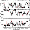 |
Fig. 3. Best-fit parameters. Height (top panel), Ltransf/Ldisc (middle panel), and photon index (bottom panel). The grey shaded area shows the 1σ confidence interval, which we computed by repeating the fitting procedure 100 times, each time resampling the X-ray light curve from Gaussian distributions centred on the measured values with standard deviations equal to their error bar. For computational efficiency, these fits were performed using a coarser parameter grid (i.e. 10 values per parameter instead of 20). The red triangle points show the results of K24. |
Our Γint measurements are very similar to the K24 measurements. These authors fitted the SEDs using KYNSED, which includes the X-ray reflection component in the X-ray band. This result indicates that the Γint values we derived from the light curve fitting are consistent with those obtained from the spectral modelling. In general, the best-fit parameters from both approaches agree very well. For example, 10 (of the 15) of the best-fit h, Ltransf/Ldisc, and Γint values are consistent within 1σ. Only 4 of the (total) 45 best-fit values are outside the 2σ range, and only one of the K24 best-fit values in the bottom panel of Fig. 3 deviates by more than 3σ from our results (the red point at MJD ∼56760 in Fig. 3). The agreement between the best-fit results shows that the two approaches (i.e. fitting time-resolved broad-band SEDs and modelling the observed light curves) are consistent in tracing the evolution of the model parameters and their trends.
5.2. Correlations between the best-fit parameters
The variability of the model parameters shown in Fig. 3 appears to be rather complicated, but some obvious trends are apparent. For example, the large-amplitude flare in the UV and optical band light curves between ∼56735–56755 MJD is mainly due to a systematic variation in Ltransf/Ldisc in the same period. As Ltransf/Ldisc decreases, the disc emission in the UV and optical bands increases (because rtransf decreases), reaching a peak when Ltransf/Ldisc is minimum. Then the UV and optical disc flux decreases as Ltransf/Ldisc increases again. The luminosity of the corona does not drive the UV/optical emission alone, however. For example, the increase in the UV/optical flux observed from ∼56755 to ∼56765 MJD is mainly due to a variation in the height of the corona. During this period, Ltransf/Ldisc remained roughly constant, but the height of the corona increased. As a result, the X-ray flux that illuminates the disc also increased.
Figure 4 shows the correlation between the various best-fit parameters and the observed X-ray and UV fluxes. We modelled these trends with a line in linear or logarithmic space using the ordinary least-squares (OLS) regression method (Isobe et al. 1990). The best-fit lines are shown with solid red lines in the various panels. In most cases, the regression describes the data well. This is further illustrated by the binned averages (black squares; 20 points per bin), which closely follow the best-fit lines.
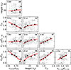 |
Fig. 4. Correlations between the best-fit parameters i.e. the height, the photon index, and the energy transferred to the corona) and the X-ray (2–10 keV) and UV observed fluxes. The red lines show the best-fit straight line or power-law model, and the black squares show the binned data. The numbers in each plot show the significance at which each slope is different from zero. |
Figure 4 is similar to Fig. 8 in K24. Our work is closely related to their work, and both approaches recover similar parameter correlations. Kammoun et al. (2024) constructed broad-band SEDs using data from the STORM campaign and fitted them with KYNSED. They showed that X-ray reverberation can fit the time variable SEDs well, but were able to study only 15 spectra. Our work was performed in the time domain. We were only able to fit three UV light curves, but we used many more observations. Consequently, the panels in Fig. 4 contain many more data points than those in Fig. 8 of K24, which increases the statistical significance of the detected correlations and provides tighter constraints on their evolution.
Many of the apparent correlations in Fig. 4 are statistically significant4. Panel (a) in Fig. 4 shows that the corona height and total X-ray luminosity (i.e. the power transferred to the corona Ltransf/Ldisc) are not correlated. On the other hand, panel (b) of the same figure shows that the spectral slope, Γint, is significantly anti-correlated with the total X-ray luminosity. An increase in X-ray luminosity probably increases the corona temperature (hence the flattening of Γint), but does not affect the corona height. At the same time, the UV flux (i.e.  , where
  is the mean flux) is strongly anti-correlated with the luminosity of the corona (panel g) because we assumed that the corona is powered by the accretion process: When the fraction of the accretion power transferred to the corona decreases, the accretion power available for the heating of the disc increases.
The 2–10 keV X-ray flux appears to be a poor indicator of the total X-ray luminosity, however, as shown by the lack of a strong correlation between the observed F2 − 10 (normalised to its mean,  ) and Ltransf/Ldisc (panel (d) in Fig. 4). We suspect that this is due to two reasons: An increase in total X-ray luminosity should result in an increase in F2 − 10. At the same time, the resulting flattening of Γint should also decrease F2 − 10 (see panel f, which shows the steeper-when-brighter effect in Seyfert galaxies). The two effects probably cancel each other out, causing the lack of correlation between F2 − 10 and the total X-ray luminosity. On the other hand, F2 − 10 appears to correlate broadly with the height of the corona (panel (e) in Fig. 4). The correlation is moderate and appears to hold mainly at low heights (i.e. at heights lower than 15–20 rg). In these cases, as the height increases, more X-ray photons escape to infinity, which causes the increase in the number of the X-ray photons we observe.
Because the UV flux and the X-ray luminosity are anti-correlated (panel (g) of Fig. 4), we would also expect the 2–10 keV and the UV flux to be anti-correlated (in contrast to what is commonly expected) if the 2–10 keV flux were a good indicator of the total X-ray luminosity. Panel (j) suggests a modest positive correlation between F2 − 10 and UV flux, with strong scatter. This explains the small amplitude of the cross-correlation function between the X-ray and UV light curves (e.g. Edelson et al. 2015; Fausnaugh et al. 2016; Edelson et al. 2019). This rather weak and positive correlation probably arises because both F2 − 10 and the UV flux are positively correlated with Γint (mainly) and with the corona height.
We already discussed the correlation between F2 − 10, h, and Γint. Panels (h) and (i) show that the UV flux also correlates with corona height and Γint. The first correlation arises because as the corona height increases, the corona subtends a larger angle to the disc, hence the amount of X-rays illuminating the disc (that are absorbed) increases. The positive correlation between the UV flux and Γint is due to two reasons: Γint is correlated with the total X-ray luminosity, but for a fixed X-ray flux, steeper Γint (slightly) increases the fraction of the flux that is due to X-ray absorption in the UV and optical bands (see Fig. 27 in Kammoun et al. 2021a).
6. Discussion and conclusions
We presented results from the modelling of the HST UV light curves and the Swift/XRT X-ray light curve of NGC5548 during the 2014 STORM campaign, assuming X-ray reverberation from a dynamical X-ray source. The X-ray reverberation within the context of the lamp-post model reproduces the observed light curves to within 2–3% (on average), but only when the X-ray corona properties, that is, the corona height h, the energy transferred from the disc to the corona, Ltransf/Ldisc, and the photon index, Γint, are variable even on timescales of days. Although a direct modelling of the optical light curves is more challenging, the X-ray reverberation model can also describe the B-band light curve well, with residuals of ∼5% on average.
One possible physical explanation for the variations in the corona parameters might be the failed-jet model of Ghisellini et al. (2004). According to this model, radio-quiet AGN emit blobs of material that cannot reach escape velocity. Therefore, they reach a maximum radial distance and then fall back and collide with blobs that were ejected later and still move upward. These collisions dissipate the bulk kinetic energy of the blobs by heating the plasma, hence creating, in effect, X-ray-emitting regions, which naturally have a variable power, height, and photon index. This agrees with our results.
In this model, the X-ray regions can have an intrinsic velocity, and multiple X-ray regions might appear simultaneously at different heights. Given these complexities, the success of our modelling of the observed UV (and optical) variations in NGC 5548 is rather remarkable. The inclusion of more than a single X-ray corona and/or the addition of the intrinsic velocity of the corona with respect to the accretion disc might account for the UV variability amplitude we cannot account for at the moment.
Together with our previous results from the cross-correlation and power spectrum analysis of the STORM light curves, these results suggest that the X-ray reverberation model can account for most of the variability properties of NGC 5548. There are indications that even if X-ray reverberation operates in some Seyferts, it might not be able to explain the full range of observed variations in AGN. For example, Beard et al. (2025) found that X-ray reverberation cannot account for the long-term UV variations in NGC 4395. On the other hand, Papoutsis et al. (2025) showed that X-ray reverberation might cause the very low frequency variations of the SDSS quasars.
A broader examination of mean SEDs, power spectra, and inter-band time lags across a larger sample of sources is needed as a further test of the X-ray reverberation framework. Similarly, modelling the UV and optical light curves of additional Seyfert galaxies might help us to assess whether X-ray reverberation from a dynamical corona can produce the observed UV/optical variability, despite the relatively weak X-ray/UV and optical correlations. These detailed studies of as many sources as possible can show whether X-ray reverberation can explain (at least most of) the observed variations.
Acknowledgments
We thank the referee for their useful comments that helped us improve the manuscript. This work makes use of Matplotlib (Hunter 2007), NumPy (Harris et al. 2020), and SciPy (Virtanen et al. 2020).
References
- Arnaud, K. A. 1996, Astronomical Data Analysis Software and Systems V, 101, 17 [Google Scholar]
- Beard, M. W. J., McHardy, I. M., Horne, K., et al. 2025, MNRAS, 537, 293 [Google Scholar]
- Cackett, E. M., Bentz, M. C., & Kara, E. 2021, iScience, 24, 102557 [NASA ADS] [CrossRef] [Google Scholar]
- Cai, Z.-Y., Wang, J.-X., & Sun, M. 2020, ApJ, 892, 63 [Google Scholar]
- Cardelli, J. A., Clayton, G. C., & Mathis, J. S. 1989, ApJ, 345, 245 [Google Scholar]
- Clavel, J., Nandra, K., Makino, F., et al. 1992, ApJ, 393, 113 [NASA ADS] [CrossRef] [Google Scholar]
- Czerny, B., Li, J., Loska, Z., & Szczerba, R. 2004, MNRAS, 348, L54 [NASA ADS] [CrossRef] [Google Scholar]
- De Rosa, G., Peterson, B. M., Ely, J., et al. 2015, ApJ, 806, 128 [NASA ADS] [CrossRef] [Google Scholar]
- Dehghanian, M., Ferland, G. J., Kriss, G. A., et al. 2019, ApJ, 877, 119 [NASA ADS] [CrossRef] [Google Scholar]
- Dovčiak, M., Papadakis, I. E., Kammoun, E. S., & Zhang, W. 2022, A&A, 661, A135 [NASA ADS] [CrossRef] [EDP Sciences] [Google Scholar]
- Edelson, R., Gelbord, J. M., Horne, K., et al. 2015, ApJ, 806, 129 [NASA ADS] [CrossRef] [Google Scholar]
- Edelson, R., Gelbord, J., Cackett, E., et al. 2019, ApJ, 870, 123 [NASA ADS] [CrossRef] [Google Scholar]
- Evans, P. A., Beardmore, A. P., Page, K. L., et al. 2009, MNRAS, 397, 1177 [Google Scholar]
- Fausnaugh, M. M., Denney, K. D., Barth, A. J., et al. 2016, ApJ, 821, 56 [Google Scholar]
- García, J. A., Fabian, A. C., Kallman, T. R., et al. 2016, MNRAS, 462, 751 [Google Scholar]
- Gardner, E., & Done, C. 2017, MNRAS, 470, 3591 [NASA ADS] [CrossRef] [Google Scholar]
- Ghisellini, G., Haardt, F., & Matt, G. 2004, A&A, 413, 535 [NASA ADS] [CrossRef] [EDP Sciences] [Google Scholar]
- Hagen, S., & Done, C. 2023, MNRAS, 521, 251 [NASA ADS] [CrossRef] [Google Scholar]
- Hagen, S., Done, C., & Edelson, R. 2024, MNRAS, 530, 4850 [Google Scholar]
- Harris, C. R., Millman, K. J., van der Walt, S. J., et al. 2020, Nature, 585, 357 [NASA ADS] [CrossRef] [Google Scholar]
- HI4PI Collaboration. 2016, A&A, 594, A116 [NASA ADS] [CrossRef] [EDP Sciences] [Google Scholar]
- Horne, K., De Rosa, G., Peterson, B. M., et al. 2021, ApJ, 907, 76 [Google Scholar]
- Hunter, J. D. 2007, Comput. Sci. Eng., 9, 90 [NASA ADS] [CrossRef] [Google Scholar]
- Isobe, T., Feigelson, E. D., Akritas, M. G., & Babu, G. J. 1990, ApJ, 364, 104 [Google Scholar]
- Kammoun, E. S., Dovčiak, M., Papadakis, I. E., Caballero-García, M. D., & Karas, V. 2021a, ApJ, 907, 20 [NASA ADS] [CrossRef] [Google Scholar]
- Kammoun, E. S., Papadakis, I. E., & Dovčiak, M. 2021b, MNRAS, 503, 4163 [CrossRef] [Google Scholar]
- Kammoun, E. S., Robin, L., Papadakis, I. E., Dovčiak, M., & Panagiotou, C. 2023, MNRAS, 526, 138 [NASA ADS] [CrossRef] [Google Scholar]
- Kammoun, E., Papadakis, I. E., Dovčiak, M., & Panagiotou, C. 2024, A&A, 686, A69 [NASA ADS] [CrossRef] [EDP Sciences] [Google Scholar]
- Liszt, H. 2021, ApJ, 908, 127 [NASA ADS] [CrossRef] [Google Scholar]
- Mahmoud, R. D., & Done, C. 2020, MNRAS, 491, 5126 [NASA ADS] [Google Scholar]
- Mahmoud, R. D., Done, C., Porquet, D., & Lobban, A. 2023, MNRAS, 521, 3585 [NASA ADS] [CrossRef] [Google Scholar]
- McHardy, I. M., Cameron, D. T., Dwelly, T., et al. 2014, MNRAS, 444, 1469 [NASA ADS] [CrossRef] [Google Scholar]
- Mehdipour, M., Kaastra, J. S., Kriss, G. A., et al. 2016, A&A, 588, A139 [NASA ADS] [CrossRef] [EDP Sciences] [Google Scholar]
- Netzer, H. 2022, MNRAS, 509, 2637 [NASA ADS] [Google Scholar]
- Neustadt, J. M. M., & Kochanek, C. S. 2022, MNRAS, 513, 1046 [NASA ADS] [CrossRef] [Google Scholar]
- Novikov, I. D., & Thorne, K. S. 1973, Black Holes (Les Astres Occlus), 343 [Google Scholar]
- Panagiotou, C., Kara, E., & Dovčiak, M. 2022a, ApJ, 941, 57 [NASA ADS] [CrossRef] [Google Scholar]
- Panagiotou, C., Papadakis, I., Kara, E., Kammoun, E., & Dovčiak, M. 2022b, ApJ, 935, 93 [NASA ADS] [CrossRef] [Google Scholar]
- Panagiotou, C., Papadakis, I., Kara, E., et al. 2025, ApJ, 983, 132 [Google Scholar]
- Pancoast, A., Brewer, B. J., Treu, T., et al. 2014, MNRAS, 445, 3073 [Google Scholar]
- Paolillo, M., & Papadakis, I. 2025, Nuovo Cimento Rivista Serie, 48, 537 [Google Scholar]
- Papoutsis, M., Papadakis, I. E., Panagiotou, C., Kammoun, E., & Dovčiak, M. 2025, A&A, 701, A295 [NASA ADS] [CrossRef] [EDP Sciences] [Google Scholar]
- Reeves, J., Done, C., Pounds, K., et al. 2008, MNRAS, 385, L108 [Google Scholar]
- Schlafly, E. F., & Finkbeiner, D. P. 2011, ApJ, 737, 103 [Google Scholar]
- Starkey, D., Horne, K., Fausnaugh, M. M., et al. 2017, ApJ, 835, 65 [NASA ADS] [CrossRef] [Google Scholar]
- Ursini, F., Boissay, R., Petrucci, P. O., et al. 2015, A&A, 577, A38 [NASA ADS] [CrossRef] [EDP Sciences] [Google Scholar]
- Virtanen, P., Gommers, R., Oliphant, T. E., et al. 2020, Nat. Methods, 17, 261 [Google Scholar]
- Wilms, J., Allen, A., & McCray, R. 2000, ApJ, 542, 914 [Google Scholar]
As we explain in Sect. 4, the model parameters are allowed to vary at each point in the observed light curve, giving in effect 3N free parameters, where N is the number of points in the light curve. Since we considered 4 light curves in the fit, the number of degrees of freedom is 4N − 3N = N.
We checked with KYNSED that the X-ray reflection flux in the 2–10 keV band that the model predicts is ∼10% of the total flux that a distant observer will measure in all cases (i.e. for all the best-fit parameter combinations plotted in Fig. 3). This implies that the best model fit is consistent with our original assumption regarding the fraction of the X-ray reflection flux in the observed spectra.
We consider a correlation significant when the best-fit slope is different from zero by at least 3σ. We compute the error, σ, of the slope by resampling the parameters 1000 times from Gaussian distributions and performing the fit again. We take the standard deviation of the resulting best-fit slope distribution as the slope error.
All Figures
|
Fig. 1. Swift/XRT spectra for an observation with a low count rate (black points) and an observation with a high count rate (red points). The black and red lines show the best-fitting model of Eq. (3). The bottom panel shows the best-fit residuals. |
| In the text | |
|
Fig. 2. Observed 2–10 keV, H1, H3, H4, and B-band light curves (open grey squares in panels (a), (b), (c), (d), and (e)). The black open squares and the filled coloured circles show the observations we considered in the fitting procedure and the best-fit model predictions, respectively. Panels (f) and (g) show the data-model/data and data-model/error ratios for the X-ray, H1, H3, H4, and B-band light curves (black, blue, green, orange, and red circles, respectively). |
| In the text | |
|
Fig. 3. Best-fit parameters. Height (top panel), Ltransf/Ldisc (middle panel), and photon index (bottom panel). The grey shaded area shows the 1σ confidence interval, which we computed by repeating the fitting procedure 100 times, each time resampling the X-ray light curve from Gaussian distributions centred on the measured values with standard deviations equal to their error bar. For computational efficiency, these fits were performed using a coarser parameter grid (i.e. 10 values per parameter instead of 20). The red triangle points show the results of K24. |
| In the text | |
|
Fig. 4. Correlations between the best-fit parameters i.e. the height, the photon index, and the energy transferred to the corona) and the X-ray (2–10 keV) and UV observed fluxes. The red lines show the best-fit straight line or power-law model, and the black squares show the binned data. The numbers in each plot show the significance at which each slope is different from zero. |
| In the text | |
Current usage metrics show cumulative count of Article Views (full-text article views including HTML views, PDF and ePub downloads, according to the available data) and Abstracts Views on Vision4Press platform.
Data correspond to usage on the plateform after 2015. The current usage metrics is available 48-96 hours after online publication and is updated daily on week days.
Initial download of the metrics may take a while.