| Issue |
A&A
Volume 705, January 2026
|
|
|---|---|---|
| Article Number | A243 | |
| Number of page(s) | 16 | |
| Section | Planets, planetary systems, and small bodies | |
| DOI | https://doi.org/10.1051/0004-6361/202557666 | |
| Published online | 23 January 2026 | |
SPIRou detects two planets around the nearby M4.5V star GJ 4274
1
Université de Toulouse, CNRS, IRAP,
14 av. Edouard Belin,
31400
Toulouse,
France
2
Univ. Grenoble Alpes, CNRS, IPAG,
38000
Grenoble,
France
3
SUPA School of Physics and Astronomy, University of St Andrews,
North Haugh,
St Andrews
KY16 9SS,
UK
4
Institut Trottier de recherche sur les exoplanètes, Département de Physique, Université de Montréal,
Montréal,
Québec,
Canada
5
Observatoire du Mont-Mégantic,
Québec,
Canada
6
Institut d’astrophysique de Paris, UMR7095 CNRS, Université Pierre & Marie Curie,
98bis boulevard Arago,
75014
Paris,
France
7
Observatoire de Haute-Provence, CNRS, Université d’Aix-Marseille,
04870
Saint-Michel-l’Observatoire,
France
8
Aix Marseille Univ, CNRS, CNES, LAM,
Marseille,
France
★ Corresponding author: This email address is being protected from spambots. You need JavaScript enabled to view it.
Received:
13
October
2025
Accepted:
31
October
2025
Abstract
Context. M dwarfs are prime targets in the search for exoplanets due to their prevalence and the enhanced radial velocity (RV) detectability of low-mass planets. Recent advancements in instrumentation have extended RV observations from the optical to the near-infrared (nIR) domain, enabling more effective study of M dwarfs, which frequently host rocky planets. The nIR range offers increased RV sensitivity and potentially reduced stellar activity signals, making it particularly well suited for these stars.
Aims. We analyzed spectropolarimetric data of the M4.5V star GJ 4274, acquired using the nIR spectropolarimeter SPIRou, to characterize its stellar activity and to search for planetary signals. We additionally examined TESS photometric data to search for transits corresponding to the potential signals in the RV data.
Methods. In this study, we employed a line-by-line framework to derive and analyze the RV signal of GJ 4274 acquired with SPIRou. From the SPIRou spectra, we also derived and analyzed the longitudinal large scale magnetic field, Bℓ, and the surface temperature variations, dTemp. We combined the SPIRou RV data with RV measurements from CARMENES, to model possible planetary signals with both circular and eccentric orbits. We modeled the activity with a quasiperiodic Gaussian process. We also performed injection-recovery tests on the photometric TESS data to assess transit detectability.
Results. We report the discovery of two exoplanets around the nearby M dwarf star GJ 4274. Both planets are in a circular orbit with respective periods of Pb = 1.6339 ± 0.0001 and Pc = 69.6−1.1+0.3d, the latter located beyond the habitable zone. From their RV semi-amplitude signals (Kb = 5.10−0.67+0.70 m/s and Kc = 4.11 ± 0.64 m/s), we derive minimum masses of mb sin i = 2.97−0.50+0.54M⊕ and mc sin i = 8.4 ± 1.3 M⊕, respectively. Photometric observations from TESS rule out most transit scenarios, including for the inner planet, yielding a maximum inclination of ib ≤ 83° for planet b. We do not detect RV variations related to stellar magnetic activity in the SPIRou time series, despite a prominent large-scale magnetic field with an amplitude of up to ±206−62+158 G. From the activity indicators, we derive a rotation period for the star of 4.600−0.006+0.011d.
Conclusions. The two reported planets belong to the sub-Neptune class. GJ 4274 b has one of the shortest orbital periods among planets orbiting <0.2 M⊙ M dwarfs within 15 pc, while GJ 4274 c lies in a sparsely populated region of the mass–period diagram. Their discovery adds to the census of nearby planetary systems and provides promising targets for future surveys.
Key words: techniques: radial velocities / techniques: spectroscopic
© The Authors 2026
 Open Access article, published by EDP Sciences, under the terms of the Creative Commons Attribution License (https://creativecommons.org/licenses/by/4.0), which permits unrestricted use, distribution, and reproduction in any medium, provided the original work is properly cited.
This article is published in open access under the Subscribe to Open model. This email address is being protected from spambots. You need JavaScript enabled to view it. to support open access publication.
1 Introduction
Nearly 30 years ago, the first exoplanet orbiting a Sun-like star was discovered using the radial velocity (RV) method (Mayor & Queloz 1995). Since then, detection techniques and instrumentation have undergone major advancements. Modern spec-trographs now reach precision levels better than 1 m/s (Fischer et al. 2016; Pepe et al. 2021), opening the door to the detection of low-mass planets. However, the detection of an Earth twin remains a major challenge: the Doppler signal induced by the Earth on the Sun is about 9 cm/s, while stellar activity can introduce several meters per second of RV variability across a broad range of timescales (Meunier et al. 2010; Lagrange et al. 2011; Haywood et al. 2014; Meunier & Lagrange 2019).
M dwarfs are cool, low-mass stars that dominate the local stellar population, accounting for more than 75% of stars within 10 pc (Henry et al. 2006; Reylé et al. 2021). Their small masses and radii enhance the amplitude of planetary RV and transit signals, making them prime targets for detecting and character-izing Earth-mass planets. Statistics from large surveys indicate that M dwarfs typically host multiple low-mass planets (≤ 10 M⊕) (Bonfils et al. 2013; Sabotta et al. 2021; Pinamonti et al. 2022; Mignon et al. 2025), a trend supported by population synthesis models (Burn et al. 2021). Despite this, only approximately 24% of nearby M dwarfs are currently known to host planets within 10 pc from the Sun (Reylé et al. 2021), highlighting the observational challenges posed by their faintness, activity, and the rapid rotation of many late-type members of this population.
To address these challenges and increase detection efficiency, numerous spectroscopic surveys have been launched, including HARPS (High Accuracy Radial velocity Planet Searcher, Bonfils et al. 2013), CARMENES (Calar Alto high-Resolution search for M dwarfs with Exoearths with Near-infrared and optical Échelle Spectrographs, Quirrenbach et al. 2018), HPF (Habitable-Zone Planet Finder, Mahadevan et al. 2012), IRD (InfraRed Doppler, Kotani et al. 2014), MAROON-X (M-dwarf Advanced Radial velocity Observer Of Neighboring eXoplanets, Seifahrt et al. 2018), SOPHIE (Spectrographe pour l’Observation des PHénomènes des Intérieurs stellaires et des Exoplanètes, Bouchy et al. 2013), SPIRou (SpectroPolarimètre InfraRouge, Donati et al. 2020), and NIRPS (Near Infra Red Planet Searcher, Artigau et al. 2024a; Bouchy et al. 2025). These efforts confirm that low-mass planets are common around M dwarfs and suggest that occurrence rates may vary with spectral type (Pinamonti et al. 2022). However, magnetic activity remains a major limitation, particularly in RV measurements (Meunier et al. 2010). Starspots and plages modulated by stellar rotation introduce quasiperiodic signals that can mimic or obscure planetary signatures (Bortle et al. 2021). Notable planetary systems such as Proxima Centauri, GJ 1002, and Gl 699 have nevertheless demonstrated the feasibility of detecting temperate Earth-mass planets around these stars (Anglada-Escudé et al. 2016; Faria et al. 2022; González Hernández et al. 2024; Basant et al. 2025).
Near-infrared (nIR) spectroscopy has become essential for observing M dwarfs, as their flux peaks in this domain and the lower flux contrast between the stellar surface and spots reduces the amplitude of spot-induced RV signals (Martín et al. 2006; Desort et al. 2007; Reiners et al. 2010; Mahmud et al. 2011; Andersen & Korhonen 2015; Cale et al. 2021; Larue et al. 2025). Combined optical and nIR observations further help disentangle chromatic stellar activity from planetary signals (Reiners et al. 2013; Robertson et al. 2020), as shown in cases such as TW Hydrae (Huélamo et al. 2008) and AD Leo (Carleo et al. 2020; Carmona et al. 2023). However, nIR RVs face specific challenges such as telluric absorption (Artigau et al. 2022; Ould-Elhkim et al. 2023), strong magnetic fields (Morin et al. 2010; Kochukhov 2021; Lehmann et al. 2024), and frequent flares (Reiners 2009), which complicate the interpretation of RV variability and require tailored observational strategies and advanced analysis methods.
The SPIRou Legacy Survey Planet Search (SLS-PS; Moutou et al. 2023) spanned 153 observing nights at the Canada-France-Hawaii Telescope (CFHT; 2019a–2022a) aimed at detecting planetary systems around approximately 50 nearby M dwarfs. It was extended through the SPICE program (SPIRou Legacy Survey – Consolidation & Enhancement, 2022b–2024a + PI program in 2024b), with 70.8 additional nights allocated to observe new red dwarfs, while continuing the follow-up on key SLS targets. In this article, we investigate the RV time series of a nearby fully convective star, GJ 4274, observed in the nIR domain with SPIRou1 (Donati et al. 2020). In Section 2, we describe the target, the observational facilities, and the data reduction methods used to derive the RV time series. We discuss stellar activity in Section 3, based on temperature (Artigau et al. 2024b) and longitudinal magnetic field measurements from SPIRou spectropolarimetry. The RVs are then analyzed in Section 4. We then discuss the results in Section 5, before concluding in Section 6.
Stellar parameters of GJ 4274 from the literature.
2 Observations
2.1 GJ 4274
GJ 4274 is an M4.5V star in the solar neighborhood (d = 7.2344 ± 0.0025 pc; Gaia Collaboration 2020). With a low mass of 0.18 ± 0.03 M⊙ (Shan et al. 2024), GJ 4274 is entirely convective (Chabrier & Baraffe 1997). Previous studies by Newton et al. (2018) and Shan et al. (2024) report relatively short rotation periods of 4.591 ± 0.459 d and 4.57 ± 0.04 d, respectively. Because the star is such a fast rotator, its age is expected to be relatively low. From gyro-kinematic studies, Shan et al. (2024) derived an age of 120 Myr. A summary of its stellar parameters reported in the literature is listed in Table 1.
2.2 Observations
Most observations were obtained using SPIRou, a high-resolution near-infrared spectropolarimeter installed in 2018 at the Cassegrain focus of the CFHT. The instrument operates in a spectral range of 0.95−2.50 µm, with a resolving power of 70 000. A detailed overview of the instrumental design and initial performance can be found in Donati et al. (2020). Observations of GJ 4274 with SPIRou span from July 2020 to December 2024, comprising a total of 134 epochs with a median signal-to-noise ratio (S/N) of 101 per night. The mean uncertainty of SPIRou nightly RV measurements is 1.86 m/s. Additionally, we include ten RV measurements acquired using CARMENES (Quirrenbach et al. 2018; Ribas et al. 2023), mostly from July to October 2016, reduced with the SERVAL pipeline (SpEctrum Radial Velocity AnaLyser, Zechmeister et al. 2018). Two were considered outliers, as they deviated significantly and had larger uncertainties. The mean error bar of the remaining points is 1.91 m/s, similar to SPIRou.
This article also includes photometric data obtained with the TESS spacecraft (Ricker et al. 2015). GJ 4274 (referred to as TIC 12652442 in the TESS input catalog, Stassun et al. 2019) was observed during sectors 28 and 42 in August 2020 and August-September 2021. The photometric data obtained were preprocessed by the TESS Science Processing Operations Center (SPOC). The cleaning processes, including removing outliers, de-trending, and correction for systematics, were performed using Lightkurve (Lightkurve Collaboration 2018). The resulting scatter of the processed data corresponds to a precision of 1.58 mmag.
2.3 From SPIRou spectra to precise RV measurements
We reduced all SPIRou spectra using APERO2 (A PipelinE to Reduce Observations), detailed in Cook et al. (2022). The APERO pipeline produces science frames and generates spectra for three fibers: two science channels and one reference channel for calibration3. Within the APERO process, the barycentric Earth radial velocity (BERV) is calculated to shift the wavelengths to the barycentric frame of the Solar System using barycorrpy (Kanodia & Wright 2018). Next, employing the TAPAS model spectrum of the Earth’s atmosphere (Bertaux et al. 2014) and a library of hot star spectra obtained under various air-mass and humidity conditions with SPIRou, APERO performs a three-step telluric correction approach on the science spectra (Cook et al. 2022). For this study, we used the reduced data produced with version 0.7.291 of APERO.
From SPIRou spectra reduced with APERO, we extracted RVs using the line-by-line4 (LBL, v0.65.002) method (Artigau et al. 2022) This method builds on the framework introduced by Bouchy et al. (2001) and Dumusque (2018), further developed for HARPS (Cretignier et al. 2020) and adapted to nIR spectrographs such as SPIRou (Artigau et al. 2022). The LBL method compares each line in the observed spectrum to a template and its derivative to derive RVs, yielding both a mean RV and a per-line RV time series. This per-line information enables advanced statistical analyses, such as weighted principal component analysis (wPCA, Delchambre 2015) used in the wapiti method (Ould-Elhkim et al. 2023). The reduced SPIRou RV measurements are shown in the first panel of Figure 1. Additionally, by extending Bouchy’s equation to higher-order derivatives or projecting it onto physical quantities such as temperature, the framework also provides activity indicators that include the differential line width (dLW; Zechmeister et al. 2018; Artigau et al. 2022; Schöfer et al. 2022) and the differential effective temperature (dTemp; Artigau et al. 2024b).
2.4 Activity indicators
2.4.1 Longitudinal magnetic field, Bℓ
To characterize the stellar magnetic activity of GJ 4274, we computed the longitudinal magnetic field, Bℓ. To extract Bℓ from spectropolarimetric observations, we processed the raw data using the Libre-ESpRIT pipeline Donati et al. (1997), a reduction pipeline optimized to extract polarized spectra, specifically developed for instruments such as ESPaDOnS (Echelle Spec-troPolarimetric Device for the Observation of Stars) and Narval and adapted for SPIRou (Donati et al. 2020). This pipeline performs full reduction and polarization analysis of echelle spectroscopic data taken in polarimetric mode.
We then applied least-squares deconvolution (LSD, Donati et al. 1997) to all reduced polarized spectra. Least-squares deconvolution (LSD) uses a mask constructed from the ATLAS model (Kurucz 1992) calculated for a surface temperature and log g corresponding to this star, retaining only atomic lines deeper than 10% of the continuum, approximately 1500 lines. For each LSD profile, the longitudinal magnetic field, Bℓ, was calculated following Donati et al. (1997), from the first-order moment of circular polarization (Stokes V), by integrating the following equation over an interval ranging from −40 to +40 km/s:
 (1)
(1)
where Bℓ is given in Gauss, v and c in km/s, and g and λ (in nm) are the Landé factor and the equivalent wavelength of the Stokes I and V profiles.
Variations of Bℓ are shown in the upper panel in Figure 2. The periodic modulation of this signal is clear, with a semi-amplitude varying from 100 to 300 G, and a period consistent with the known period of the star.
2.4.2 Differential effective temperature, dTemp
To monitor stellar activity, we used the differential effective temperature indicator, dTemp, which traces surface temperature variations. Within the LBL framework, dTemp is computed by projecting the difference between each observed spectrum and its high-S/N template onto a temperature gradient derived from a library of stellar templates, following Artigau et al. (2024b). This method requires a library of reference spectra that span a wide range of effective temperatures (3000–6000 K), from which we selected the closest match to the target star’s Teff (here 3000 K). By averaging pixel-wise temperature differentials across the spectrum, dTemp provides a disk-integrated proxy for temperature modulations induced by stellar activity, such as cool spots or active regions.
The dTemp measurements also show strong periodic signals near the rotation period reported in the literature and its one-day alias at 1.27 d. The amplitude of variations follows the same evolution asBℓ, increasing from ~2.5 K for the earliest measurements to ∼7.5 K for the latest. In addition to rotational variations, and unlike Bℓ, a global trend appears in the dTemp time series. The corresponding time series and periodogram of both activity indicators (Bℓ and dTemp) are shown in Figure 2.
2.5 Post-treatment of radial velocities
Per-line RVs extracted with the LBL method (Artigau et al. 2022) were corrected using the wapiti procedure (Ould-Elhkim et al. 2023), which removes systematics such as tellurics and instrumental effects. The process consists of three steps: (i) discarding spectra with low S/N (<70% of the targeted S/N) and lines with excessive missing values (more than half), (ii) correcting the instrumental RV zero-point using a reference sample of 19 RV-quiet stars from the SLS (Moutou et al. 2023), and (iii) applying a wPCA to identify and model dominant systematics in the per-line RVs. The corrected measurements were then averaged to obtain one RV value per night. In the case of GJ 4274, we initially identified three wPCA components (4th, 8th, and 2nd), but only the 4th was used in the final correction, with minimal impact (0.030 ± 0.022 m/s for the retained model).
3 Stellar activity
To investigate the temporal variability of the activity indicators and their periodicity, a standard Fourier analysis is not ideal, as stellar activity indicators are expected to evolve on a timescale of a few rotation periods. To refine our previous analysis, we therefore instead used Gaussian process regression (GPR), with a quasiperiodic (QP) kernel whose covariance function is described by Eq. (2) (Haywood et al. 2014; Rajpaul et al. 2015):
 (2)
(2)
Here, a denotes the semi-amplitude, Prot the rotation period, λe the evolution timescale, and λp the smoothing factor. These hyper-parameters were then fitted using a Bayesian inference framework coupled with Monte Carlo Markov chains (MCMC, via the emceepackage https://emcee.readthedocs.io/en/stable/, Foreman-Mackey et al. 2013). The prior and results of the fits are shown in Table 2. From the analysis of the GPR applied to Bℓ, we derive a rotation period of  , consistent with rotation periods previously measured by Newton et al. (2018) and Shan et al. (2024) and with the periodogram. This periodicity is also detected in dTemp, with a rotation period provided by the GP regression of
  . However, for this indicator, the evolution timescale, λe, was not well constrained. To remove any ambiguity about possible overfitting, we therefore fixed this hyperparameter to 200 d, around the mode of the distribution obtained from the Bℓ analysis. This new prior distribution did not impact the periodicity found by the regression. The fits of both Gaussian processes are shown as colored lines in Figure 2. All prior distributions were physically motivated, in accordance with the real physical processes they model (Stock et al. 2023; Camacho et al. 2023), and adapted to our data.
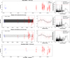 |
Fig. 1 Radial velocity (RV) analysis of GJ 4274. The top row shows the raw RV data with offsets removed (RMS = 7.06 m/s). The second and third rows display the contributions of planets b and c to the RV signal, respectively, along with their phase-folded RV curves. The RV data in the left panel for planet c are the residuals of the contribution of planet b. The bottom panel presents the residuals after removing all modeled signals (RMS = 5.20 m/s). The rightmost column contains the periodograms, which highlight significant periods in the RV data at each step. The significance level of FAP = 10−3 is indicated by the horizontal dashed red line. |
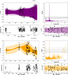 |
Fig. 2 Time series, periodograms, and Gaussian process (GP) regression fits for the activity indicators Bℓ (upper panel) and dTemp (lower panel). Each panel is divided into four subpanels. The upper-left subpanel shows the time series of this indicator (black dots), along with its GP fit (colored lines). The same, focused on the 2023 observations, are shown in the lower-right subpanel. The residuals of these fits are in the bottom subpanel. The upper-right subpanel displays the Lomb-Scargle periodogram of the activity indicator. In these subpanels, the vertical dashed blue line marks the known rotation periods of GJ 4274 (Prot = 4.59 d). The horizontal black lines (solid, dashed, and dotted) indicate false alarm probabilities (FAPs) of 10%, 1%, and 0.1%, respectively. |
4 Analysis of radial velocities
4.1 Detection of planetary signals
To search for planetary signals in the post-processed RV time series displayed in Fig. 1, we sequentially added significant signals to the model and recomputed the LS periodogram at each step. After the wapiti correction of systematics, the peri-odogram shows several peaks with a false alarm probability (FAP; Baluev 2008) less than 0.1% (i.e., above the dashed horizontal line in the right panel of Fig. 1). None of the peaks correspond to the rotation period of the star, nor to yearly harmonics. The strongest peak in the periodogram appears for a modulation period of 1.634 d with log FAP = –14.9. The one-day alias of this peak also appears at a measured period of 2.560 d (log FAP = –9.3). Initially, a planetary signal was added with the period of the strongest signal as a signal. We find that its fit eccentricity is consistent with 0 ( ), as expected from tidal interactions so close to the star. We then adopted a circular model (∆ log BF = 4.9 in favor of the circular model) because it was statistically more significant and more efficient to use due to the lower number of parameters. After adding the circular model of this planet, the strongest signal in the periodogram is for a period of 69.2 d (log FAP = –15.0), which was already visible in the initial RV data as the second strongest peak. This signal was added to the model, still assuming a circular orbit. Allowing eccentricity to vary again led to a null value and reduced statistical significance (∆ log BF = 8.5). After adding both signals, no significant signal remains above the detection threshold. We therefore fitted the two planets with circular orbits, using RadVel (Fulton et al. 2018) to perform an MCMC analysis, with 50 walkers, 2000 burn-in steps, and 10 000 subsequent steps. The priors and posterior distributions are displayed in Table 3, with the results of the two circular orbiting planets shown in the fourth column.
The MCMC analysis converges to RV planetary signatures with semi-amplitudes of  and 4.11 0.64 m/s for planets b and c, respectively, and orbital periods of 1.6339 ± 0.0001 and
  . These signals correspond to planetary companions with minimum masses of
  and
and  , using the stellar mass provided by Shan et al. (2024) (0.18 ± 0.02M⊙). The final RMS of the residuals is 5.20 m/s while the original RMS is 7.06 m/s. The dispersion of the residuals remains quite high compared to the precision of both instruments (∼ 1.9 m/s). No periodic signature of stellar activity is detected in the RV. The complete model is represented in Figure 1.
GP prior and fit parameters for GJ 4274 activity indicators Bℓ & dTemp.
4.2 The absence of activity signature in infrared RV data
At no step during this analysis was a signal detected that could correspond to magnetic activity, despite a clear modulation of the activity indicators (see Section 3), particularly Bℓ. This behavior in the SPIRou spectra is shared with several active M dwarfs (AD Leo, Carmona et al. 2023; DS Leo, Carmona et al. 2025; and EV Lac, Larue et al. 2025). We performed a multivariate GP analysis over the RVs with dTemp as the activity indicator (using pyaneti5 by Barragán et al. 2022). This resulted in weak GP amplitudes in the RV. This analysis is provided in Appendix C.
Larue et al. (2025) explored the nearly absence of an activity signature in RV from nIR spectroscopic data, despite the intense activity of active M dwarfs. In their recent study, they investigated how stellar spots affect different spectral lines. They identify two opposing regimes: in some lines, the spot produces a local absorption deficit, while in others, where the absorption of a chemical element is much stronger at the spot’s temperature than in the photosphere, it produces an absorption excess at the spot’s velocity. They also define a line-by-line spot-to-photosphere contrast, C. For EV Lac, the distribution of this contrast is well balanced around the neutral contrast C=1 in the SPIRou nIR domain, effectively canceling out when integrated over the full spectral range. Since GJ 4274 has a similar spectral type and rotational period to EV Lac, we suggest that the same phenomenon may also occur in this system. To assess this claim, we conducted a similar analysis. We find that the distribution of C is also well balanced around the neutral contrast C=1 over the entire SPIRou spectral range. Figure 3 shows the per-line contrast distribution. Furthermore, once identified, one can subtract the RV series derived from the lines with C>1 from the RV series derived from lines with C<1. This procedure combines the two contributions from the activity instead of canceling each other out, while canceling the planetary signals. This diagnosis will be explored and detailed further in future work. In the periodogram of this new indicator (Fig. 4), the rotation period emerges above the FAP 0.1% threshold, as does its 1d alias at 1.27 d, an alias that is also present in dTemp. The signals identified as planets do not appear in this indicator because they are present over all the lines and are not linked to the activity.
4.3 Alias analysis
In our analysis of the radial velocities of GJ 4274, we assumed that the 1.6339 d and 69.57 d periods represented the true orbital periods of the planets, as they corresponded to the largest peaks in the LS periodogram. However, as previously mentioned, numerous aliases of these periods are present with high significance. We conducted an alias analysis to determine the true orbital periods of the planets. We based our analysis on Dawson & Fabrycky (2010) and performed injection recovery tests. We first assumed that the largest peak represented the true period. We added this signal to the model and plotted its periodogram. We repeated the operation assuming that the other period represented the true period and compared the amplitudes and phases of the alias peaks in their periodograms. We also compared these to the predicted aliases given the window function.
Following this protocol, we compared different orbital solutions to the RV data. The resulting periodograms are shown in Figure 5. Initially, we compared the different models for the inner planet period, 1.6339 d and its one-day alias at 2.5598 d (panel b and c in Figure 5, respectively). The other 1 d alias at 0.62 d is not significant in the RV data. We find that the 1.6339 d model is more likely with ∆BF = 2.11. Comparing the model periodograms shows that they mainly differ in the order of the three first peaks. In the 1.6339 d model, the strongest peak corresponds to the 1.6339 d signal, followed by its alias at 2.5598 d, and thirdly the second planet at 69.57 d. In the 2.5598 d model, the 1.6339 d peak is weaker than the 2.5598 d signal, which is the dominant peak. The phases of the 1.6339 d and 2.5598 d signals match the 1.6339 d model better than the 2.5598 d model, as indicated by the dials. Dawson & Fabrycky (2010), citing Lomb (1976), concluded that “If there is a satisfactory match between an observed spectrum and a noise-free spectrum of period P, then P is the true period”. Furthermore, in the stacked periodogram shown in Figure 6 (Mortier & Collier Cameron 2017), the 1.6339 d signal always exhibits higher significance than the 2.5598 d signal, regardless of the number of observations. Both analyses using Bayesian statistics, Dawson & Fabrycky (2010) alias analysis, and stacked periodograms, provide substantial evidence that 1.6339 d is the true orbital period of the inner planet.
The outer planetary signal at 69.6 d also exhibits numerous aliases. The strongest is the one-year alias at 58.8 d, which is the only remaining alias with an FAP < 0.1% after fitting the first planet. We repeated the same analysis for these two periods (panel b and d in Figure 5). We find that the 69.6 d model is more likely, with ∆BF = 3.16. In the 58.8 d periodogram (panel d in Figure 5), the periodic signals produced by this modeled planet are much weaker than those in the RV data, particularly for the 69.6 d period. We conclude that the outer plane has a period of 69.6 d.
Fitted orbital parameters of GJ 4274 planet(s).
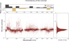 |
Fig. 3 Contrast computed for each line and their histograms. As defined by Larue et al. (2025), the neutral contrast C=1 is highlighted by the dotted lines. |
 |
Fig. 4 Periodogram of RV time series computed from lines with contrast C>1 (Fig. 3) subtracted from lines with C<1 (Fig. 3). |
4.4 CARMENES data
The limited number of CARMENES measurements, particularly after we removed the outliers, did not allow us to detect any periodic signals, nor any signals in their derived activity indicators, using only these data. Injection-recovery tests on these data show that no planetary signal could be confidently detected for planets with minimum masses below ~70 M⊕ for periods <100 d. However, the few data points we collected agree with the model derived using only SPIRou data. Furthermore, adding the CARMENES measurements reinforces the significance of the planetary signals in the periodogram, while relatively lowering their one-day alias counterpart (∆ log FAP(1.6339 d) = −2.4; ∆ log FAP(69.57 d) = −0.7; and ∆ log FAP(2.56 d) = +1.6). Thus, the joint use of both datasets reinforces our analysis. The CARMENES measurements are included in Fig. 1 as blue dots.
5 Discussion
5.1 Detectability of additional companions
The detection of two planets orbiting GJ 4274 does not imply that they are the only planets hosted by this star. The quality of the data, the observation strategy, atmospheric conditions, and stellar jitter all affect our detection sensitivity. We performed injection-recovery tests on the residuals of the previous model to assess detection sensitivity. For each cell in a grid of orbital period (1–3000 days, logarithmically spaced in 500 bins) and semi-amplitude (2–6 m/s, linearly spaced in 120 bins), we injected a sinusoidal signal, assuming a small eccentricity, consistent with most dwarf M planets, with a random phase. We then computed the LS periodogram and evaluated the FAP at the injected period. This procedure was repeated ten times for each period-amplitude input and averaged. The results of this procedure are shown in Figure 7.
Our injection–recovery tests show that no additional planetary companion inducing a radial velocity semi-amplitude below 3.5 m/s can be confidently detected with a FAP < 1% for periods between nine and 39 days, corresponding to the optimistic boundaries of the habitable zone (Kopparapu et al. 2013, 2014). For signals with a FAP < 0.1%, the upper limit on the semi-amplitude is 4 m/s. However, above 4 m/s, injected signals are reliably recovered, indicating that no additional companion inducing RV variations larger than this limit is likely present. In terms of minimum mass, this means that any undetected planet in the habitable zone of GJ 4274 would have a mass below M sin i = 4–7 M⊕, depending on its localization.
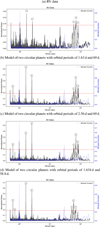 |
Fig. 5 Lomb–Scargle periodograms of RV data (top panel, identical to the first row of Fig. 1) and the modeled two circular planets’ RV signals. The planet periods are 1.63 d and 69.3 d (panel b), 2.56 d and 69.6 d (panel c), and 1.63 d and 58.8 d (panel d). Significant peaks are highlighted with phase-indicating dials. The vertical dashed red line represents the detectability limit (FAP < 0.1%). The window function is plotted in blue. |
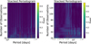 |
Fig. 6 Stacked periodograms of GJ 4274 RV data. The vertical red segments indicate the periodicities of the planets (longer segments) and their aliases (shorter segments). |
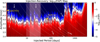 |
Fig. 7 Detection limits as a function of period and amplitude from injection-recovery tests. The orbital periods corresponding to both conservative and optimistic habitable zones (Kopparapu et al. 2013, 2014) are highlighted in pink. |
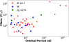 |
Fig. 8 Mass (M sin i) and period of confirmed exoplanets orbiting late-type stars within 15 pc. Planets from the same system are connected by colored lines. |
5.2 Comparison with other nearby systems
The GJ 4274 system resembles most planetary systems of late-type stars in the solar neighborhood but exhibits a few notable characteristics. To highlight these characteristics, we sampled all confirmed planets within 15 pc orbiting M dwarfs with masses below 0.2 M⊙. Some of their characteristics are shown in Figure 8. We extracted their properties from the NASA Exoplanet Archive6.
Firstly, we find that GJ 4274 b has one of the shortest orbital periods in the sample and the shortest discovered using only RVs. In our limited sample, only three planets orbited closer than GJ 4274 b, namely, TRAPPIST-1 b (1.510826 ± 0.000006 d, Agol et al. 2021), GJ 1214 b (1.580404531 ±0.00000018, Mahajan et al. 2024),and GJ 1132 b (1.62892911 ± 0.0000003, Xue et al. 2024).
Conversely, the orbital period of GJ 4274 c falls into a gap in the distribution that connects numerous close-in low-mass planets (<10M⊕) to the fewer, more distant giant planets beyond the snowline, calculated at 79.3 ± 6.6 d, using GJ 4274 stellar parameters. With a period of  and a semi-axis of 0.187 ± 0.002 a.u., GJ 4274c lies close to the outer limit of the habitable zone around GJ 4274. The CARMENES catalog (Cifuentes et al. 2020), provides the luminosity of this star, based on a compilation of photometric measurements, the GAIA DR2 catalog, and the BT-Settl CIFIST grid of models (Husser et al. 2013). Based on this value, the stellar flux received by GJ 4274c is approximately 10% of that received by Earth. Ramirez & Kaltenegger (2017, 2018) investigated the evolution of the habitable zone’s outer boundary as a function of atmospheric composition using 1D climate models, concluding that for M dwarfs with effective temperatures similar to GJ 4274, the outer edge for a canonical N2–CO2–H2O atmosphere lies near 0.23 S⊕. This limit shifts below 0.15 S⊕ (close to the insolation of GJ 4274c) for an atmosphere enriched with 50% H2 (e.g., from volcanic outgassing). Considering the limitations of 1D models in defining habitable zone boundaries, future theoretical studies should more precisely assess the habitability potential of a planet such as GJ 4274c. These limits are derived for Earth-like planets; however, the mass of GJ 4274c places it in the transition region of the mass–radius diagram, where sequences of terrestrial planets and mini-Neptunes overlap (Cloutier & Menou 2020). If GJ 4274c is a mini-Neptune with a significant H2 envelope, it therefore seems unlikely that such an atmosphere, with its strong greenhouse effect, could efficiently dissipate Neptune-like internal energy, particularly at such a young age. The temperature under the atmosphere is thus expected to be very high.
The GJ 4274 system is also consistent with global trends for these kinds of systems, including the global mass-period correlation, the increased multiplicity rate, and the small planet rate around such low-mass star.
5.3 Transit detectability with TESS
The close vicinity of the planets, especially the inner one, increases the transit probability. The derived parameters suggest a transit probability of ∼6% for planet b. However, we can rule out any transit event in the TESS photometric data. For the outer planet, the TESS photometric data do not cover the entire orbital phase, and no transit event is visible. The phase-folded TESS photometric data are available in Appendix in Figure A.1.
To assess transit detectability of planet b, we performed an injection-recovery test on the TESS light curve, simulating transits over grids of orbital inclinations and planetary radii using the batman package (Kreidberg 2015), following the protocol developed by Cortés-Zuleta et al. (2025). Inclinations ranged from 86° to 73° in bins of 0.1°, while radii ranged from 1 to 4 R⊕ in bins of 0.1 R⊕. The radial range is motivated by radius distributions found with spright (Parviainen et al. 2024), using empirical mass-radius relationship based on the Small Transiting Planets around M dwarfs (STPM) catalog by Luque & Pallé (2022) and derived from the planets’ minimum masses. This distribution is shown in Figure 9. It ranges from 1.3 to 3.5 R⊕ for planet b and 1.8 to 4.9 R⊕ for planet c, within the 95% confidence interval, with median values of 1.47 and 2.85 R⊕, respectively. We adopted the limb darkening coefficients from Table 15 in Claret (2017). We then applied the box least square (BLS; Kovács et al. 2002) periodogram to test detection, considering a signal detectable when the FAP, determined by bootstrapping, was below 0.1%. The results, displayed in Figure 10, show that planet b would have been detected if its radius exceeded 1.3 R⊕ and its inclination was greater than 83°, implying that its actual inclination is lower. In a perfectly edge-on configuration, even a 0.2 R⊕ planet would have been detectable, but such an object with the measured mass would be unrealistically dense. For planet c, the detection is ambiguous because of the limited phase coverage, but if its orbit is aligned with that of planet b, it likely does not transit.
This analysis supports the conclusions drawn from activity indicators. The large amplitude range and regular sign switch of the longitudinal magnetic field (±200 G) suggest a relatively high inclination of the stellar spin axis from the line of sight (typically around 60°, as observed for EV Lac, Morin et al. 2008). We therefore conclude that GJ 4274 is a non-transiting planetary system.
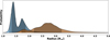 |
Fig. 9 Probability density distribution of the predicted planet radius of GJ 4274 b (blue) and c (brown) obtained using spright. |
 |
Fig. 10 Detectability of planet b transit in TESS light curves of GJ 4274 versus orbital inclination and planetary radius. Colors indicate the detection probability, as described in Sect. 5.3. The shaded gray area shows the predicted radius range corresponding to the planet minimum mass, with the darkest shade representing the 64% confidence interval and the lightest shade the 95% interval. The vertical gray line marks the median value derived using spright. |
5.4 Prospect for future instruments
The absence of transit does not rule-out follow-up observations to characterize their atmosphere. The proximity of GJ4274 (7.2344 ± 0.0025 pc) implies a favorable projected separation (25.72 ± 0.28 mas) for planet c. It would be possible through reflected spectroscopy using next generation spectrographs such as ANDES (Palle et al. 2025), providing a challenging target for that instrument. From the derived planetary parameters, we estimate a planet-star contrast between 1–6 × 10⁻⁸, depending on the assumed albedo. Given the star’s magnitude, the atmosphere of planet c might be detected within a few hours under the most favorable conditions.
The system’s proximity also implies a favorable projected astrometric signature. From the derived planetary parameters, we compute that the projected semi-major axis of the stellar reflex motion is  for planet c. However, at this stellar magnitude, Gaia end-of-mission precision is on the order of a few 10 µas (Gaia Collaboration 2023). Therefore, GJ 4274 planets would not be detectable by Gaia astrometry. Future projects, such as ESA’s Theia mission (The Theia Collaboration 2017), which aims to surpass the µas barrier, might be able to observe GJ 4274 c. Such observations would definitively confirm the planet’s existence and constrain the system’s inclination, thereby determining the true planetary masses.
6 Conclusions
We report the discovery of two exoplanets around the nearby M dwarf star GJ 4274 periods of Pb = 1.6339 ± 0.0001 and  , respectively. From their RV semi-amplitude signals, we derive minimum masses of mb sin i = 2.99 ± 0.40 M⊕ for planet b and mc sin i = 8.41 ± 1.32 M⊕ for planet c. This discovery was achieved with the SPIRou high-precision nIR spectrograph as part of the SLS and SPICE large programs.
From the activity indicators Bℓ and dTemp, we derive a stellar rotation period of  , consistent with previous estimates of Newton et al. (2018) and Shan et al. (2024). Despite the intensity measured in these indicators, stellar activity does not significantly impact the nIR RV data. The stellar activity signature appears to be suppressed in the nIR bands due to stellar spot-to-photosphere contrast and anti-contrast effects canceling each other out, as demonstrated by Larue et al. (2025) for the similarly magnetically active M dwarf EV Lac.
The close proximity of the planets to their host star, especially the inner one, provides a relatively high transit probability of 5.75%. However, the analysis of TESS photometric data shows no transit for the inner planet and the photometric data do not fully cover the orbital phase of planet c). Injection-recovery tests allowed us to constrain an upper limit on the inclination of planet b of ib ≤ 83°.
The GJ 4274 system shares many characteristics with other planetary systems around late-type, low-mass M dwarfs, yet it also presents notable distinctions. GJ 4274 b has one of the shortest orbital periods among planets orbiting stars less massive than 0.2 M⊙ within 15 pc, and is the shortest-period planet in this category detected solely through RVs. GJ 4274 c lies in a sparsely populated region of the mass–period diagram, between numerous close-in low-mass planets (<10 M⊕) and the more distant giant planets beyond the snow line. These planets likely belong to the super-Earth or sub-Neptune classes, reinforcing known trends such as the mass–period correlation and high occurrence rates of small planets around very low-mass stars. Their discovery enriches the census of nearby planetary systems and provides challenging targets for atmospheric characterization, with the angular separation of GJ 4274 c making it particularly accessible to future spatially resolved high-resolution spectroscopy with instruments such as ANDES.
Data availability
The data used in this work were were collected as part of the SPIRou Legacy Survey (SLS) and the SPICE large program, and they became publicly available at the Canadian Astronomy Data Center7 (CADC) one year after completion of the program, i.e., since February 2024 for SLS data and August 2025 for the SPICE data.
The RV, Bℓ and dTemp time-series used for this paper are available at the Strasbourg astronomical Data Center (CDS) via https://cdsarc.cds.unistra.fr/viz-bin/cat/J/A+A/705/A243.
Acknowledgements
This project received funding from the European Research Council (ERC) under the H2020 research & innovation program (grant #740651 NewWorlds). Our work is based on observations obtained at the Canada–France–Hawaii Telescope (CFHT), which is operated by the National Research Council (NRC) of Canada, the Institut National des Sciences de l’Univers of the Centre National de la Recherche Scientifique (INSU/CNRS) of France, and the University of Hawaii. The CFHT observations were performed with great care and respect from the summit of Maunakea, a location of immense cultural and historical significance. We wish to acknowledge the significant cultural role and reverence that the summit of Maunakea has always held within the indigenous Hawaiian community. We are incredibly fortunate to have had the opportunity to conduct observations from this mountain, which plays a vital part in our study. X.D. acknowledge funding from the French ANR under contract number ANR-24-CE49-3397 (ORVET), and the French National Research Agency in the framework of the Investissements d’Avenir program (ANR-15-IDEX-02), through the funding of the “Origin of Life” project of the Grenoble-Alpes University. E.A., C.C., A.L’H., and N.J.C. acknowledge the financial support of the FRQ-NT through the Centre de recherche en astro-physique du Québec, as well as the support from the Trottier Family Foundation and the Trottier Institute for Research on Exoplanets.
References
- Agol, E., Dorn, C., Grimm, S. L., et al. 2021, Planet. Sci. J., 2, 1 [NASA ADS] [CrossRef] [Google Scholar]
- Aigrain, S., Pont, F., & Zucker, S. 2012, MNRAS, 419, 3147 [NASA ADS] [CrossRef] [Google Scholar]
- Andersen, J. M., & Korhonen, H. 2015, MNRAS, 448, 3053 [NASA ADS] [CrossRef] [Google Scholar]
- Anglada-Escudé, G., Amado, P. J., Barnes, J., et al. 2016, Nature, 536, 437 [Google Scholar]
- Artigau, É., Cadieux, C., Cook, N. J., et al. 2022, AJ, 164, 84 [NASA ADS] [CrossRef] [Google Scholar]
- Artigau, É., Bouchy, F., Doyon, R., et al. 2024a, SPIE Conf. Ser., 13096, 130960C [Google Scholar]
- Artigau, É., Cadieux, C., Cook, N. J., et al. 2024b, AJ, 168, 252 [Google Scholar]
- Baluev, R. V. 2008, MNRAS, 385, 1279 [Google Scholar]
- Barragán, O., Aigrain, S., Rajpaul, V. M., & Zicher, N. 2022, MNRAS, 509, 866 [Google Scholar]
- Basant, R., Luque, R., Bean, J. L., et al. 2025, ApJ, 982, L1 [Google Scholar]
- Bertaux, J. L., Lallement, R., Ferron, S., Boonne, C., & Bodichon, R. 2014, A&A, 564, A46 [NASA ADS] [CrossRef] [EDP Sciences] [Google Scholar]
- Bonfils, X., Delfosse, X., Udry, S., et al. 2013, A&A, 549, A109 [NASA ADS] [CrossRef] [EDP Sciences] [Google Scholar]
- Bortle, A., Fausey, H., Ji, J., et al. 2021, AJ, 161, 230 [NASA ADS] [CrossRef] [Google Scholar]
- Bouchy, F., Pepe, F., & Queloz, D. 2001, A&A, 374, 733 [NASA ADS] [CrossRef] [EDP Sciences] [Google Scholar]
- Bouchy, F., Díaz, R. F., Hébrard, G., et al. 2013, A&A, 549, A49 [NASA ADS] [CrossRef] [EDP Sciences] [Google Scholar]
- Bouchy, F., Doyon, R., Pepe, F., et al. 2025, A&A, 700, A10 [NASA ADS] [CrossRef] [EDP Sciences] [Google Scholar]
- Burn, R., Schlecker, M., Mordasini, C., et al. 2021, A&A, 656, A72 [NASA ADS] [CrossRef] [EDP Sciences] [Google Scholar]
- Cale, B. L., Reefe, M., Plavchan, P., et al. 2021, AJ, 162, 295 [NASA ADS] [CrossRef] [Google Scholar]
- Camacho, J. D., Faria, J. P., & Viana, P. T. P. 2023, MNRAS, 519, 5439 [NASA ADS] [CrossRef] [Google Scholar]
- Carleo, I., Malavolta, L., Lanza, A. F., et al. 2020, A&A, 638, A5 [NASA ADS] [CrossRef] [EDP Sciences] [Google Scholar]
- Carmona, A., Delfosse, X., Bellotti, S., et al. 2023, A&A, 674, A110 [NASA ADS] [CrossRef] [EDP Sciences] [Google Scholar]
- Carmona, A., Delfosse, X., Ould-Elhkim, M., et al. 2025, A&A, 700, A222 [NASA ADS] [CrossRef] [EDP Sciences] [Google Scholar]
- Chabrier, G., & Baraffe, I. 1997, A&A, 327, 1039 [NASA ADS] [Google Scholar]
- Cifuentes, C., Caballero, J. A., Cortés-Contreras, M., et al. 2020, A&A, 642, A115 [NASA ADS] [CrossRef] [EDP Sciences] [Google Scholar]
- Claret, A. 2017, A&A, 600, A30 [NASA ADS] [CrossRef] [EDP Sciences] [Google Scholar]
- Cloutier, R., & Menou, K. 2020, AJ, 159, 211 [NASA ADS] [CrossRef] [Google Scholar]
- Cook, N. J., Artigau, É, Doyon, R., et al. 2022, PASP, 134, 114509 [NASA ADS] [CrossRef] [Google Scholar]
- Cortés-Zuleta, P., Boisse, I., Ould-Elhkim, M., et al. 2025, A&A, 693, A164 [NASA ADS] [CrossRef] [EDP Sciences] [Google Scholar]
- Cretignier, M., Dumusque, X., Allart, R., Pepe, F., & Lovis, C. 2020, A&A, 633, A76 [NASA ADS] [CrossRef] [EDP Sciences] [Google Scholar]
- Dawson, R. I., & Fabrycky, D. C. 2010, ApJ, 722, 937 [Google Scholar]
- Delchambre, L. 2015, MNRAS, 446, 3545 [NASA ADS] [CrossRef] [Google Scholar]
- Desort, M., Lagrange, A. M., Galland, F., Udry, S., & Mayor, M. 2007, A&A, 473, 983 [CrossRef] [EDP Sciences] [Google Scholar]
- Donati, I.-F., Kouach, D., Moutou, C., et al. 2020, MNRAS, 498, 5684 [NASA ADS] [CrossRef] [Google Scholar]
- Donati, J. F., Semel, M., Carter, B. D., Rees, D. E., & Collier Cameron, A. 1997, MNRAS, 291, 658 [Google Scholar]
- Dumusque, X. 2018, A&A, 620, A47 [NASA ADS] [CrossRef] [EDP Sciences] [Google Scholar]
- Faria, J. P., Suárez Mascareño, A., Figueira, P., et al. 2022, A&A, 658, A115 [NASA ADS] [CrossRef] [EDP Sciences] [Google Scholar]
- Fischer, D. A., Anglada-Escude, G., Arriagada, P., et al. 2016, PASP, 128, 066001 [Google Scholar]
- Foreman-Mackey, D., Hogg, D. W., Lang, D., & Goodman, J. 2013, PASP, 125, 306 [Google Scholar]
- Fulton, B. J., Petigura, E. A., Blunt, S., & Sinukoff, E. 2018, PASP, 130, 044504 [Google Scholar]
- Gaia Collaboration 2020, VizieR Online Data Catalog: Gaia EDR3 (Gaia Collaboration, 2020), VizieR On-line Data Catalog: I/350. Originally published in: 2021A & A…649A…1G [Google Scholar]
- Gaia Collaboration (Vallenari, A., et al.) 2023, A&A, 674, A1 [NASA ADS] [CrossRef] [EDP Sciences] [Google Scholar]
- González Hernández, J. I., Suárez Mascareño, A., Silva, A. M., et al. 2024, A&A, 690, A79 [NASA ADS] [CrossRef] [EDP Sciences] [Google Scholar]
- Haywood, R. D., Collier Cameron, A., Queloz, D., et al. 2014, MNRAS, 443, 2517 [Google Scholar]
- Henry, T. J., Jao, W.-C., Subasavage, J. P., et al. 2006, AJ, 132, 2360 [Google Scholar]
- Hobson, M. J., Bouchy, F., Cook, N. J., et al. 2021, A&A, 648, A48 [NASA ADS] [CrossRef] [EDP Sciences] [Google Scholar]
- Huélamo, N., Figueira, P., Bonfils, X., et al. 2008, A&A, 489, L9 [NASA ADS] [CrossRef] [EDP Sciences] [Google Scholar]
- Husser, T. O., Wende-von Berg, S., Dreizler, S., et al. 2013, A&A, 553, A6 [NASA ADS] [CrossRef] [EDP Sciences] [Google Scholar]
- Kanodia, S., & Wright, J. 2018, RNAAS, 2, 4 [NASA ADS] [Google Scholar]
- Kochukhov, O. 2021, A&A Rev., 29, 1 [NASA ADS] [CrossRef] [Google Scholar]
- Kopparapu, R. K., Ramirez, R., Kasting, J. F., et al. 2013, ApJ, 765, 131 [NASA ADS] [CrossRef] [Google Scholar]
- Kopparapu, R. K., Ramirez, R. M., SchottelKotte, J., et al. 2014, ApJ, 787, L29 [Google Scholar]
- Kotani, T., Tamura, M., Suto, H., et al. 2014, SPIE Conf. Ser., 9147, 914714 [NASA ADS] [Google Scholar]
- Kovács, G., Zucker, S., & Mazeh, T. 2002, A&A, 391, 369 [Google Scholar]
- Kreidberg, L. 2015, PASP, 127, 1161 [Google Scholar]
- Kurucz, R. L. 1992, in IAU Symposium, 149, The Stellar Populations of Galaxies, eds. B. Barbuy, & A. Renzini, 225 [Google Scholar]
- Lagrange, A. M., Meunier, N., Desort, M., & Malbet, F. 2011, A&A, 528, L9 [NASA ADS] [CrossRef] [EDP Sciences] [Google Scholar]
- Larue, P., Delfosse, X., Carmona, A., et al. 2025, A&A [Google Scholar]
- Lehmann, L. T., Donati, J. F., Fouqué, P., et al. 2024, MNRAS, 527, 4330 [Google Scholar]
- Lightkurve Collaboration (Cardoso, J. V. d. M., et al.) 2018, Astrophysics Source Code Library [record ascl:1812.013] [Google Scholar]
- Lomb, N. R. 1976, Ap & SS, 39, 447 [NASA ADS] [CrossRef] [Google Scholar]
- Luque, R., & Pallé, E. 2022, Science, 377, 1211 [NASA ADS] [CrossRef] [Google Scholar]
- Mahadevan, S., Ramsey, L., Bender, C., et al. 2012, SPIE Conf. Ser., 8446, 84461S [NASA ADS] [Google Scholar]
- Mahajan, A. S., Eastman, J. D., & Kirk, J. 2024, ApJ, 963, L37 [NASA ADS] [CrossRef] [Google Scholar]
- Mahmud, N. I., Crockett, C. J., Johns-Krull, C. M., et al. 2011, ApJ, 736, 123 [NASA ADS] [CrossRef] [Google Scholar]
- Marfil, E., Tabernero, H. M., Montes, D., et al. 2021, A&A, 656, A162 [NASA ADS] [CrossRef] [EDP Sciences] [Google Scholar]
- Martín, E. L., Guenther, E., Zapatero Osorio, M. R., Bouy, H., & Wainscoat, R. 2006, ApJ, 644, L75 [CrossRef] [Google Scholar]
- Mayor, M., & Queloz, D. 1995, Nature, 378, 355 [Google Scholar]
- Meunier, N., & Lagrange, A. M. 2019, A&A, 625, L6 [NASA ADS] [CrossRef] [EDP Sciences] [Google Scholar]
- Meunier, N., Desort, M., & Lagrange, A. M. 2010, A&A, 512, A39 [NASA ADS] [CrossRef] [EDP Sciences] [Google Scholar]
- Mignon, L., Delfosse, X., Meunier, N., et al. 2025, A&A, 700, A146 [NASA ADS] [CrossRef] [EDP Sciences] [Google Scholar]
- Morin, J., Donati, J. F., Petit, P., et al. 2008, MNRAS, 390, 567 [Google Scholar]
- Morin, J., Donati, J. F., Petit, P., et al. 2010, MNRAS, 407, 2269 [Google Scholar]
- Mortier, A., & Collier Cameron, A. 2017, A&A, 601, A110 [NASA ADS] [CrossRef] [EDP Sciences] [Google Scholar]
- Moutou, C., Delfosse, X., Petit, A. C., et al. 2023, A&A, 678, A207 [NASA ADS] [CrossRef] [EDP Sciences] [Google Scholar]
- Newton, E. R., Mondrik, N., Irwin, J., Winters, J. G., & Charbonneau, D. 2018, AJ, 156, 217 [Google Scholar]
- Ould-Elhkim, M., Moutou, C., Donati, J.-F., et al. 2023, A&A, 675, A187 [NASA ADS] [CrossRef] [EDP Sciences] [Google Scholar]
- Palle, E., Biazzo, K., Bolmont, E., et al. 2025, Exp. Astron., 59, 29 [Google Scholar]
- Parviainen, H., Luque, R., & Palle, E. 2024, MNRAS, 527, 5693 [Google Scholar]
- Pepe, F., Cristiani, S., Rebolo, R., et al. 2021, A&A, 645, A96 [NASA ADS] [CrossRef] [EDP Sciences] [Google Scholar]
- Pinamonti, M., Sozzetti, A., Maldonado, J., et al. 2022, A&A, 664, A65 [NASA ADS] [CrossRef] [EDP Sciences] [Google Scholar]
- Quirrenbach, A., Amado, P. J., Ribas, I., et al. 2018, SPIE Conf. Ser., 10702, 107020 W [NASA ADS] [Google Scholar]
- Rajpaul, V., Aigrain, S., Osborne, M. A., Reece, S., & Roberts, S. 2015, MNRAS, 452, 2269 [Google Scholar]
- Ramirez, R. M., & Kaltenegger, L. 2017, ApJ, 837, L4 [Google Scholar]
- Ramirez, R. M., & Kaltenegger, L. 2018, ApJ, 858, 72 [Google Scholar]
- Reiners, A. 2009, A&A, 498, 853 [NASA ADS] [CrossRef] [EDP Sciences] [Google Scholar]
- Reiners, A., Bean, J. L., Huber, K. F., et al. 2010, ApJ, 710, 432 [Google Scholar]
- Reiners, A., Shulyak, D., Anglada-Escudé, G., et al. 2013, A&A, 552, A103 [NASA ADS] [CrossRef] [EDP Sciences] [Google Scholar]
- Reylé, C., Jardine, K., Fouqué, P., et al. 2021, A&A, 650, A201 [Google Scholar]
- Ribas, I., Reiners, A., Zechmeister, M., et al. 2023, A&A, 670, A139 [NASA ADS] [CrossRef] [EDP Sciences] [Google Scholar]
- Ricker, G. R., Winn, J. N., Vanderspek, R., et al. 2015, J. Astron. Telesc. Instrum. Syst., 1, 014003 [Google Scholar]
- Robertson, P., Stefansson, G., Mahadevan, S., et al. 2020, ApJ, 897, 125 [NASA ADS] [CrossRef] [Google Scholar]
- Sabotta, S., Schlecker, M., Chaturvedi, P., et al. 2021, A&A, 653, A114 [NASA ADS] [CrossRef] [EDP Sciences] [Google Scholar]
- Schöfer, P., Jeffers, S. V., Reiners, A., et al. 2022, A&A, 663, A68 [NASA ADS] [CrossRef] [EDP Sciences] [Google Scholar]
- Seifahrt, A., Stürmer, J., Bean, J. L., & Schwab, C. 2018, SPIE Conf. Ser., 10702, 107026D [NASA ADS] [Google Scholar]
- Shan, Y., Revilla, D., Skrzypinski, S. L., et al. 2024, A&A, 684, A9 [NASA ADS] [CrossRef] [EDP Sciences] [Google Scholar]
- Stassun, K. G., Oelkers, R. J., Paegert, M., et al. 2019, AJ, 158, 138 [Google Scholar]
- Stock, S., Kemmer, J., Kossakowski, D., et al. 2023, A&A, 674, A108 [NASA ADS] [CrossRef] [EDP Sciences] [Google Scholar]
- The Theia Collaboration (Boehm, C., et al.) 2017, arXiv e-prints [arXiv:1707.01348] [Google Scholar]
- Xue, Q., Bean, J. L., Zhang, M., et al. 2024, ApJ, 973, L8 [NASA ADS] [CrossRef] [Google Scholar]
- Zechmeister, M., Reiners, A., Amado, P. J., et al. 2018, A&A 609 A12 [NASA ADS] [CrossRef] [EDP Sciences] [Google Scholar]
Under the runs 20AP40, 22AP40, 23AP45, 23BP45, 24AP45 (PI: J.-F. Donati), and 24BC12 (PI: E. Artigau).
The wavelength calibration uses a combination of exposures from a uranium–neon (UNe) hollow cathode lamp and a Fabry-Pérot etalon (Hobson et al. 2021).
Appendix A TESS photometric data
TESS photometric data are shown in figure A.1.
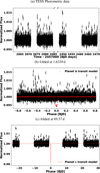 |
Fig. A.1 TESS photometric data folded on the derived periods of respectively the planet b (middle panel) and c (bottom panel). On the background of the two last panels is over plotted a transit model of the planets assuming i = 90° and taking the nominal value for all the other parameters. |
Appendix B Supplementary materials regarding MCMC analyses
Appendix B.1 Analysis of RV using radvel
The corner plot corresponding to the MCMC analysis presented in Section 4 is presented in Figure B.1.
Appendix B.2 Analysis of Bℓ
The corner plot corresponding to the MCMC analysis of the GP of the longitudinal magnetic field presented in Section 3 is presented in Figure B.2.
Appendix B.3 Analysis of dTemp
The corner plot corresponding to the MCMC analysis of the GP of the differential effective temperature presented in Section 3 is presented in Figure B.3.
Appendix C Multivariate GP
As mentioned in the main body of the article, we have tried to fit both the planets and the activity in the RV using a multivariate GP to train the GP with the activity indicator dTemp. dTemp is the indicator that best reflects the photometric flux (F), bringing us closer to the FF’ framework developed by Aigrain et al. (2012). We used the pyaneti8 implementation from Barragán et al. (2022) briefly described as follows:

with RV(t) the radial velocities measurements; AI(t) the measurements on the same time samples of one activity indicator (dTemp here); G the Gaussian Process defined with a quasiperiodic kernel with the covariance function described by equation 2 (with a fixed to 1), and G′ the derivative of that QP-GPR. This framework is similar to the one established by Rajpaul et al. (2015). The prior and posterior distributions are displayed in Table C.1. This analysis requires both the RV and the activity indicator to be on the same time sample, which excludes the RV data points from CARMENES. Since no periodic activity signal is visible in the RV, we had to hardly constrain some of the parameters to ensure the convergence. The derived parameters from this fit are compatible with both planetary parameters found in table 3 and GP hyper-parameters table 2.
Prior and posterior fits of a multivariate GP on RV and dTemp with 2 planets on circular orbits.
 |
Fig. B.1 Corner plot of the posterior distributions for planetary, instrumental, and systematics parameters, including instruments offsets, jitter terms and wapiti correction coefficients |
 |
Fig. B.2 Corner plot of the posterior distribution for the hyper-parameter fit of a QP-GP on the Bℓ indicator for the star GJ 4274 |
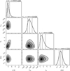 |
Fig. B.3 Corner plot of the posterior distribution for the hyper-parameter fit of a QP-GP on the dTemp indicator for the star GJ 4274 |
All Tables
Prior and posterior fits of a multivariate GP on RV and dTemp with 2 planets on circular orbits.
All Figures
|
Fig. 1 Radial velocity (RV) analysis of GJ 4274. The top row shows the raw RV data with offsets removed (RMS = 7.06 m/s). The second and third rows display the contributions of planets b and c to the RV signal, respectively, along with their phase-folded RV curves. The RV data in the left panel for planet c are the residuals of the contribution of planet b. The bottom panel presents the residuals after removing all modeled signals (RMS = 5.20 m/s). The rightmost column contains the periodograms, which highlight significant periods in the RV data at each step. The significance level of FAP = 10−3 is indicated by the horizontal dashed red line. |
| In the text | |
|
Fig. 2 Time series, periodograms, and Gaussian process (GP) regression fits for the activity indicators Bℓ (upper panel) and dTemp (lower panel). Each panel is divided into four subpanels. The upper-left subpanel shows the time series of this indicator (black dots), along with its GP fit (colored lines). The same, focused on the 2023 observations, are shown in the lower-right subpanel. The residuals of these fits are in the bottom subpanel. The upper-right subpanel displays the Lomb-Scargle periodogram of the activity indicator. In these subpanels, the vertical dashed blue line marks the known rotation periods of GJ 4274 (Prot = 4.59 d). The horizontal black lines (solid, dashed, and dotted) indicate false alarm probabilities (FAPs) of 10%, 1%, and 0.1%, respectively. |
| In the text | |
|
Fig. 3 Contrast computed for each line and their histograms. As defined by Larue et al. (2025), the neutral contrast C=1 is highlighted by the dotted lines. |
| In the text | |
|
Fig. 4 Periodogram of RV time series computed from lines with contrast C>1 (Fig. 3) subtracted from lines with C<1 (Fig. 3). |
| In the text | |
|
Fig. 5 Lomb–Scargle periodograms of RV data (top panel, identical to the first row of Fig. 1) and the modeled two circular planets’ RV signals. The planet periods are 1.63 d and 69.3 d (panel b), 2.56 d and 69.6 d (panel c), and 1.63 d and 58.8 d (panel d). Significant peaks are highlighted with phase-indicating dials. The vertical dashed red line represents the detectability limit (FAP < 0.1%). The window function is plotted in blue. |
| In the text | |
|
Fig. 6 Stacked periodograms of GJ 4274 RV data. The vertical red segments indicate the periodicities of the planets (longer segments) and their aliases (shorter segments). |
| In the text | |
|
Fig. 7 Detection limits as a function of period and amplitude from injection-recovery tests. The orbital periods corresponding to both conservative and optimistic habitable zones (Kopparapu et al. 2013, 2014) are highlighted in pink. |
| In the text | |
|
Fig. 8 Mass (M sin i) and period of confirmed exoplanets orbiting late-type stars within 15 pc. Planets from the same system are connected by colored lines. |
| In the text | |
|
Fig. 9 Probability density distribution of the predicted planet radius of GJ 4274 b (blue) and c (brown) obtained using spright. |
| In the text | |
|
Fig. 10 Detectability of planet b transit in TESS light curves of GJ 4274 versus orbital inclination and planetary radius. Colors indicate the detection probability, as described in Sect. 5.3. The shaded gray area shows the predicted radius range corresponding to the planet minimum mass, with the darkest shade representing the 64% confidence interval and the lightest shade the 95% interval. The vertical gray line marks the median value derived using spright. |
| In the text | |
|
Fig. A.1 TESS photometric data folded on the derived periods of respectively the planet b (middle panel) and c (bottom panel). On the background of the two last panels is over plotted a transit model of the planets assuming i = 90° and taking the nominal value for all the other parameters. |
| In the text | |
|
Fig. B.1 Corner plot of the posterior distributions for planetary, instrumental, and systematics parameters, including instruments offsets, jitter terms and wapiti correction coefficients |
| In the text | |
|
Fig. B.2 Corner plot of the posterior distribution for the hyper-parameter fit of a QP-GP on the Bℓ indicator for the star GJ 4274 |
| In the text | |
|
Fig. B.3 Corner plot of the posterior distribution for the hyper-parameter fit of a QP-GP on the dTemp indicator for the star GJ 4274 |
| In the text | |
Current usage metrics show cumulative count of Article Views (full-text article views including HTML views, PDF and ePub downloads, according to the available data) and Abstracts Views on Vision4Press platform.
Data correspond to usage on the plateform after 2015. The current usage metrics is available 48-96 hours after online publication and is updated daily on week days.
Initial download of the metrics may take a while.