| Issue |
A&A
Volume 705, January 2026
|
|
|---|---|---|
| Article Number | A239 | |
| Number of page(s) | 18 | |
| Section | Interstellar and circumstellar matter | |
| DOI | https://doi.org/10.1051/0004-6361/202557938 | |
| Published online | 27 January 2026 | |
Spiral excitation in protoplanetary disks through gap-edge illumination
Distinctive kinematic signatures in CO isotopologues
1
Max-Planck-Institut für Astronomie,
Königstuhl 17,
Heidelberg
69117,
Germany
2
Max-Planck-Institut für Astrophysik,
Karl-Schwarzschild-Straße 1,
Garching bei München
85748,
Germany
3
Institut für Theoretische Astrophysik, Ruprecht-Karls Universität Heidelberg,
Albert-Ueberle-Straße 2,
Heidelberg
69120,
Germany
★ Corresponding author: This email address is being protected from spambots. You need JavaScript enabled to view it.
; This email address is being protected from spambots. You need JavaScript enabled to view it.
Received:
2
November
2025
Accepted:
27
November
2025
Abstract
High-resolution near-infrared observations have revealed prominent two-armed spirals in a multitude of systems, such as MWC 758, SAO 206462, and V1247 Ori. Alongside the classical theory of disk–companion interaction, shadow-based driving has come into vogue as a potential explanation for such large-scale substructures. This raises the question of how these two mechanisms might be distinguished from one another in observations. To investigate this question, we ran a pair of hydrodynamical simulations with PLUTO. The first, with full radiation hydrodynamics and gas-grain collision, was designed to develop shadow-driven spirals at the outer gap edge of a subthermal Saturn-mass planet. The second simulation, with parameterized β-cooling, was set up to capture the more standard view of spiral wave excitation by a super-thermal, multi-Jupiter-mass, exterior planetary companion. Post-processing of these simulations with the Monte Carlo radiative transfer (MCRT) code RADMC3D revealed that strong vertical velocities in the shadow-driven case create a prominent two-armed feature in the moment-1 CO maps, particularly when the disk is viewed face-on in optically thicker isotopologues; this feature is not seen in the standard planet-driven case. Conversely, the presence or absence of such signatures in two-armed spiral systems would distinguish those potentially driven by exterior multi-Jupiter-mass companions, and thus help identify promising targets for future direct-imaging campaigns.
Key words: accretion / accretion disks / planet-disk interactions
© The Authors 2026
 Open Access article, published by EDP Sciences, under the terms of the Creative Commons Attribution License (https://creativecommons.org/licenses/by/4.0), which permits unrestricted use, distribution, and reproduction in any medium, provided the original work is properly cited.
This article is published in open access under the Subscribe to Open model.
Open Access funding provided by Max Planck Society.
1 Introduction
Detailed multiwavelength observations of circumstellar disks around forming stars – performed by instruments such as ALMA and VLT/SPHERE – have demonstrated that they contain a rich diversity of substructure, including gaps, rings (e.g., Andrews et al. 2018), and spirals (Teague et al. 2019, 2022) in their gas and dust components. The traditional explanation, which has been the subject of numerous analytical (e.g., Goldreich & Tremaine 1978, 1979, 1980) and numerical (Fung et al. 2014; Fung & Dong 2015; Zhu et al. 2015; Zhang et al. 2024) studies over the decades, is that such features result from gravitational interaction between the disk and nascent planetary companions: the spirals from the supersonic motion of the planetary potential through the disk gas, and the gaps and rings the cumulative result of angular momentum exchange through these spirals over thousands of planetary orbits. Among other mechanisms, such as photoevaporation (Ercolano & Picogna 2022), magnetohydrodynamical zonal flows (Hu et al. 2022), infalling material (Kuznetsova et al. 2022; Calcino et al. 2025), and gravitational instability (e.g., Dong et al. 2015a; Béthune et al. 2021), recent simulations (among others, the work of Montesinos et al. 2016; Montesinos & Cuello 2018; Su & Bai 2024), including some with full radiation hydrodynamics (e.g., Zhang & Zhu 2024; Ziampras et al. 2025), have demonstrated that the temperature variations created by shadows on the disk are also capable of driving substructure. Disk-shadow interaction follows an analytical theory that bears many similarities to that of disk-planet interaction (Zhu et al. 2025).
Of particular interest in this context are the various observed double-armed spirals in near-infrared (NIR) scattered light (e.g., Shuai et al. 2022), exemplified by systems such as MWC 758 (Grady et al. 2013), SAO 206462/HD 135344B (Muto et al. 2012), and V1247 Ori (Ren et al. 2024). According to the standard theory of disk-planet interaction, these two-armed spirals indicate the presence of an exterior multi-Jupiter-mass driver (Dong & Fung 2017; Bae & Zhu 2018a,b). In a companion paper to this work (Muley et al. 2024b), however, we demonstrate with 3D radiation-hydrodynamical simulations that shadowing effects at the outer edges of planet-carved gaps are also capable of driving large-scale two-armed spirals. For this alternative hypothesis, the minimum masses (Saturn- to Jupiter-mass) and semimajor axes (interior to the observed spirals rather than exterior) are far smaller than required classically.
Advances in NIR angular differential imaging (ADI; Asensio-Torres et al. 2021; Desidera et al. 2021), mid-infrared James Webb Space Telescope (JWST) MIRI (e.g., Wagner et al. 2019, 2024; Cugno et al. 2024), and spectroscopy of accretion tracers such as Hα and Paβ (Follette et al. 2023; Biddle et al. 2024) mean that the massive external companions predicted by the classical theory ought to be relatively accessible to observations. Despite putative detections (e.g., Wagner et al. 2023; Xie et al. 2024) and circumstantial support from spiral pattern speeds (e.g., Ren et al. 2018, 2020, 2024), conclusive evidence of such companions alongside two-armed spirals remains elusive. This adds appeal to the shadow-driven spiral hypothesis, for which the required companions are small enough to hide inside the contrast curves of current direct-imaging techniques. Nevertheless, factors such as extinction (Wagner et al. 2023; Cugno et al. 2025) and disk contamination in ADI mean that even high-mass companions may evade detection.
Given this uncertainty, the question arises of how we might differentiate between planet- and shadow-driven two-armed spirals.Kinematics may be the key. The velocity perturbations generated by the shadow-driven spirals in Muley et al. (2024b) were strongest in the disk atmosphere, whereas those from the classical planet-driven spirals were strongest in the mid-plane. Moreover, the azimuthal temperature gradient caused by a shadow causes significant vertical motion (Zhang & Zhu 2024), as disk columns passing through fall and rise in search of vertical hydrostatic equilibrium. These flow patterns can be studied using the spectral lines of various chemical tracers entrained in the gas, a technique that has seen previous observational application in the search for localized kinks (Pinte et al. 2018b; Pinte et al. 2019) or Doppler flips (Casassus & Pérez 2019) associated with planets, one-armed spiral substructure (Teague et al. 2019, 2022), and the deviations from Keplerian rotation associated with gaps and rings in the disk (Teague et al. 2021a). On the theoretical side, a number of authors have post-processed simulation snapshots with Monte Carlo radiative transfer (MCRT) codes, with the aim of modeling how disk-planet interaction (e.g., Bae et al. 2021), and hydrodynamical (e.g., Barraza-Alfaro et al. 2021, Barraza-Alfaro et al. 2023) and magnetohydrodynamical (e.g., Flock et al. 2015) instabilities (Zhang & Zhu 2024) are the first steps to applying this technique to simulations shadow-driven spirals, using MCRT to compute the optical surface of the 12COJ = 3−2 transition, and taking velocity components in their simulations at that location.
Drawing inspiration from these works, we revisited the PLUTO hydrodynamical simulations in Muley et al. (2024b), and post-processed the final snapshots using the RADMC3D MCRT code. We constructed mock observations in the NIR H-band (λH = 1.62 µm), which traces starlight scattered off the small dust grains well-coupled with the gas, and in the J = 2 − 1 and J = 3 − 2 transitions of three CO isotopologues (12CO, 13CO, C18O), which trace gas properties in the upper, intermediate, and midplane regions of the disk, respectively. In Sect. 2 we describe our methods, while in Sect. 3 we present and analyze our mock NIR observations and kinematic maps; we find significant morphological differences that can be used to distinguish between planet- and shadow-driven spirals. In Sect. 4 we present our conclusions and chart paths for future work.
2 Methods
2.1 PLUTO radiation hydrodynamics
We ran simulations of disk-planet interaction using the PLUTO hydrodynamics code (Mignone et al. 2007), equipped with an M1 radiation transport module (Melon Fuksman & Mignone 2019; Melon Fuksman et al. 2021) and a three-temperature (3T) scheme that captures the non-equilibrium energy exchange between gas, dust, and radiation (Muley et al. 2023). One simulation, designed to give rise to shadow-driven spirals, makes use of the full 3T scheme, whereas another, aimed at reproducing a more classical picture of disk-planet interaction, uses parameterized Newtonian cooling to a fixed background condition (called β-cooling). Our temperature-stratified initial condition was obtained iteratively, by alternating computations of radiative transfer and hydrostatic equilibrium following the procedure in Melon Fuksman & Klahr (2022). All opacity and gas-grain collisions were held to come from small grains well-mixed with the gas at a mass fraction fdg = 10−3; for the dust grains, we used opacities from Krieger & Wolf (2020), whereas the gas itself had no intrinsic opacity. In general, our setups were identical to those in the companion paper (Muley et al. 2024a), but with several important distinctions:
Within the wave-damping zones near the boundaries, we opted for a shorter damping time of ***(eq1)***
 to better contain the mass within the disk. We opted not to damp the density ρ in order to prevent the artificial addition or removal of material in the disk atmosphere by the significant vertical motions associated with the shadow-driven spirals. This does not qualitatively impact the development of shadow-driven spirals seen in the companion paper.
In the β-cooling simulations, we extended the outer edge of the domain to rout = 140 au, and shifted the planet to an ap = 100 au. To maintain the original cell size, we adjusted the resolution of these simulations to 158(r) × 58(θ) 460(ϕ), as opposed to 134(r) × 58(θ) ×460(ϕ) as in the 3T simulations. As in the companion paper, we ran these simulations for 250 000 y (∼1000 orbits at 40 au), and then an additional 2500 y (∼10 orbits at 40 au) at a doubled resolution in each case.
We changed the planet-to-star mass ratio in the β-cooling case to qp = 4 × 10⁻³ (corresponding to roughly 4 MJ, or a thermal mass ***(eq2)***
 , given the typical disk aspect ratio hp = 0.075 at ap = 100 au), while the planet in the 3T case remained at ap = 40 au and qp = 3 × 10⁻⁴ (roughly Saturn-mass, qthermal ≃ 1.1 at ap = 40 au).
The latter two changes in particular enable a direct comparison between the traditional picture of a multi-Jupiter-mass exterior driver (e.g., investigated by Dong et al. 2015b, in the context of MWC 758) and our shadow-driven hypothesis as explanations for the observed two-armed spirals.
2.2 RADMC3D post-processing
To obtain mock gas and dust images from our disk simulations, we post-processed them using the RADMC3D Monte Carlo radiative transfer code. We avoided unphysical illumination of the simulation inner boundary by padding each simulated disk to rin = 0.4 au, using fluid field values from the full 2.5D (r and θ-dependent, axisymmetric in ϕ) initial condition. We did not compute temperatures directly from RADMC3D using the mctherm routine, but rather used the temperatures from the radiation-hydro simulations as the latter include contributions from PdV work on the gas, which a pure radiative-equilibrium calculation would obviate.
We computed datacubes for two rovibrational transitions (J = 2 − 1, J = 3 − 2) in each of three carbon monoxide isotopologues (12CO, 13CO, and C18O). As shown in Fig. 1, the emitting surfaces of these isotopologues are located in the upper, middle, and lower layers of the disk, respectively. We assumed a fiducial mass ratio f12CO = 10−4 between 12CO and the H/He mixture simulated in the hydrodynamics, and set f13CO = (1/77) f12CO and fC18O = (1/560) f12CO, following Barraza-Alfaro et al. (2023). We set the freeze-out temperature TCO = 20 K, weighting the nominal mass ratio of CO in each grid cell by a factor
 (1)
where ∆TCO = 0.2 K. This ensures that there are no rapid jumps in the CO-isotopologue concentration from one cell to the next, thus keeping the emitting surfaces smooth.
(1)
where ∆TCO = 0.2 K. This ensures that there are no rapid jumps in the CO-isotopologue concentration from one cell to the next, thus keeping the emitting surfaces smooth.
As shown in Fig. 1, these isotopologues provide coverage of the upper, middle, and lower layers of the disk respectively. In addition, we followed the procedure described in Muley et al. (2024a) to create ray-traced images in the near-infrared H-band (λH = 1.62 µm), observable with VLT/SPHERE. These observations trace the small dust grains, which are well mixed with the gas; as in our hydrodynamic simulations, we assumed perfect mixing of these small grains with the gas, i.e., a constant low dust-to-gas ratio fsg = 10−3.
In making our mock images, we assumed a notional distance of d = 100 pc to each object; for comparison, HD 163296 is 101 au from Earth, and the DSHARP disks are between 100 and 200 pc away (Andrews et al. 2018). For the mock molecular-line observations, we assumed a Gaussian beam with a full width at half maximum (FWHM) of 0.19′′ × 0.17′′, taking care to apply this convolution to the raw datacube before computing the moments. For the mock H-band observations, we applied a typical VLT/SPHERE beam of 0.06′′ × 0.06′′, as in Muley et al. (2024a).
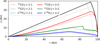 |
Fig. 1 Vertical τz = 1 emission surfaces for the two transitions (J = 2 − 1, J = 3 − 2) of each of the three isotopologues (12CO,13CO,C18O) in the initial condition for our fiducial protoplanetary disk. The black solid lines indicate simulation boundaries (in this case, rout = 100 au), while the dashed gray lines indicate wave-damping regions in the hydrodynamical simulations. The sharp transition in the 13COJ = 3 − 2 τz = 1 surface is caused by freeze-out of the immediately overlying material at large radii. |
3 Results
3.1 Spiral structure
We computed moment maps for our final simulations and for the initial condition using the bettermoments method (Teague & Foreman-Mackey 2018). A background model of this kind assumes a perfect knowledge of the disk properties, thus eliminating errors associated with prescribed semi-analytical τz = 1 surfaces, density, and velocity fields that would manifest in fits of real observations. Nevertheless, it retains the drawback that large-scale changes to the disk structure during the simulation would alter the τz = 1 surface. Thus, the differential moment maps we plotted include contributions from the change in velocity at each point in the disk over the simulation lifetime and from the shift in the emitting layer whose velocities are sampled. In Fig. 2 we plot the modeled line-of-sight velocity in each of our simulations, at various inclinations, in the J = 2 − 1 transition of the 12CO isotopologue. In Fig. 3 we show line-of-sight velocities in the J = 2 − 1 transitions of all three isotopologues (12CO, 13CO, C18O) at a fixed 0◦ inclination. In all cases, the moment-1 maps from the final simulations were regularized by subtracting the moment-1 computed from the initial condition. We present our full library of moment-1 maps in the Appendix (see Appendix B for a description, and the following sections for images).
We find that the three-temperature simulations manifest a clear two-armed shadow-driven kinematic spiral, strongest in the 12CO lines tracing the upper disk atmosphere and becoming progressively weaker in the deeper layers probed by 13CO and C18O, respectively. This is consistent with the fact that in our simulations the shadow is excited at the τr = 1 surface for stellar irradiation, and would thus not be expected to generate significant motion in the midplane (Muley et al. 2024a).
These shadow-driven spirals are strongest (v⊥ ≈ 200 m s−1) in the face-on case, but remain visible in 12COat a 30◦ inclination. At 60◦, they become all but invisible, particularly when beam convolution is considered. This geometrical effect evidences the strong vertical motions in the shadowed disk, driven by disk columns attempting to relax to hydrostatic equilibrium as the (sub-)Keplerian flow transports them into and out of shadowed regions (Muley et al. 2024a). Mathematically, this effect can be accounted for by including in-plane advection of vertical momentum – principally in the azimuthal direction – in the evaluation of hydrostatic equilibrium:
 (2)
(2)
This term was the subject of extensive discussion in Zhang & Zhu (2024), who demonstrated its importance in the context of shadow-driven spirals and discussed implications for kinematic observations.
The physical picture is very different for our multi-Jupiter-mass disk-planet interaction setup, in which we used β-cooling to an azimuthally symmetric background structure to preclude the development of shadow-driven spirals. In this case, there is no clear, open, two-armed kinematic spiral in any isotopologue, but rather a comparatively weak (v⊥ ≲ 1 100 m s− ) signal from the tightly wound, inner planetary spirals. These vertical-motion spirals are strongest in 12CO, and as shown in Muley et al. (2024b), can also be attributed to the effect of in-plane advection on hydrostatic equilibrium. However, given that the typical wavenumber of planet-driven Lindblad spirals (m ≈ (h/r)−1) is much larger than that of shadow-driven spirals in this case (m = 2), the former are significantly thinner and lose their distinctive morphology under beam convolution. Unlike in Bae et al. (2021), where a highly evolved well-settled grain size distribution leads to long cooling times – and consequently, robust buoyancy spirals – at the 12CO emission surface, the constant dust-to-gas ratio in our simulations means that collisional cooling is faster and buoyancy-related features are consequently weaker.
Such a high-mass planet opens a wide and deep gap, which is visible in the optically thinner 13CO and C18O isotopologues (see Appendices C and D) , whose emitting surfaces are closer to the midplane. In particular, the face-on 13CO images show vertical motions (∼50–100 m/s) at the inner gap edge, potentially attributable to the meridional flow patterns in Fung & Chiang (2016) or Bi et al. (2023). The polar accretion flow onto the planet (e.g., Fung et al. 2015; Schulik et al. 2019), of comparable magnitude, is also visible. At a 30-degree inclination these features become less prominent, but a prominent Doppler flip (e.g., Casassus & Pérez 2019; Pinte et al. 2022) associated with the in-plane motions generated by the planet comes into view (for further discussion, see Appendix B). All of these features are notably absent in our shadow-driven spiral model, given that the planet is of significantly lower mass in that case.
Our mock VLT/SPHERE H-band images, shown in Fig. 4, have high angular resolution, which makes them a useful complement to the kinematic maps. The planet-driven case builds on the work of Dong & Fung (2017), which sought to reproduce the substructures in the MWC 758 system using a model with similar properties to ours. In the present work, our use of a realistic vertically stratified temperature structure (Juhász & Rosotti 2018) causes wave refraction, and the non-isothermal equation of state reduces the density contrast across the spiral (e.g., Zhu et al. 2015; Muley et al. 2024b), contributing to a weakening of the planet-driven spiral, particularly in the disk atmosphere, which is the region probed by NIR observations. A simple visual fit using Archimedian spirals, overplotted on the mock images, shows that the shadow-driven spirals are both more open (pitch angle αs ≈ 0.24 vs. 0.14) and rotationally symmetric (angular separation ∆ϕs ≈ π/2 vs. 2π/3) than the planet-driven spirals.
Taken together, our results imply that a near-infrared double-armed spiral with a strong kinematic counterpart in the upper layer (12CO or 13CO), but weak when closer to the midplane (C18O), is likely shadow-driven, with the upper layers of the disk experiencing significant vertical expansion and contraction as their orbits take them through regions of greater or less illumination. By contrast, a near-infrared spiral with comparatively weaker kinematic spirals in the upper layer (such as 12CO or 13CO), is consistent with planetary driving, and thus a good candidate for direct-imaging searches. We grant, however, that depletion of CO would alter the height of each isotopologue’s emitting surface (Paneque-Carreño et al. 2025), and thus the disk layer whose properties it traces.
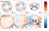 |
Fig. 2 Kinematic moment-1 (line-of-sight velocity) maps for the shadow-driven spirals, above, and the planet-driven spirals, below, in the J = 2 – 1 transition of the 12CO isotopologue; in each case, the moment-1 map of the initial condition is subtracted from that at the end of the simulation. From left to right, we plot disk inclinations of 0◦, 30◦, and 60◦. The FWHM of the fiducial ALMA beam (0.19′′ × 0.17′′) is indicated by a gray hatched ellipse. The spiral morphology is much more prominent in the shadow-driven case than in the spiral-driven case. |
3.2 Line broadening
In Fig. 5 we plot simulated line profiles in the optically thick J = 2 − 1 transition of the 12CO isotopologue, taken at a representative radial position R = 60 au and angular position ϕ = 0 with respect to the x-axis of Fig. 4. In the upper panel we plot the line from our shadow-driven spiral simulation, whereas in the lower panel we show the line from the planet-driven simulation, considering in both cases a face-on orientation. In the initial condition, these lines appear to be symmetric around v = 0 and only minimally affected by beam convolution; this is in⊥line with expectations because the average line-of-sight velocity is zero for an unperturbed face-on disk, and the only contribution to line width is thermal. Because ***(eq5)*** and ***(eq6)***
 and varies only weakly (∼10%) over the beam’s length scale at the fiducial Rline. Even this difference is significantly suppressed at first order by the approximate symmetry of the convolution kernel around Rline.
In an evolved disk, the presence of net upward and downward velocities at the emission surface moves the line center away from v⊥ = 0. This lowers the optical depths at the peak rest-frame wavelengths of the lines, allowing light from deeper layers (less perturbed by the spiral structure) to shine through, leading to a profile more complex than a simple, shifted initial condition. Both of these effects are more pronounced in the shadow-driven case than in the planet-driven case. Beam convolution, by averaging over regions of both positive and negative v⊥, contributes to additional line broadening (moment-2), while damping the measured v⊥ (or, equivalently, moment-1) to zero.
The moment-2 maps of the shadow- and planet-driven spirals in Fig. 6 both present a more qualitative view of the situation. In the planet-driven case, we observe a strong signal in the vicinity of the planet, corresponding to the hot polar accretion flows feeding the circumplanetary disk; the effects of this are visible to a lesser extent throughout the entire planetary corotation region. In the inner regions of the disk, where the planet-driven spirals become more tightly wound, we also find an elevated velocity dispersion. For the shadow-driven spiral, the morphology is altogether different, with the planetary gap surrounded by four separate regions of elevated velocity dispersion; these correspond to regions of strong shadowing where the kinematic spirals are launched. Beam convolution preserves this basic structure, although it smears out the specific details. A similar picture holds in the optically thinner 13CO and C18O iso-topologues (not shown here), although, as in the moment-1 case, the signals tend to be weaker. These differences in morphology provide yet another means of distinguishing planet-driven from shadow-driven sprial features.
Our analysis is similar to that of Dong et al. (2019), who likewise post-processed simulations of disk-planet interaction to study the line broadening caused by planet-induced flows. We built on their work by using a temperature structure self-consistently obtained using radiation hydrodynamics, rather than setting a constant unstratified background temperature. Moreover, we include the effects of beam convolution in order to facilitate comparison with actual observations. Although both works include a case of equivalent mass (Mp = 4 MJ), the disk aspect ratio is much smaller in their simulations (hp = 0.05) than in ours (hp ≈ 0.075), meaning their high-mass planet has a greater thermal mass. Consequently, the planet-carved gap is both deeper and narrower in their simulations (e.g., Dong et al. 2016), with fast and unsteady flows having established them throughout the gap. In radiative-transfer post-processing, this leads to significant line broadening throughout the gap, unlike in our work where such rapid flows, and consequently line broadening, are largely confined to the circumplanetary region.
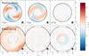 |
Fig. 3 Kinematic moment-1 (line-of-sight velocity) maps at the end of the simulation, with moment-1 from the initial condition subtracted, as in Fig. 2. In contrast to the plots in Fig. 2, we fix the disk inclination to 0◦ (face-on) and plot (from left to right) the maps corresponding to the J = 2 − 1 transitions of the 12CO , 13CO , and C18O isotopologues, which respectively trace the upper, intermediate, and midplane layers of the disk. In C18O, the two-armed signature of the shadow-driven spiral is virtually absent, but for the standard planet-driven case the inner Lindlbad spirals remain visible. |
3.3 Modal analysis
Fourier analysis can be used to provide an alternative view of shadow-driven spirals, emphasizing information that is difficult to discern from the images themselves. This exercise was carried out by Calcino et al. (2025) in order to characterize the spiral arms generated by infalling material in a protoplanetary disk. We adapted this technique for our purposes by using a Fourier transform on our mock observables (specifically, the moment-1 maps) rather than the simulated fluid quantities directly, and by considering more general disk inclinations than face-on. We deproject our mock observations using the following relation, assuming a zero position angle
 (3a)
(3a)
where
 (3b)
and ϕ represents the azimuthal angle with respect to the x-axis. As stated previously, we use disk inclinations id = {0◦, 30◦, 60◦} for our mock images. αiso is the angular elevation of the emitting layer of the transition in question, which we hold to be αiso = {0.24, 0.13, 0.07} for the J = 2 − 1 transitions of 12CO, 13CO, and C18O, respectively, and αiso = {0.275, 0.145, 0.085} for the J = 3 − 2 transitions of the same isotopologues.
(3b)
and ϕ represents the azimuthal angle with respect to the x-axis. As stated previously, we use disk inclinations id = {0◦, 30◦, 60◦} for our mock images. αiso is the angular elevation of the emitting layer of the transition in question, which we hold to be αiso = {0.24, 0.13, 0.07} for the J = 2 − 1 transitions of 12CO, 13CO, and C18O, respectively, and αiso = {0.275, 0.145, 0.085} for the J = 3 − 2 transitions of the same isotopologues.
In Fig. 7 we present a moment-1 power spectrum computed from the beam-convolved J = 2 − 1 12CO mock observations. As in the corresponding Fig. 2, the top row represents shadow-driven spirals and the bottom row planet-driven spirals, with the inclination increasing from left to right. In the face-on case, the power is concentrated in the m = 2 modes (and more generally in even-numbered modes) in the shadow-driven case; in the standard planet-driven case, the power shows no such bias toward even wavenumbers. We caution, however, that this result holds only for low mass ratios between the primary and companion; for higher ratios, particularly when the system is an equal binary, the m = 2 mode can come to dominate the potential and thus, the shape of the companion-driven spirals (Artymowicz & Lubow 1994).
As the disk inclination increases, this distinction fades, as the difference in sky-projected area between the near and far sides of the disk, as well as the contribution of the vr and vϕ to the line-of-sight velocity, introduces odd frequency content even in the shadow-driven case. The vϕ component in particular, which represents fast quasi-Keplerian background flow, introduces artifacts in the moment-1 maps whenever it varies on a length scale shorter than the beam-convolution scale. These artifacts are most prominent in the inner disk (and grow with increasing inclination due to sky-projection effects) and in Fourier space, and manifest as high-frequency content. Computing the true first moment of the spectrum – as opposed to using bettermoments, which estimates the line centroid – would mitigate these issues, but at the cost of suppressing features in the outer disk.
In Fig. 8 we present the power spectra for the J = 2 − 1 transitions of all three of the CO isotopologues in our work, following the pattern of Fig. 3; the presented disks are all face-on. As in Fig. 7, we see that even-numbered modes in general, and the m = 2 mode in particular, are strong for the shadow-driven case. The power in m = 2 is weaker for 13CO than for 12CO, and for C18O weaker still. As previously mentioned, the planet-driven case differs from the shadow-driven case in that its power spectrum contains odd frequency content; moreover, we find that there is no clear trend in mode strength with respect to the altitude of the optical surface of the relevant transition. We attribute the higher-order harmonics in the power spectra of 13CO in the shadow-driven case, and C18O in the spiral-driven case, to the sharp interfaces created by bettermoments between the approaching and receding regions.
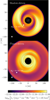 |
Fig. 4 Modeled NIR image in the H-band (λH = 1.62 µm of the shadow-driven (above) and planet-driven (below) spiral cases. In each panel, the location of the planet is identified with a white dot, and an Archimedian spiral fit is shown as gray dashed lines. The beam is indicated with a gray hatched ellipse, while the effect of a coronagraph is mimicked by the black circle 20 au (0.2′′) in radius. The standard planetary Lindblad spirals are weakened in the disk atmosphere (traced by NIR scattering off the entrained dust grains) by wave refraction at the temperature transition corresponding to the disk’s τr = 1 surface. |
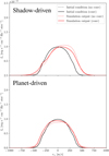 |
Fig. 5 12COJ = 2 − 1 lines, for the planet-driven spiral models (above) and the shadow-driven models (below), at a position R = 60 au and ϕ = 0 with respect to the x-axes of Fig. 4 (and, equivalently, of the qualitative maps in Fig. 6). In the initial condition, line broadening results exclusively from thermal motion, and is largely unaffected by beam convolution. In evolved disks, however, the line profile is shifted and broadened by vertical motions within spiral arms, with beam convolution over regions of differing velocity dampening the overall directional shift, while enhancing broadening. |
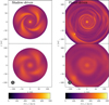 |
Fig. 6 Maps of the typical line-of-sight velocity dispersion along each line of sight in the J = 2 − 1 transition of 12CO, for the shadow-driven case (left) and the planet-driven case (right). The upper panels are computed from the raw datacubes, while the lower panels are computed from the datacubes convolved with the fiducial beam. In the planet-driven case, we see a strong localized increase in velocity dispersion near the planet location, and in the interior of the disk; in the shadow-driven case we see four separate peaks along the outer edge of the gap, corresponding to the launching points of the spirals. |
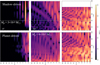 |
Fig. 7 Fourier transforms of moment-1 maps constructed from beam-convolved 12CO J = 2 − 1 datacubes. As in Fig. 2, we plot the shadow-driven case in the upper row, and the more standard planet-driven case in the lower, with inclinations of 0◦, 30◦, and 60◦ (from left to right). We indicate the planet’s radial location in each case with a dotted line. For the shadow-driven spiral, the power is most concentrated in even-numbered modes, a feature absent from the classical case; however, this distinction becomes less apparent in the inclined cases. To avoid contamination of the mode structure due to emission from the (unphysically situated) outer radial boundary of the simulation, we clip large radii from our plot for the id = 30◦ and 60◦ cases. |
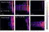 |
Fig. 8 Modal plots for moment-1 maps constructed from beam-convolved datacubes. From left to right, we show modal plots associated with the J = 2 − 1 transitions of 12CO, 13CO, and C18O, respectively, fixing the inclination to 0◦. We indicate the planet’s radial location in each case with a dotted line. As in Fig. 7, the shadow-driven case is above, while the planet-driven case is below. Shadow-driven spirals show an m = 2 mode steadily decreasing in strength with deeper and deeper isotopologues. |
4 Conclusions
With the PLUTO hydrodynamics code, we re-ran one of the radiative-hydrodynamics simulations in Muley et al. (2024a), in which two-armed shadow-driven spirals were seen to develop exterior to sufficiently deep planet-carved gaps in protoplan-etary disks. For comparison, we also ran a simulation with β-cooling and a widely separated multi-Jupiter-mass planet, which drove two-armed interior spirals according to the classical theory of disk-planet interaction (Goldreich & Tremaine 1978, 1979; Bae & Zhu 2018a). Using the RADMC3D MCRT code, we post-processed these simulations to obtain mock images and datacubes in wavelengths tracing both gas and small entrained dust grains. These were analyzed to produce moment maps, line profiles, and modal decompositions, which encode telltale signs of the underlying spiral driving mechanism.
Specifically, we find that the double-armed shadow-driven spirals in Muley et al. (2024a) are associated with strong kinematic signatures, particularly when viewed face-on, due to the substantial vertical motion associated with shadow-driven spirals. By contrast, the double-armed inner Lindblad spirals produced in the classical picture of disk-planet interaction are of comparatively limited prominence in the kinematics. Beyond intrinsic differences in the sky-projected velocity profiles, the higher wavenumbers of the planet-driven spirals with respect to the shadow-driven ones (m ≈ 1/h versus m = 2) mean their angular widths are smaller, meaning that they can be more easily washed out by beam convolution. In Fourier space, the moment-1 maps of spirals driven by shadows and by planetary-mass companions can be distinguished in face-on observations by the predominantly even frequency content of the former. For inclined disks, the differing angles of the optical surfaces on either side of the disk with respect to the plane of the sky create a bilateral asymmetry in the projected sizes of disk features, introducing odd frequency content even in the shadow-driven case.
The kinematic signatures we identify would be accessible to surveys such as exoALMA (Teague et al. 2025, and subsequent papers in series), and would provide a useful heuristic to distinguish between potentially shadow-driven and classically planet-driven cases in systems with two-armed spiral structure in scattered light. The exterior, multi-Jupiter-mass planets required to trigger the latter mechanism would, in turn, be particularly promising targets for direct-imaging campaigns1.
We envision our study as a starting point for a wide range of potential future investigations. In addition to shadows and classical disk-planet interaction, other mechanisms (e.g., infalling gas Kuznetsova et al. 2022; Hühn et al. 2025, stellar flybys Smallwood et al. 2023, and gravitational instability Dong et al. 2015a) are also capable of creating m = 2 spirals, and it would be worthwhile to use simulations and MCRT post-processing to study their distinguishing features in molecular lines and near-infrared scattered light. Within the existing scope, short characteristics (Davis et al. 2012), discrete ordinates (Jiang 2021), or half-moment methods (Melon Fuksman et al. 2025) are capable of accommodating crossing light beams, making the disk’s temperature structure more accurate, improving the handling of shadows, and enabling the incorporation of accreting planets alongside shadow-driven spirals. Additionally, one could vary the dust-to-gas ratio or grain size distribution, and with it, the gas-grain thermal coupling time. Not only might this affect the shadow-driving mechanism – dependent as it is on the response of the disk to radiation – but also disk-planet interaction itself. For long thermal relaxation times, planets are known to excite spirals at buoyancy resonances (Zhu et al. 2012; Lubow & Zhu 2014), typified by strong vertical motions near the planet’s orbital radius. Such spirals, distinct in morphology from shadow-driven vertical motions, would produce their own kinematic signatures (Bae et al. 2021) and serve as signposts of the planet’s existence.
In post-processing, testing different isotopologue ratios and concentrations would change the emitting layers, providing better coverage of the full parameter space spanned by observed systems. More ambitiously, one could use a radiative-transfer code capable of computing non-LTE level populations from the radiation field, such as SPARX2 or SKIRT (Matsumoto et al. 2023). One could also move beyond convolving mock images with a Gaussian beam, and make use of the ALMA-specific CASA pipeline to construct more realistic mock observations. This would be of particular value in the context of our modal analysis; our current approach necessarily restricts us to a Fourier transform for the image-plane moment-1 maps, but it may be worthwhile to see if the telltale spectral patterns of shadow- and planet-driven spirals are visible in the uv-plane. In addition, the use of such tools would offer insights into the telescope configurations and on-source time required to identify features of interest (e.g., Speedie et al. 2022).
The present study underscores the importance of using disk observations at different wavelengths, thus tracing different layers and components, when trying to constrain the underlying physical scenario giving rise to its morphology. A natural extension would also be to model the millimeter and submillimeter emission, which traces the large-dust population, and has been of significant interest to observational campaigns (e.g., DSHARP Andrews et al. 2018) aimed at understanding disk substructure. The simplest approach would be to take a hydrodynamical snapshot, and use equilibrium prescriptions for the vertical settling and radial accumulation of large grains to compute their density field for radiative-transfer post-processing (e.g., Hashimoto et al. 2015; Dullemond et al. 2018; Muley et al. 2019; Brown-Sevilla et al. 2021). However, the fact that disk-planet interaction is a dynamical problem makes it highly desirable to self-consistently incorporate the kinematic and thermal coupling between gas, dust, and radiation during the hydrodynamical simulations themselves. While schemes for multispecies dust dynamics exist (e.g., Benítez-Llambay et al. 2019; Huang & Bai 2022; Krapp et al. 2024), multispecies thermodynamics would require generalizing the existing three-temperature scheme of Muley et al. (2023). This is a substantial undertaking requiring the development and testing of new numerical methods, which we defer to future studies.
Acknowledgements
We thank Jiaqing Bi, Til Birnstiel, Mario Flock, Margot Leemker, Anna Penzlin, Matthias Samland, Volker Springel, and Alexandros Ziampras for useful discussions which improved the quality of this work. Furthermore, we thank the referee for a helpful and informative report. Numerical simulations were carried out on the Raven cluster of the Max-Planck-Gesellschaft and the Vera Cluster of the Max-Planck-Institut für Astronomie, both hosted by the Max Planck Computing and Data Facility (MPCDF) in Garching bei München.
References
- Andrews, S. M., Huang, J., Pérez, L. M., et al. 2018, ApJ, 869, L41 [NASA ADS] [CrossRef] [Google Scholar]
- Artymowicz, P., & Lubow, S. H. 1994, ApJ, 421, 651 [Google Scholar]
- Asensio-Torres, R., Henning, T., Cantalloube, F., et al. 2021, A&A, 652, A101 [NASA ADS] [CrossRef] [EDP Sciences] [Google Scholar]
- Bae, J., & Zhu, Z. 2018a, ApJ, 859, 118 [Google Scholar]
- Bae, J., & Zhu, Z. 2018b, ApJ, 859, 119 [Google Scholar]
- Bae, J., Teague, R., & Zhu, Z. 2021, ApJ, 912, 56 [NASA ADS] [CrossRef] [Google Scholar]
- Barraza-Alfaro, M., Flock, M., Marino, S., & Pérez, S. 2021, A&A, 653, A113 [NASA ADS] [CrossRef] [EDP Sciences] [Google Scholar]
- Barraza-Alfaro, M., Flock, M., & Henning, T. 2024, A&A, 683, A16 [NASA ADS] [CrossRef] [EDP Sciences] [Google Scholar]
- Benítez-Llambay, P., Krapp, L., & Pessah, M. E. 2019, ApJS, 241, 25 [Google Scholar]
- Béthune, W., Latter, H., & Kley, W. 2021, A&A, 650, A49 [NASA ADS] [CrossRef] [EDP Sciences] [Google Scholar]
- Bi, J., Lin, M.-K., & Dong, R. 2023, ApJ, 942, 80 [NASA ADS] [CrossRef] [Google Scholar]
- Biddle, L. I., Bowler, B. P., Zhou, Y., Franson, K., & Zhang, Z. 2024, arXiv e-prints [arXiv:2402.12601] [Google Scholar]
- Brown-Sevilla, S. B., Keppler, M., Barraza-Alfaro, M., et al. 2021, A&A, 654, A35 [NASA ADS] [CrossRef] [EDP Sciences] [Google Scholar]
- Calcino, J., Price, D. J., Hilder, T., et al. 2025, MNRAS, 537, 2695 [Google Scholar]
- Casassus, S., & Pérez, S. 2019, ApJ, 883, L41 [Google Scholar]
- Cugno, G., Leisenring, J., Wagner, K. R., et al. 2024, AJ, 167, 182 [NASA ADS] [CrossRef] [Google Scholar]
- Cugno, G., Facchini, S., Alarcon, F., et al. 2025, arXiv e-prints [arXiv:2509.26617] [Google Scholar]
- Davis, S. W., Stone, J. M., & Jiang, Y.-F. 2012, ApJS, 199, 9 [NASA ADS] [CrossRef] [Google Scholar]
- Desidera, S., Chauvin, G., Bonavita, M., et al. 2021, A&A, 651, A70 [EDP Sciences] [Google Scholar]
- Dong, R., & Fung, J. 2017, ApJ, 835, 38 [Google Scholar]
- Dong, R., Hall, C., Rice, K., & Chiang, E. 2015a, ApJ, 812, L32 [Google Scholar]
- Dong, R., Zhu, Z., Rafikov, R. R., & Stone, J. M. 2015b, ApJ, 809, L5 [Google Scholar]
- Dong, R., Fung, J., & Chiang, E. 2016, ApJ, 826, 75 [Google Scholar]
- Dong, R., Liu, S.-Y., & Fung, J. 2019, ApJ, 870, 72 [NASA ADS] [CrossRef] [Google Scholar]
- Dullemond, C. P., Birnstiel, T., Huang, J., et al. 2018, ApJ, 869, L46 [NASA ADS] [CrossRef] [Google Scholar]
- Ercolano, B., & Picogna, G. 2022, Euro. Phys. J. Plus, 137, 1357 [Google Scholar]
- Flock, M., Ruge, J. P., Dzyurkevich, N., et al. 2015, A&A, 574, A68 [NASA ADS] [CrossRef] [EDP Sciences] [Google Scholar]
- Follette, K. B., Close, L. M., Males, J. R., et al. 2023, AJ, 165, 225 [NASA ADS] [CrossRef] [Google Scholar]
- Fung, J., & Chiang, E. 2016, ApJ, 832, 105 [NASA ADS] [CrossRef] [Google Scholar]
- Fung, J., & Dong, R. 2015, ApJ, 815, L21 [NASA ADS] [CrossRef] [Google Scholar]
- Fung, J., Shi, J.-M., & Chiang, E. 2014, ApJ, 782, 88 [NASA ADS] [CrossRef] [Google Scholar]
- Fung, J., Artymowicz, P., & Wu, Y. 2015, ApJ, 811, 101 [Google Scholar]
- Goldreich, P., & Tremaine, S. 1978, ApJ, 222, 850 [NASA ADS] [CrossRef] [Google Scholar]
- Goldreich, P., & Tremaine, S. 1979, ApJ, 233, 857 [Google Scholar]
- Goldreich, P., & Tremaine, S. 1980, ApJ, 241, 425 [Google Scholar]
- Grady, C. A., Muto, T., Hashimoto, J., et al. 2013, ApJ, 762, 48 [Google Scholar]
- Hashimoto, J., Tsukagoshi, T., Brown, J. M., et al. 2015, ApJ, 799, 43 [CrossRef] [Google Scholar]
- Hu, X., Li, Z.-Y., Zhu, Z., & Yang, C.-C. 2022, MNRAS, 516, 2006 [NASA ADS] [CrossRef] [Google Scholar]
- Huang, P., & Bai, X.-N. 2022, ApJS, 262, 11 [NASA ADS] [CrossRef] [Google Scholar]
- Hühn, L. A., Jiang, H. C., & Dullemond, C. P. 2025, A&A, 701, L15 [NASA ADS] [CrossRef] [EDP Sciences] [Google Scholar]
- Isella, A., Guidi, G., Testi, L., et al. 2016, Phys. Rev. Lett., 117, 251101 [NASA ADS] [CrossRef] [Google Scholar]
- Jiang, Y.-F. 2021, ApJS, 253, 49 [NASA ADS] [CrossRef] [Google Scholar]
- Juhász, A., & Rosotti, G. P. 2018, MNRAS, 474, L32 [Google Scholar]
- Krapp, L., Garrido-Deutelmoser, J., Benítez-Llambay, P., & Kratter, K. M. 2024, ApJS, 271, 7 [NASA ADS] [CrossRef] [Google Scholar]
- Krieger, A., & Wolf, S. 2020, A&A, 635, A148 [NASA ADS] [CrossRef] [EDP Sciences] [Google Scholar]
- Kuznetsova, A., Bae, J., Hartmann, L., & Mac Low, M.-M. 2022, ApJ, 928, 92 [NASA ADS] [CrossRef] [Google Scholar]
- Lubow, S. H., & Zhu, Z. 2014, ApJ, 785, 32 [NASA ADS] [CrossRef] [Google Scholar]
- Maio, F., Fedele, D., Roccatagliata, V., et al. 2025, A&A, 699, L10 [NASA ADS] [CrossRef] [EDP Sciences] [Google Scholar]
- Matsumoto, K., Camps, P., Baes, M., et al. 2023, A&A, 678, A175 [NASA ADS] [CrossRef] [EDP Sciences] [Google Scholar]
- Melon Fuksman, J. D., & Klahr, H. 2022, ApJ, 936, 16 [NASA ADS] [CrossRef] [Google Scholar]
- Melon Fuksman, J. D., & Mignone, A. 2019, ApJS, 242, 20 [NASA ADS] [CrossRef] [Google Scholar]
- Melon Fuksman, J. D., Klahr, H., Flock, M., & Mignone, A. 2021, ApJ, 906, 78 [NASA ADS] [CrossRef] [Google Scholar]
- Melon Fuksman, D., Flock, M., Klahr, H., Mattia, G., & Muley, D. 2025, A&A, 701, A97 [NASA ADS] [CrossRef] [EDP Sciences] [Google Scholar]
- Mignone, A., Bodo, G., Massaglia, S., et al. 2007, ApJS, 170, 228 [Google Scholar]
- Montesinos, M., & Cuello, N. 2018, MNRAS, 475, L35 [NASA ADS] [CrossRef] [Google Scholar]
- Montesinos, M., Perez, S., Casassus, S., et al. 2016, ApJ, 823, L8 [Google Scholar]
- Muley, D., Fung, J., & van der Marel, N. 2019, ApJ, 879, L2 [NASA ADS] [CrossRef] [Google Scholar]
- Muley, D., Melon Fuksman, J. D., & Klahr, H. 2023, A&A, 678, A162 [NASA ADS] [CrossRef] [EDP Sciences] [Google Scholar]
- Muley, D., Melon Fuksman, J. D., & Klahr, H. 2024a, A&A, 690, A355 [NASA ADS] [CrossRef] [EDP Sciences] [Google Scholar]
- Muley, D., Melon Fuksman, J. D., & Klahr, H. 2024b, A&A, 687, A213 [NASA ADS] [CrossRef] [EDP Sciences] [Google Scholar]
- Muto, T., Grady, C. A., Hashimoto, J., et al. 2012, ApJ, 748, L22 [Google Scholar]
- Paneque-Carreño, T., Miotello, A., van Dishoeck, E. F., Rosotti, G., & Tabone, B. 2025, A&A, 698, A231 [NASA ADS] [CrossRef] [EDP Sciences] [Google Scholar]
- Pinte, C., Ménard, F., Duchêne, G., et al. 2018a, A&A, 609, A47 [NASA ADS] [CrossRef] [EDP Sciences] [Google Scholar]
- Pinte, C., Price, D. J., Ménard, F., et al. 2018b, ApJ, 860, L13 [Google Scholar]
- Pinte, C., van der Plas, G., Ménard, F., et al. 2019, Nat. Astron., 3, 1109 [NASA ADS] [CrossRef] [Google Scholar]
- Pinte, C., Teague, R., Flaherty, K., et al. 2022, arXiv e-prints [arXiv:2203.09528] [Google Scholar]
- Ren, B., Dong, R., Esposito, T. M., et al. 2018, ApJ, 857, L9 [Google Scholar]
- Ren, B., Dong, R., van Holstein, R. G., et al. 2020, ApJ, 898, L38 [NASA ADS] [CrossRef] [Google Scholar]
- Ren, B. B., Xie, C., Benisty, M., et al. 2024, A&A, 681, L2 [NASA ADS] [CrossRef] [EDP Sciences] [Google Scholar]
- Schulik, M., Johansen, A., Bitsch, B., & Lega, E. 2019, A&A, 632, A118 [NASA ADS] [CrossRef] [EDP Sciences] [Google Scholar]
- Shuai, L., Ren, B. B., Dong, R., et al. 2022, ApJS, 263, 31 [NASA ADS] [CrossRef] [Google Scholar]
- Smallwood, J. L., Yang, C.-C., Zhu, Z., et al. 2023, MNRAS, 521, 3500 [NASA ADS] [CrossRef] [Google Scholar]
- Speedie, J., Booth, R. A., & Dong, R. 2022, ApJ, 930, 40 [NASA ADS] [CrossRef] [Google Scholar]
- Su, Z., & Bai, X.-N. 2024, ApJ, 975, 126 [Google Scholar]
- Teague, R., & Foreman-Mackey, D. 2018, Res. Notes AAS, 2, 173 [Google Scholar]
- Teague, R., Bae, J., Huang, J., & Bergin, E. A. 2019, ApJ, 884, L56 [Google Scholar]
- Teague, R., Bae, J., Aikawa, Y., et al. 2021a, ApJS, 257, 18 [NASA ADS] [CrossRef] [Google Scholar]
- Teague, R., Law, C. J., Huang, J., & Meng, F. 2021b, J. Open Source Softw., 6, 3827 [NASA ADS] [CrossRef] [Google Scholar]
- Teague, R., Bae, J., Andrews, S. M., et al. 2022, ApJ, 936, 163 [NASA ADS] [CrossRef] [Google Scholar]
- Teague, R., Benisty, M., Facchini, S., et al. 2025, ApJ, 984, L6 [Google Scholar]
- Wagner, K., Stone, J. M., Spalding, E., et al. 2019, ApJ, 882, 20 [Google Scholar]
- Wagner, K., Stone, J., Skemer, A., et al. 2023, Nat. Astron., 7, 1208 [CrossRef] [Google Scholar]
- Wagner, K., Leisenring, J., Cugno, G., et al. 2024, AJ, 167, 181 [NASA ADS] [CrossRef] [Google Scholar]
- Xie, C., Xie, C., Ren, B. B., et al. 2024, Universe, 10, 465 [Google Scholar]
- Zhang, M., Huang, P., & Dong, R. 2024, ApJ, 961, 86 [NASA ADS] [CrossRef] [Google Scholar]
- Zhang, S., & Zhu, Z. 2024, ApJ, 974, L38 [Google Scholar]
- Zhu, Z., Stone, J. M., & Rafikov, R. R. 2012, ApJ, 758, L42 [NASA ADS] [CrossRef] [Google Scholar]
- Zhu, Z., Dong, R., Stone, J. M., & Rafikov, R. R. 2015, ApJ, 813, 88 [Google Scholar]
- Zhu, Z., Zhang, S., & Johnson, T. M. 2025, ApJ, 980, 259 [Google Scholar]
- Ziampras, A., Dullemond, C. P., Birnstiel, T., Benisty, M., & Nelson, R. P. 2025, MNRAS, 540, 1185 [Google Scholar]
Interior planets associated with shadow-driven, gap-edge spirals would be less detectable due to lower contrast, and because their masses need not be super-Jupiter. In exceptionally high-mass cases, however (for instance, the putative detection in SAO 206462 by Maio et al. 2025), they may nevertheless be detectable.
Appendix A Total versus differential moment-1 maps
The figures presented in the main text show differential/residual moment maps, in which the line-of-sight velocities from the final simulations (computed using bettermoments) are regularized by subtracting off the line-of-sight velocities obtained from a background disk model. In this work, we choose for our background model a moment-1 map computed with RADMC3D from the simulation’s initial condition, which naturally reproduces the location of the optical surface for each transition, as well as the background velocities (giving the line shift) and temperatures (giving the width) on this surface. In Fig. A.1 we plot both the final and initial (background) moment-1 maps, computed from both raw and beam-convolved mock J = 2 − 1 12CO observations. In the face-on case, the background line-of-sight velocity is zero because the disk is in vertical hydrostatic equilibrium, but in inclined disks it becomes substantial, as the projection of the disk’s quasi-Keplerian velocity onto the line-of-sight becomes nonzero. In the inner regions of inclined disks, where approaching and receding quasi-Keplerian flows occur in close angular proximity to one another, beam convolution averages these together to yield no net apparent line-of-sight velocity.
Although our choice of an initial condition-based background model is logical and advantageous in many respects, limitations exist on its applicability to actual observations. Unlike in simulations, there is no way to determine a priori the unperturbed state of a real disk, while holding all other factors constant. Obtaining a physically informed, best-fit initial model would not only be highly expensive—due to the need to iterate MCRT and hydrostatic calculations (Melon Fuksman & Klahr 2022) at each sampled point in a multidimensional parameter space—but also degenerate in parameters such as disk mass, grain size distribution, opacity/mineralogy, and isotopologue mass fraction, among others. In practice, the emission surfaces of observed disks are often computed directly from channel maps (Pinte et al. 2018a; Teague et al. 2021b), with background velocities and temperatures found by fits to the azimuthally averaged measurements rather than detailed physical modeling.
Appendix B Full library of differential moment-1 maps
In what follows, we present mock bettermoments moment-1 maps of the disk with the shadow-driven spiral, for all of the transitions and isotopologues under consideration for our study. These are, namely, the J = 2 − 1 and 3 − 2 for 12CO, 13CO, and C18 transitions O. As in the main text, we regularize by subtracting off the moment-1 map produced from the initial condition, in order to reveal the spiral structure.
In these Appendix plots, however, we include moment maps computed both from the beam-convolved images, as well as those from non-convolved images. The latter reveal additional structure, especially in the inner disk and at higher inclination, which could potentially be probed by future, higher-resolution gas observations. However, they also show much stronger impact from artifacts generated by the bettermoments method itself, which the dissipative effect of beam convolution acts to mitigate.
In general, features are very similar in the J = 2 − 1 and J = 3−2 transitions of any given isotopologue, an unsurprising result given that both trace similar regions of the disk (Fig. 1). Shadow-driven features in 13CO and C18O are not as strong as those in 12CO—as demonstrated for face-on disks in the main text—and become weaker still when the system is viewed at an inclination id = 30◦, particularly when beam convolution is applied.
For the planet-driven case, we see that id = 30◦ shows the spiral structure much more clearly than does a face-on orientation (id = 0◦). This follows from the fact that in-plane velocity perturbations (vr, vϕ) dominate over vθ in classical disk-planet interaction, and that a nonzero inclination projects the in-plane components onto the line of sight. Indeed, in 13CO (Fig. D.2) and to a lesser extent C18O (Fig. D.3), the images at id = 30◦ empha-size the double-armed nature of the spiral. These images also clearly illustrate the Doppler-flip phenomenon associated with the planet’s location, which remains prominent even when beam convolution is considered.
In nearly all cases, save for the 12CO maps for the shadow-driven case, and the unconvolved 12CO maps for the planet-driven case, an inclination id = 60◦ makes it difficult to obtain useful information about the spirals therein from the observed gas kinematics. Nevertheless, alternative features, such as gaps and rings in ALMA dust continuum, may provide evidence for planet formation even in relatively high-inclination disks (Isella et al. 2016).
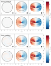 |
Fig. A.1 Kinematic moment-1 maps for the J = 2 − 1 transition of 12CO in the shadow-driven spiral simulations. Here the initial and final maps are plotted separately, unlike in the other figures where the former is used as a background model and subtracted from the latter. Accordingly, the range of the color scale (−5 km s−1 ≤ v⊥ ≤ 5 km s−1 ) was expanded to accommodate the Keplerian flow of the disk. |
Appendix C Shadow-driven spirals
Appendix C.1 12CO
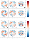 |
Fig. C.1 Kinematic moment-1 (line-of-sight velocity) maps of shadow-driven spirals in 12CO. The upper two rows are the J = 2 − 1 transition, while the lower two are for J = 3 − 2. From left to right, we plot disk inclinations of 0◦, 30◦, and 60◦. |
Appendix C.2 13CO
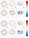 |
Fig. C.2 Kinematic moment-1 (line-of-sight velocity) maps of shadow-driven spirals in 13CO. The upper two rows are the J = 2 − 1 transition, while the lower two are for J = 3 − 2. From left to right, we plot disk inclinations of 0◦, 30◦, and 60◦. |
Appendix C.3 C18O
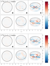 |
Fig. C.3 Kinematic moment-1 (line-of-sight velocity) maps of shadow-driven spirals in C18O. The upper two rows are the J = 2 − 1 transition, while the lower two are for J = 3 − 2. From left to right, we plot disk inclinations of 0◦, 30◦, and 60◦. |
Appendix D Planet-driven spirals
Appendix D.1 12CO
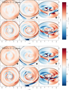 |
Fig. D.1 Kinematic moment-1 (line-of-sight velocity) maps of planet-driven spirals in 12CO. The upper two rows are the J = 2 − 1 transition, while the lower two are J = 3 − 2. From left to right, we plot disk inclinations of 0◦, 30◦, and 60◦. |
Appendix D.2 13CO
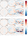 |
Fig. D.2 Kinematic maps of planet-driven spirals in 13CO. From left to right, we plot disk inclinations of 0◦, 30◦, and 60◦. The images at 30◦ in particular reveal the planet-driven spiral structure, as well as the Doppler flip at the planet’s location. |
Appendix D.3 C18O
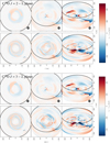 |
Fig. D.3 Kinematic maps of planet-driven spirals in C18O. From left to right, we plot disk inclinations of 0◦, 30◦, and 60◦. The Doppler flip remains prominent in the moderate-inclination case, although the spiral signature itself is degraded by bettermoments artifacts. |
All Figures
|
Fig. 1 Vertical τz = 1 emission surfaces for the two transitions (J = 2 − 1, J = 3 − 2) of each of the three isotopologues (12CO,13CO,C18O) in the initial condition for our fiducial protoplanetary disk. The black solid lines indicate simulation boundaries (in this case, rout = 100 au), while the dashed gray lines indicate wave-damping regions in the hydrodynamical simulations. The sharp transition in the 13COJ = 3 − 2 τz = 1 surface is caused by freeze-out of the immediately overlying material at large radii. |
| In the text | |
|
Fig. 2 Kinematic moment-1 (line-of-sight velocity) maps for the shadow-driven spirals, above, and the planet-driven spirals, below, in the J = 2 – 1 transition of the 12CO isotopologue; in each case, the moment-1 map of the initial condition is subtracted from that at the end of the simulation. From left to right, we plot disk inclinations of 0◦, 30◦, and 60◦. The FWHM of the fiducial ALMA beam (0.19′′ × 0.17′′) is indicated by a gray hatched ellipse. The spiral morphology is much more prominent in the shadow-driven case than in the spiral-driven case. |
| In the text | |
|
Fig. 3 Kinematic moment-1 (line-of-sight velocity) maps at the end of the simulation, with moment-1 from the initial condition subtracted, as in Fig. 2. In contrast to the plots in Fig. 2, we fix the disk inclination to 0◦ (face-on) and plot (from left to right) the maps corresponding to the J = 2 − 1 transitions of the 12CO , 13CO , and C18O isotopologues, which respectively trace the upper, intermediate, and midplane layers of the disk. In C18O, the two-armed signature of the shadow-driven spiral is virtually absent, but for the standard planet-driven case the inner Lindlbad spirals remain visible. |
| In the text | |
|
Fig. 4 Modeled NIR image in the H-band (λH = 1.62 µm of the shadow-driven (above) and planet-driven (below) spiral cases. In each panel, the location of the planet is identified with a white dot, and an Archimedian spiral fit is shown as gray dashed lines. The beam is indicated with a gray hatched ellipse, while the effect of a coronagraph is mimicked by the black circle 20 au (0.2′′) in radius. The standard planetary Lindblad spirals are weakened in the disk atmosphere (traced by NIR scattering off the entrained dust grains) by wave refraction at the temperature transition corresponding to the disk’s τr = 1 surface. |
| In the text | |
|
Fig. 5 12COJ = 2 − 1 lines, for the planet-driven spiral models (above) and the shadow-driven models (below), at a position R = 60 au and ϕ = 0 with respect to the x-axes of Fig. 4 (and, equivalently, of the qualitative maps in Fig. 6). In the initial condition, line broadening results exclusively from thermal motion, and is largely unaffected by beam convolution. In evolved disks, however, the line profile is shifted and broadened by vertical motions within spiral arms, with beam convolution over regions of differing velocity dampening the overall directional shift, while enhancing broadening. |
| In the text | |
|
Fig. 6 Maps of the typical line-of-sight velocity dispersion along each line of sight in the J = 2 − 1 transition of 12CO, for the shadow-driven case (left) and the planet-driven case (right). The upper panels are computed from the raw datacubes, while the lower panels are computed from the datacubes convolved with the fiducial beam. In the planet-driven case, we see a strong localized increase in velocity dispersion near the planet location, and in the interior of the disk; in the shadow-driven case we see four separate peaks along the outer edge of the gap, corresponding to the launching points of the spirals. |
| In the text | |
|
Fig. 7 Fourier transforms of moment-1 maps constructed from beam-convolved 12CO J = 2 − 1 datacubes. As in Fig. 2, we plot the shadow-driven case in the upper row, and the more standard planet-driven case in the lower, with inclinations of 0◦, 30◦, and 60◦ (from left to right). We indicate the planet’s radial location in each case with a dotted line. For the shadow-driven spiral, the power is most concentrated in even-numbered modes, a feature absent from the classical case; however, this distinction becomes less apparent in the inclined cases. To avoid contamination of the mode structure due to emission from the (unphysically situated) outer radial boundary of the simulation, we clip large radii from our plot for the id = 30◦ and 60◦ cases. |
| In the text | |
|
Fig. 8 Modal plots for moment-1 maps constructed from beam-convolved datacubes. From left to right, we show modal plots associated with the J = 2 − 1 transitions of 12CO, 13CO, and C18O, respectively, fixing the inclination to 0◦. We indicate the planet’s radial location in each case with a dotted line. As in Fig. 7, the shadow-driven case is above, while the planet-driven case is below. Shadow-driven spirals show an m = 2 mode steadily decreasing in strength with deeper and deeper isotopologues. |
| In the text | |
|
Fig. A.1 Kinematic moment-1 maps for the J = 2 − 1 transition of 12CO in the shadow-driven spiral simulations. Here the initial and final maps are plotted separately, unlike in the other figures where the former is used as a background model and subtracted from the latter. Accordingly, the range of the color scale (−5 km s−1 ≤ v⊥ ≤ 5 km s−1 ) was expanded to accommodate the Keplerian flow of the disk. |
| In the text | |
|
Fig. C.1 Kinematic moment-1 (line-of-sight velocity) maps of shadow-driven spirals in 12CO. The upper two rows are the J = 2 − 1 transition, while the lower two are for J = 3 − 2. From left to right, we plot disk inclinations of 0◦, 30◦, and 60◦. |
| In the text | |
|
Fig. C.2 Kinematic moment-1 (line-of-sight velocity) maps of shadow-driven spirals in 13CO. The upper two rows are the J = 2 − 1 transition, while the lower two are for J = 3 − 2. From left to right, we plot disk inclinations of 0◦, 30◦, and 60◦. |
| In the text | |
|
Fig. C.3 Kinematic moment-1 (line-of-sight velocity) maps of shadow-driven spirals in C18O. The upper two rows are the J = 2 − 1 transition, while the lower two are for J = 3 − 2. From left to right, we plot disk inclinations of 0◦, 30◦, and 60◦. |
| In the text | |
|
Fig. D.1 Kinematic moment-1 (line-of-sight velocity) maps of planet-driven spirals in 12CO. The upper two rows are the J = 2 − 1 transition, while the lower two are J = 3 − 2. From left to right, we plot disk inclinations of 0◦, 30◦, and 60◦. |
| In the text | |
|
Fig. D.2 Kinematic maps of planet-driven spirals in 13CO. From left to right, we plot disk inclinations of 0◦, 30◦, and 60◦. The images at 30◦ in particular reveal the planet-driven spiral structure, as well as the Doppler flip at the planet’s location. |
| In the text | |
|
Fig. D.3 Kinematic maps of planet-driven spirals in C18O. From left to right, we plot disk inclinations of 0◦, 30◦, and 60◦. The Doppler flip remains prominent in the moderate-inclination case, although the spiral signature itself is degraded by bettermoments artifacts. |
| In the text | |
Current usage metrics show cumulative count of Article Views (full-text article views including HTML views, PDF and ePub downloads, according to the available data) and Abstracts Views on Vision4Press platform.
Data correspond to usage on the plateform after 2015. The current usage metrics is available 48-96 hours after online publication and is updated daily on week days.
Initial download of the metrics may take a while.