| Issue |
A&A
Volume 706, February 2026
|
|
|---|---|---|
| Article Number | A317 | |
| Number of page(s) | 13 | |
| Section | Extragalactic astronomy | |
| DOI | https://doi.org/10.1051/0004-6361/202554654 | |
| Published online | 18 February 2026 | |
Preparing for Rubin-LSST: Detecting brightest cluster galaxies with machine learning in the LSST DP0.2 simulation
1
The Oskar Klein Centre, Department of Astronomy, Stockholm University, Albanova University Centre 106 91 Stockholm, Sweden
2
The Oskar Klein Centre, Department of Physics, Stockholm University, AlbaNova University Centre 106 91 Stockholm, Sweden
3
Sorbonne Université, CNRS, UMR 7095, Institut d’Astrophysique de Paris 98bis Bd Arago 75014 Paris, France
★ Corresponding author: This email address is being protected from spambots. You need JavaScript enabled to view it.
Received:
20
March
2025
Accepted:
10
December
2025
Abstract
The Rubin Legacy Survey of Space and Time (LSST) is expected to deliver its first data release early 2027. The upcoming survey will provide us with images of galaxy clusters in the optical to the near-infrared at an unrivalled coverage, depth, and uniformity. The study of galaxy clusters provides information on the effect of environmental processes on galactic formation, which directly translates to the formation of the brightest cluster galaxy (BCG). These massive galaxies present traces of the whole merger history of their host clusters, which can take the shape of intra-cluster light (ICL) that surrounds them, tidal streams, or simply the accumulated stellar mass that has been acquired over the past 10 billion years as they have cannibalised other galaxies in their surroundings. In an era where new data are being generated faster than humans can process them, new methods involving machine learning have been emerging more frequently in recent years. With the aim of preparing for the future LSST data release, which will enable the observation of more than 20 000 clusters and BCGs, we present different methods based on machine learning (i.e. neural networks, NNs) to detect the BCGs of known clusters on LSST-like optical images. This study was carried out on the basis of the simulated LSST Data Preview images. We find that the use of NNs allowed us to accurately identify the BCG in up to 95% of clusters in our sample. Compared to more conventional red sequence extraction methods, NNs appear to be faster, more efficient and consistent, and do not require much pre-processing (if any).
Key words: methods: numerical / galaxies: clusters: general
© The Authors 2026
 Open Access article, published by EDP Sciences, under the terms of the Creative Commons Attribution License (https://creativecommons.org/licenses/by/4.0), which permits unrestricted use, distribution, and reproduction in any medium, provided the original work is properly cited.
This article is published in open access under the Subscribe to Open model. This email address is being protected from spambots. You need JavaScript enabled to view it. to support open access publication.
1. Introduction
Galaxy interactions and mergers play a major role in galaxy formation and evolution. These events are believed to be the biggest contributing factor to the mass assembly of galaxies and to the morphological evolution of galaxies through the Hubble sequence (Spitzer & Baade 1951; Biermann & Tinsley 1975; Hickson et al. 1977; Marchant & Shapiro 1977; Roos & Norman 1979; Dressler 1984; Querejeta et al. 2015). Although they only make up a minority in the galaxy population, early-type galaxies (mostly old red elliptical galaxies with little to no gas and quenched star formation) dominate in high-density environments such as galaxy clusters; whereas late-type galaxies (mostly young blue spiral galaxies with a lot of gas and high star formation rates) dominate in the field (Hubble 1936; Rood et al. 1972; Oemler 1974; Dressler 1980).
Early-type galaxies, including elliptical galaxies, can be formed through multiple processes. These processes include monolithic collapse, in which galaxies experience a single intense starburst at high redshift followed by passive evolution (see Partridge & Peebles 1967; Larson 1975; De Lucia et al. 2006), or merger-driven scenarios. This difference between the proportion of elliptical galaxies between field galaxies and cluster galaxies also originates from the higher galactic encounter likelihood in clusters compared to the field, especially in the outskirts of clusters (Pearson et al. 2024; Sureshkumar et al. 2024). Clusters are gravitationally bound and environmentally dense systems that contain hundreds to thousands of galaxies concentrated in a very small volume of the Universe, with sizes averaging between 1 and 2 Mpc in diameter. Because of their high number density, galaxies residing in clusters are much more likely to experience mergers, collisions, or other gravitational interactions with other galaxies in their lifetimes. The merger of two spiral galaxies of similar masses most commonly gives birth to a massive elliptical galaxy (Toomre 1977; Sawala et al. 2023). The gas in these galaxies gets consumed to fuel a new starburst phase and ends up getting ejected in the process, leaving the resulting galaxy with a limited amount of gas. This explains the dominance of elliptical galaxies in the centres of galaxy clusters or groups (Dressler 1980; Postman & Geller 1984; Lietzen et al. 2012). As a result, optically, clusters can usually be identified by an overdensity of red elliptical galaxies with similar colours, forming a sequence in a colour-magnitude diagram called the red sequence (Baum 1959; de Vaucouleurs 1961).
In the context of large-scale structures, galaxy clusters are located in the nodes of the cosmic web, at the intersection of cosmic filaments. The growth of clusters is fuelled by infalling matter from these filaments. This infalling matter consists of gas or small galaxies. As the cluster forms, and as more and more matter falls to the central region of the cluster, at the bottom of the cluster gravitational potential well, a supermassive galaxy forms. This central galaxy is perfectly located to receive and accrete all this matter and merges with smaller galaxies through time, which contributes to its mass assembly. It often ends up becoming the brightest and most massive galaxy in the cluster and, as such, is referred to as the brightest cluster galaxy (BCG).
In a hierarchical evolution scenario where small clumps of matter assemble to form bigger and bigger entities over time, BCGs are the final products of hierarchical evolution at the galactic scale. BCGs are the results of the merging histories of their host clusters and have properties closely linked to those of their host clusters (Lauer et al. 2014; Durret et al. 2019; West et al. 2017; Chu et al. 2021, 2022). They can thus give us insight on how and when the clusters were formed on the co-evolution of BCGs and their host clusters (Sohn et al. 2020, 2022; Golden-Marx et al. 2022) and help us better understand how their environment can impact their formation; that is, to better constrain the role of galactic mergers on galaxy evolution (Spitzer & Baade 1951). They also constitute the most massive galaxies in the Universe, making them excellent probes for testing cosmological models (see, e.g., Stopyra et al. 2021). Although they serve as very good proxies for studying galaxy formation, statistically significant studies on these objects are lacking, which stands in the way of properly constraining the properties of these massive galaxies and their formation histories. As a result, it is still unclear if BCGs are still evolving and growing in the present day. Some authors have reported examples of a significant growth in size in the last 8 Gyr (Nelson et al. 2002; Bernardi 2009; Ascaso et al. 2010; Yang et al. 2024). Others such as Stott et al. (2011), however, have not found any evidence for such a growth. In Chu et al. (2021) and Chu et al. (2022), they found that while the physical properties of BCGs might not have evolved much since z = 1.8, their structural properties could have changed in more recent times with the formation of a faint and diffuse stellar halo of the BCG that is not associated with intracluster light. This halo is believed to be the product of more recent mergers with smaller satellites. This result is in favour of an inside-out growth scenario suggested by many authors (Bai et al. 2014; Lauer et al. 2014; Edwards et al. 2019; DeMaio et al. 2020). However, constraining the epoch of formation of this halo, as well as the rate at which it formed, is limited by the lack of big and deep surveys that do not allow us to detect this dual structure in BCGs.
This problem may no longer exist thanks to the future Rubin Legacy Survey of Space and Time (LSST). The Rubin-LSST survey, with the telescope having seen its first light this year, will provide images of the whole southern hemisphere, it is to say a surface area of 18 000 deg2, with unprecedented depth in six different bandpasses, from the optical to the near-infrared, ugrizy. At the end of its 10-year-long mission, Rubin-LSST is expected to detect about 20 000 galaxy clusters and BCGs with a surface brightness limit in the r band reaching 30.5 mag/arcsec2 (see Ivezić et al. 2019, for a full description of the LSST survey). This will allow a significant number of clusters and BCGs to be studied in a uniform way. In contrast to most wide-field surveys, such as Sloan Digital Sky Survey (SDSS), Hyper Suprime Cam-Subaru Strategic Program (HSC-SSP) or Dark Energy Survey (DES), which prioritise volume over depth, Rubin-LSST will combine both. Its large footprint will enable us to increase statistical studies on clusters and BCGs and its depth will allow us to better measure the photometric and structural properties of these objects. In addition, they will also serve to better constrain their evolution with time, as BCGs are observed not only in the Local Universe, but also up to the epoch of their formations in proto-clusters (z > 2).
The task of constructing a BCG catalogue by detecting BCGs on images from these large surveys, however, is not as straightforward as it may seem. For a precise identification of the BCG in a cluster, spectroscopy would be required. However, spectroscopy, especially for a field big enough to cover a cluster, is hard to obtain, so the development of efficient algorithms that can be applied to photometric surveys is becoming more and more important. Most photometric algorithms make use of the colours of cluster galaxies which trace the red sequence of the cluster (Baum 1959; de Vaucouleurs 1961; Rykoff et al. 2014; Chu et al. 2021, 2022). The main obstacle these photometric-based algorithms for BCG detection face is the presence of interlopers. Indeed, images contain various sources and artefacts such as stars, diffraction spikes, and other extragalactic objects, which can make the automatic identification of the BCG difficult. In particular, the presence of foreground galaxies is problematic as the rejection of these objects through red sequence-based methods can be both time-consuming and inaccurate. Background or foreground galaxies can have colours similar to those of red sequence galaxies at certain redshifts because of unfortunate well-placed emission lines, which can boost the magnitude in a given filtre. Generally, these red sequence-based algorithms are quite efficient in detecting BCGs in isolated clusters at low redshifts (no superclusters or superposition of two clusters at two different redshifts where the identification of the BCG becomes difficult), but they are less efficient for more complex cases and at higher redshifts. Indeed, at higher redshifts, photometric measurements (aperture magnitudes in occurrence) become less reliable and so the red sequence is less defined. More importantly, at high redshifts, optical filtres only allow us to observe the bluer part of the rest-frame spectrum and, thus, they do not allow us to properly constrain the red sequence. The BCGs, which are commonly believed to be located in the central region of the cluster, might not be in the centre but displaced because of a recent cluster or galactic merger (Patel et al. 2006; Hashimoto et al. 2014; De Propris et al. 2020; Chu et al. 2021). This BCG may also not appear to be much different from the other galaxies in the cluster in terms of luminosity or size, which makes its identification all the more difficult. Although definitions differ across the literature, in clusters which present several bright and comparable central galaxies, the BCG is commonly simply defined as the brightest one of them all, although they might differ only slightly.
Another challenge we face with these large surveys is the large amount of data to process. Indeed, with Rubin-LSST, we expect no less than 15 TB of data to be acquired each night and for the whole southern sky to be surveyed in only three nights in two photometric bands. Because of the size of the upcoming survey, identifying each BCG visually and individually on images is not possible. However, the commonly used red sequence algorithms have shown to have limited reliability. They tend to be very limited in redshift (up to z∼ 0.7), as in order to extract the red sequence, filtres in the infrared would be necessary to frame the 4000 Å break. They also heavily depend on image-derived photometric properties. These BCG detection algorithms tend to contain a not so insignificant amount of false detections and require a visual inspection (Chu et al. 2022, e.g., reported a 70% success rate). With the quantity of data that will have to be processed with Rubin-LSST, this task is doomed to be futile and unreasonable. To keep up with the fast cadence of Rubin-LSST and the significant amount of data that will be generated, new innovative methods to reduce and analyse the data are necessary.
There has been a dramatic rise in the use of machine learning across disciplines in recent years, with astronomy being no exception. Machine learning allows us not only to analyse a large volume of data in a reasonable timeframe but also to identify some patterns that may have otherwise been missed by the human eye. The use of machine learning in astrophysics and cosmology domains has been largely discussed in the last decade and the development of machine learning algorithms has been shown to be necessary to process the amount of data generated by large-survey telescopes (see Baron 2019; Ntampaka et al. 2021; Moriwaki et al. 2023; Huertas-Company & Lanusse 2023, for extensive reviews on the application of machine learning in cosmology and astronomy, including recent progress and challenges). In particular, recent relevant works include the detection of ICL and BCGs in simulated clusters (Marini et al. 2022) on Hyper Suprime-Cam images (Canepa et al. 2025), combining both simulations and observations from the SDSS (Janulewicz et al. 2025), or the detection of proto-clusters in simulations and observational data (Takeda et al. 2024).
We aim to build the largest and purest catalogue of BCGs to date to model these massive galaxies more accurately and better understand their formation. The big sky area covered by the Rubin-LSST survey will enable us to construct a catalogue of significant size. We used neural networks (NNs) to detect BCGs on images with high efficiency, returning a large catalogue with high purity; that is to say, a large catalogue of BCGs with an insignificant fraction of false detections. The purity is prioritised because false BCG detections can propagate systematic errors into subsequent studies of mass or luminosity functions, whereas incompleteness can be statistically corrected. These NNs will detect BCGs on Rubin-LSST-like images, which are pre-processed to be centred on the clusters’ coordinates, and to have a fixed physical size, knowing the clusters’ coordinates and redshifts from a cluster catalogue. We stress that the NNs presented in this paper are BCG-finders and not cluster finders.
In this paper, we present multiple NNs to detect BCGs on Rubin-LSST images and show how machine learning is proved to be a more efficient tool for BCG detection compared to more traditional methods such as red sequence algorithms. In Sect. 2, we present the data used in this study. We explain the procedure we used to prepare and increase the data sample for machine learning models in Sect. 3. In Sect. 4, we detail different NNs aimed at detecting BCGs on images. In Sect. 5, we compare the performance of our NNs with red sequence methods. In Sect. 6, we discuss our results and we present our conclusions in Sect. 7.
2. LSST Data Preview DP0.2
In preparation for the first Rubin-LSST data release, we made use of the LSST Data Preview DP0.2 to test our algorithms. We briefly describe the procedure used to generate the LSST DP0.2, which is detailed on the LSST DP0.2 website1.
The LSST DP0.2 is a 300 deg2 simulated survey based on images generated by Dark Energy Science Collaboration (DESC) in the context of the second data challenge (DC2; see the description paper The LSST Dark Energy Science Collaboration 2021; LSST Dark Energy Science Collaboration 2022). DC2 is based on a large cosmological N-body simulation, the Outer Rim simulation (Heitmann et al. 2019), that is used, in turn, to generate an extragalactic catalogue called the cosmoDC2 catalogue (Korytov et al. 2019). The cosmoDC2 catalogue is then fed to the LSST software CatSim2 to generate instance catalogues, namely, extragalactic catalogues that take into account observational constraints depending on the location of a source in the sky and the cadence of the telescope over the ten-year mission of Rubin-LSST. As such, photometry will include extinction due to galactic dust, astrometric shifts due to the motions of the Earth, along with the uncertainties on the estimates of the sources’ luminosities and fluxes. CatSim also adds other galaxy features and time variability not present in the original cosmoDC2 catalogue. These instance catalogues are then passed through the ImSim image simulation tool, which renders these catalogues into LSST-like images. These steps bring the images up to the LSST-resolution, with LSST-like noise. LSST DP0.2 images are simulated images corresponding to five years of LSST observations obtained with a simulated LSST cadence.
In this study, we made use of the cosmoDC2 catalogue in order to retrieve the positions of the BCGs and their clusters in the LSST DP0.2 survey. We clarify how the BCG was defined in the cosmoDC2 catalogue at the end of this section. We retrieved all the halos in the cosmoDC2 catalogue of a mass M ≥ 1014 M⊙. The extracted cluster sample consists of 8072 clusters.
Using the clusters coordinates and redshifts provided in the cosmoDC2 catalogue, deep coadded images of the clusters in all six ugrizy filtres are then produced with the LSST pipelines (Bosch et al. 2018, 2019; Jenness et al. 2022), available on the Rubin Science Platform (RSP; Jurić et al. 20193, Dubois-Felsmann et al. 20194, O’Mullane et al. 2024). All images are centred on the clusters coordinates from the cosmoDC2 catalogue and have a fixed physical size of 1.5 Mpc. Because of the out-of-memory issues encountered when creating the deep-coadded images, 25 clusters could not be added to our final sample. Considering only the clusters found in the footprint of the DP0.2 survey, the final sample contains 6348 clusters between redshifts 0 ≤ z ≤ 3.6.
In fact, as defined in the cosmoDC2 catalogue, the centre of the cluster is defined as the BCG. The BCG is the most massive galaxy located in the centre of the dark matter halo of the cluster (Korytov et al. 2019). The BCGs in this study thus adopt the same definition. As mentioned in the introduction, it is not uncommon for the cluster’s second-ranked or even third-ranked galaxy to have a comparable size or luminosity as the defined BCG in the cluster catalogue. In these cases, as indicated by its name, the BCG is just defined as the brightest (commonly measured in the LSST r-band) of all these central candidates. The existence of such clusters is to be noted as detection algorithms may struggle in the presence of multiple BCG candidates. Physically, the presence of multiple massive galaxies in the centre of a cluster may also be sign of a recent cluster merger and thus late cluster formation. These multiple-BCGs clusters represent an additional problem in our study; however, the identification of such clusters is also taken into account later in this paper.
3. Data processing
Some key parameters in machine learning to efficiently train a model include the data samples provided, along with the sample uniformity and size. Big samples are needed to increase the accuracy of a model. Insufficient data may lead to the NN overfitting, namely, learning to adapt to the training data too closely, not allowing it to return accurate predictions to a new set of data that is not used for the training. In this case, the NN is unable to converge to a generalised solution of the problem due to the under-sampled training set. For instance, Cho et al. (2015) discussed a method of estimating how much data are needed to obtain high accuracy in deep learning investigations.
In an effort to increase our training dataset, we applied several transformations and procedures to our initial image sample. These transformations include the implementation of redshift uncertainties, centre shifts, and image rotations. Simultaneously, these transformations are also used to make the data more realistic, which we explain in more detail in the following.
We first added uncertainties to the redshift of the cluster to mimic photometric redshifts as measured by the LSST pipelines. The new redshift has an uncertainty randomly generated from a uniform distribution between z − 0.05 ≤ z ≤ z + 0.05, which is slightly bigger than the expected photometric uncertainties of LSST estimated at about 0.02. We generated a centre shift randomly chosen up to 300 kpc in physical distance from the cluster centre, as defined in the cosmoDC2 catalogue. This physical distance is calculated using the angular diameter obtained using the newly generated redshift. The image is then cropped to a physical distance of 1.5 comoving Mpc in size. A random angle is also generated between 0 and 180 degrees to rotate the final image. Finally, the image is resized so it will have final dimensions of 512 × 512 pixels. These transformations were applied to all ugrizy bandpasses and to all images, and we also retrieved the new coordinates in pixels of the BCG on these images. This procedure is repeated ten times for each cluster, thereby increasing our cluster sample by a factor of ten to a total of 63 480 clusters.
Applying these transformations not only enabled us to increase our data samples for better training, but also to include uncertainties on photometric-derived properties such as cluster redshifts or cluster centres. These uncertainties can be expected from surveys obtained from real observations, but they are missing in simulations such as the LSST DP0.2 simulation, where these properties are well defined.
Because proto-clusters (z > 2.0) are much different systems than clusters, with extents reaching up to several Mpc (e.g. 20 Mpc) as these systems are still actively forming and because their BCGs are in the process of merging and growing and thus have significantly different properties than cluster BCGs, we decided to only select clusters up to a redshift z ≤ 2.0 for this study.
The full sample of 63 140 clusters is divided into training, validation, and evaluation sets of respectively 55 778 (88.3%), 2000 (3.2%), and 5362 (8.5%) clusters, drawn from the same redshift distribution. We allocate most of the data to training as convolutional NNs require large datasets to learn spatial features, which helps reduce overfitting and improve generalization. The validation set is still large enough to monitor overfitting, while the comparatively larger test set reduces statistical uncertainty in the final performance metrics.
4. Detection of BCGs with machine learning
We present the two NNs used in this study to detect BCGs on Rubin-LSST-like images. Both networks took as inputs 512 × 512 images in all 6 ugrizy-bandpasses, centred on the clusters’ coordinates as given in the cosmoDC2 cluster catalogue, and with a fixed physical size of 1.2 Mpc at the clusters’ redshifts.
The codes used and detailed hereafter can be made available upon reasonable request. The NNs were created using the Tensorflow python package (Abadi et al. 2015). The architecture of the two networks presented in this paper is illustrated in Fig. 1. The performance of the NNs, i.e their ability to return well resolved coordinates of the detected BCGs as compared with the true coordinates in the cluster catalogue, as well as the metrics used to evaluate this performance, are discussed in Sect. 5.
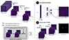 |
Fig. 1. Architecture of the two NNs used in this paper: the convolutional ResNet (A-branch) presented in Sect. 4.1 and the autoencoder ResNet (B-branch) presented in Sect. 4.2. Both networks are based on a residual deep learning architecture detailed in the legend on the bottom left-hand side. The architecture of both networks is similar in the first half and differs in the second half as indicated by the two different branches. |
4.1. Convolutional residual neural network
In the first part, we use a supervised convolutional NN to return the (x, y) pixel coordinates of the BCG in images. The NN architecture consists of a five-layer convolutional residual NN (ResNet) (He et al. 2015), topped with a dense layer. Each residual block is made of two 2D convolutional (Conv2D) layers, each Conv2D layer is followed by a dropout layer. The first Conv2D+DropOut layer feeds into the second. The output of the first Conv2D+DropOut layer is concatenated with the output from the second one. The output of this concatenation then goes through a pooling layer. The Conv2D layers have a ‘relu’ (Agarap 2018) activation function. The pooling was done using another 2D convolutional layer with stride 2. Although this slightly increases the overall network parameters, using convolutional layers with a stride greater than 1 effectively means learning a pooling kernel, which has been demonstrated to increase the expressibility of CNNs (He et al. 2015; Milletari et al. 2016). The final part of the network is composed of a flattening layer, a dense layer, a dropout layer, and, lastly, a dense layer with two neurons to output the (x, y) BCG coordinates. We used a learning rate of lr = 0.0001, a mean squared error loss function, and the Adam optimiser (Kingma & Ba 2017).
The use of ResNet (He et al. 2015) allows us to better deal with vanishing gradients that prevent the accuracy of deep NNs to improve with complexity. In a traditional NN, one layer feeds directly into the next and so on. In that case, in a N-layer network with the initial input being denoted x, each layer gets as an input fn(x), with 1 ≤n ≤ N, such as the network tries to directly learn the function that will produce the desired output H(x). With residual blocks, we incorporate skipped connections: one layer feeds into another layer, but instead of only considering the output of this second layer, we keep the identity of the first one as well. In that case, one layer gets as an input f(x)+x, and the identity is preserved through the following layers as well. The output of each residual block is a global function of x and the identity x, fn(x)+x. As a result, instead of trying to directly match the output such as F(x) = H(x) in a traditional network, using ResNet, we calculated a global residual function as H(x) = F(x)+x and F(x) = H(x)−x. The use of a ResNet with skipped connections enabled us to better retain information present and learnt in the first layers of the NN, which in a traditional network may end up getting lost due to small weights in a layer. It also enabled us to skip entirely one layer if unnecessary, which, in a traditional network is not feasible as all layers depend on the output of the previous ones. The ResNet takes as inputs images of the cluster in all six ugrizy bandpasses of 512 × 512 pixels and returns the pixel coordinates (x, y) of the BCG as its output.
4.2. Convolutional residual autoencoder
In the next part, in an effort to increase the accuracy of the convolutional ResNet and using as a baseline the architecture described in Sect. 4.1, we developed a residual autoencoder that (instead of outputting (x, y) coordinates) returns a probability map with the same inputs. We created two different types of probability maps and compare the results of both in the following section.
4.2.1. Probability masks
First, the probability maps are simply created by drawing a small circular source with a radius of 10 pixels at the position of the BCG, and convoluting the profile with a Gaussian, with a kernel size of 150 pixels and a standard deviation σ = 4. The parameters of the Gaussian were chosen so it would be big enough to cover most of the centre of the BCG profile, and so that the probability in a radius of 5 pixels would be of about 50%.
Then, for comparison, and in an attempt to get even more accurate outputs, the probability maps were obtained by using Gaussian convoluted segmentation maps. The segmentation maps were obtained from the detection code SourcExtractor (Bertin & Arnouts 1996). In the first method, the NN learns to mainly recognise the central region of the BCG; in the second, it is trained using the whole profile and morphology of the BCG. These segmentation maps are obtained only in the z bandpass, in the reddest bandpass, as it is the one with the highest signal-to-noise ratio (S/N). We thus assume the same segmentation map for all six bandpasses. They flag the pixels associated with the BCG as ones and the rest as zeros. Then, we converted these segmentation maps into probability maps by convolving the segmentation maps with a Gaussian profile, as described in the first method. For clusters in which the BCG could not be detected because of deblending issues, the segmentation map is created by drawing a smaller circular source with a radius of 5 pixels and convoluting the profile with a Gaussian. We chose to still include these clusters in the training to infer if the NN would actually manage to outperform usual detection algorithms that tend to miss these sources.
4.2.2. Autoencoder
We used a convolutional residual autoencoder composed of an encoder that will extract the main features from the input and a decoder that will reconstruct the same dimension input using the features extracted by the encoder. The encoder architecture is the same as the ResNet described in Sect. 4.1. The decoder that follows the encoder differs only by the replacement of pooling layers into transpose layers to up-sample instead of down-sample. The final layer of the autoencoder is a transpose layer that will return six probability maps in all six ugrizy filtrebands. We used one last Conv2D layer to compress this output into a single probability map used to detect the BCG. The loss function used here is a binary cross-entropy loss function. The central coordinates of the BCG are associated with the pixel with the highest probability.
5. Performance of the neural networks
Here, we discuss the performance of both NNs described in Sect. 4. We evaluate the accuracy of the trained NNs on the evaluation data of 5362 galaxy clusters. We define an accurately detected BCG if the coordinates of the predicted BCGs are within 10 pixels of the true coordinates of the BCG as given in the cosmoDC2 cluster catalogue. The accuracy is thus defined as the number of accurately detected BCGs over the total number of BCGs in the evaluation sample. The results are summarised in Table A.1.
5.1. Convolutional residual neural network
The convolutional residual NN presented in Sect. 4.1 returns the (x, y) coordinates of the detected BCG.
5.1.1. Accuracy estimation
The spatial distribution of the true BCGs in the cosmoDC2 cluster catalogue and the BCGs detected by the ResNet are shown on Fig. 2. This spatial distribution results from the pre-processing described in Sect. 3, in which clusters were given a random centre shift, up to a distance of 300 kpc from the true centre defined in the cosmoDC2 cluster catalogue. As explained in Sect. 3, this procedure is done in order not only to increase the sample size, but also to take into account uncertainties on the cluster coordinates and redshifts, as could be expected from catalogues obtained from real observations. This also insures that the NNs does not just detect the brightest peak the closest to the image centre as the BCG. As indicated by the very similar spatial distributions on Fig. 2, the NN is able to detect BCGs in a rather large area on the image, and not only in the very centre.
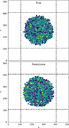 |
Fig. 2. Spatial distribution of the BCGs in the evaluation sample. The true coordinates as per the cosmoDC2 cluster catalogue are shown on the top, whereas the detected coordinates by the NN are shown on the bottom. |
We show in the left panel of Fig. 3 the comparison between the (x, y) coordinates of the BCGs in the evaluation sample as predicted by the convolutional ResNet described in Sect. 4.1 and the true coordinates. We find a good correlation between the predicted and true coordinates, as most points are aligned along the main axis. Both x and y coordinates have a very strong correlation coefficient between the predicted and true coordinates of respectively rx = 0.95 and ry = 0.96. The observed systematics with high (respectively low) values of x and y being underestimated (respectively overestimated) are due to the fact that BCGs in the training sample are located in a radius of 300 kpc in an image of a fixed size of 1.5 comoving Mpc (see Fig. 2). The NN may thus be learning to search for the BCG in this radius, putting upper and lower limits on the pixel interval in which the BCG can be found.
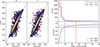 |
Fig. 3. Accuracy of the convolutional ResNet described in Sect. 4.1. Left: (x, y) predicted coordinates of the BCGs as a function of their true (x, y) coordinates as given in the cosmoDC2 simulation. The figure shown here is obtained for the BCGs in the evaluation sample. The colour bar represents the number density of points, with yellow representing higher density. Right: Histogram of the difference between the predicted and true (x, y) coordinates of the BCGs in the evaluation sample as detected by the ResNet (top). The red and blue histograms represent the x and y coordinates respectively. Accuracy of the convolutional ResNet depending on the defined resolution considered for a well-detected BCG (bottom panel). The blue and red lines correspond to an accuracy of 80% and 90%, respectively. |
The distribution of the difference between the (x, y) predicted and true coordinates is shown on the right top panel of Fig. 3. The distribution is a Gaussian with a mean and standard deviation of (μx=−1.51,σx = 16.22) and (μy=−1.53,σy = 15.56) for the x and y coordinates, respectively.
The bottom right panel of Fig. 3 shows the accuracy of the ResNet depending on the resolution defined to consider a BCG as accurately detected. We find that for the defined resolution of 10 pixels, 81% of the BCGs in the evaluation sample have been accurately detected. To obtain an accuracy of at least 90%, we would need to increase the resolution to up to 26 pixels. However, this limit is too big as the BCG halo may extend up to 20 pixels on our images, so at these distances, the predicted position would fall outside of these borders.
5.1.2. Identification of outliers
In Fig. 4, we verify whether the outliers with big differences are associated with the clusters at higher redshift. Indeed, at high-z, galaxies are less resolved, have lower S/N, and we expect photometric measurements to be less precise; in addition, the red sequence is not expected to be as well-defined because the bandpasses are not red enough to constrain the 4000 Å break. All these reasons could cause the NN to not train as efficiently at these distances. However, we find that outliers are found at all redshifts, without any distinction between low-z and high-z clusters.
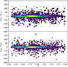 |
Fig. 4. Difference between the (x, y) predicted and true coordinates of the BCGs in the evaluation sample, using the convolutional ResNet, and the clusters’ redshifts. The colour bar represents the number density of points, with yellow representing a higher density. |
A visual inspection of the outliers shows that clusters that present the biggest offsets tend to be mostly clusters with more complex structures where two or more galaxies appear to be comparable to the BCG as defined in the cosmoDC2 catalogue. Indeed, in not so few cases, the defined BCGs in clusters may not be much different from the second or third brightest galaxies, making the distinction with the actual BCG not so straightforward. In such clusters, where several galaxies appear to be equally good BCG candidates, we find that the ResNet returns a BCG position that is located in between of these candidates. Such examples are given on Fig. 5 where the detected BCG (red cross) appears offset from the true BCG (white cross) because of the presence of a comparable galaxy in the field of the cluster. We note that in such complex cases, the detection of the true BCG or the second BCG candidate would both be acceptable as both galaxies appear to be very similar in sizes, luminosities, and location in the cluster relative to the galaxy density distribution. However, as can be seen on Fig. 5, the network returns an in-between position that does not correspond to any object. Although this NN appears to be relatively efficient, with an accuracy of 81%, it does not allow us to automatically identify bad detections.
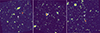 |
Fig. 5. Example of three clusters in the LSST-DP0.2 simulation where the predicted BCG, indicated by the white cross, is offset from the true BCG from the cosmoDC2 catalogue, indicated by the red cross. |
5.2. Convolutional residual autoencoder
We identified the BCG position as detected by the convolutional ResNet autoencoder described in Sect. 4.2 as the pixel on the output probability map with the highest probability.
5.2.1. Accuracy estimation
We first discuss the results obtained by training the NNs using probability maps with the BCG as a circular gaussian convoluted source. We then compare these results with those obtained by using the Gaussian convoluted segmentation maps.
Similarly to the results found in the previous Sect. 5.1 (see Fig. 2, Fig. 3, and Fig. 4), the coordinates of the detected BCGs are very well correlated with those of their true BCGs (see left panel of Fig. 6) with correlation coefficients of r = 0.96 for both (x, y) coordinates. There is also no bias with redshift.
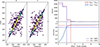 |
Fig. 6. Accuracy of the convolutional ResNet autoencoder described in Sect. 4.2. Left: (x, y) predicted coordinates of the BCGs as a function of their true (x, y) coordinates as given in the cosmoDC2 simulation. The figure shown here is obtained for the BCGs in the evaluation sample. The colour bar represents the number density of points, with yellow representing higher density. Right: Histogram of the difference between the predicted and true (x, y) coordinates of the BCGs in the evaluation sample as detected by the ResNet autoencoder (top). The red and blue histograms represent the x and y coordinates respectively. Accuracy of the ResNet autoencoder depending on the defined resolution considered for a well-detected BCG (bottom). The blue and red lines correspond to an accuracy of 80% and 90%, respectively. |
The accuracy of the autoencoder compared to the simple ResNet is significantly better by a magnitude. Indeed, we find that the accuracy of the autoencoder increases the accuracy to 95%, also with much better resolution. As can be seen in the right panel of Fig. 6, 93% of detected BCGs have an offset of less than 3 pixels. This can be explained by the difference in outputs between the convolutional ResNet and the residual autoencoder. On one hand, the simple ResNet compresses all the information contained in the input and outputs a single set of coordinates (x, y). The autoencoder on the other hand restores the information extracted from the input back to its original format. In the case of confusion between several BCG candidates, as could be seen in Fig. 5, the autoencoder can flag each of these detections with different weights. Such output probabily maps are shown on Fig. 7. The clusters shown are the same as the ones shown on Fig. 5. The true position of the BCG in the cosmoDC2 catalogue is indicated by a red cross, the position of the detected BCG by the ResNet autoencoder associated with the pixel with the highest probability is indicated by a blue cross, and for comparison, the position of the (x, y) coordinates of the detected BCG by the ResNet detailed in Sect. 4.1 is indicated by a white cross. In all of these three examples, in which the ResNet described in Sect. 4.1 failed to accurately detect the BCG and pointed to the background, the autoencoder ResNet manages to correctly detect them with a probability of more than 90%. It can be noted that a second source is flagged as a potential BCG on these three examples, although with much lower probability (around 60% for first two examples, less than 20% for the third example). The coordinates returned by the ResNet in Sect. 4.1 appears to fall in-between the true BCG position and the second flagged source. We confirm in this way that the ResNet in Sect. 4.1 appears to have been confused by the presence of several BCG candidates, and the output format did not allow it to properly convey this information.
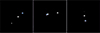 |
Fig. 7. Example of the same three clusters as shown in Fig. 5. The probability maps were obtained using the ResNet autoencoder described in Sect. 4.2. The blue cross correspond to the position of the detected BCG, associated with the pixel with the highest probability. For comparison are also overlaid the red and white crosses in Fig. 5 corresponding to the position of the predicted BCG by the convolutional ResNet described in Sect. 4.1 and the true BCG respectively. |
We show in Fig. 8 the distribution of the probabilities of the detected BCGs in our evaluation sample and the probabilities as a function of the offset between the detected and true coordinates of the BCGs. In total, out of the 5362 clusters in the evaluation sample, 5281 (98%) of them have a detected BCG with a probability higher than 70%. However, as illustrated on the right panel of Fig. 8, not all of these BCGs are accurate. Indeed, we find that only 5032 (94%) BCGs out of 5362 have both a high probability and an accurate detected BCG. The difference of 249 galaxies comes mainly from the above mentioned clusters with several BCG candidates. The NN thus estimated that one of the other candidates was more likely to be the BCG. We note that we do not necessarily consider those as bad detections, as they are very comparable to the BCG defined in the cosmoDC2 catalogue. We also find that about 1% of our evaluation sample has a well-predicted BCG but a low detection probability of less than 70%. A small cloud of points can be found with probabilities close to zero. We discuss the nature of these objects in Sect. 5.2.2.
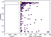 |
Fig. 8. Left: Histogram of the BCG probabilities for the detected BCGs in the evaluation sample. Right: Detection probabilities of the detected BCGs as a function of the offset between the predicted and true coordinates of the BCG. The colour bar represents the number density of points, with yellow representing higher density. |
We now discuss the performance of the NN using more complex segmentation-based probability maps in the training, as opposed to simple circular Gaussian sources. The use of segmentation maps to generate probability maps allows us to retain information on the morphology of the BCG, contrary to the circular sources which just indicate the centre of the BCG. We could assume the use of more complex outputs in the training would result in better performance, as additional information is contained in them. However, unexpectedly, we find that the use of more complex probability maps during the training, based on segmentation maps, does not improve the accuracy of the NN. The autoencoder performs just as well with both sets of outputs. This may indicate that, on the galactic scale, the morphology of the BCG does not play a significant role in the training, and that the NN puts more weight on the central luminosity of the galaxy to identify the BCG.
5.2.2. Identification of outliers
We investigate the nature of the BCGs detected by the autoencoder with an almost null probability, as can be seen on Fig. 8. Those correspond to clusters for which the NN could not detect any BCGs. A visual inspection of these clusters reveals that those belong to two main categories: first, BCGs close to another object causing deblending issues; second, red BCGs which have a very low S/N, even on the reddest filtre, which complicates their detection.
6. Discussion
6.1. Comparison with red sequence based algorithms
With the aim of justifying the use of deep learning for BCG detection, we sought to compare the efficiency of the NNs described in this section to more traditional methods that rely solely on photometry. In this work, we compared the results obtained with those of Chu et al. (2021) which is based on a red sequence extraction method. The definition of a BCG in this paper is similar to the one used in Chu et al. (2021); namely, the BCG is defined as the brightest cluster galaxy that lies close to the cluster centre. In a first approach, we only considered a sub-sample of mid-redshift clusters, from redshifts 0.4 ≤z≤ 0.7. The upper limit at z ≤ 0.7 is the usual detection limit of most red sequence-based algorithms, as at higher redshifts, most surveys do not go far enough in the infrared to constrain the 4000 Å break to obtain sufficiently good photo-z estimations. This study was carried out based on a sub-sample of 677 clusters between 0.4 ≤ z ≤ 0.7.
Chu et al. (2021) detected the BCG in a sample of 132 clusters observed with the Hubble Space Telescope, from a redshift of z = 0.1 to z = 1.8. The method described in that paper was adapted to fit the given data, enabling Chu et al. (2021) to accurately detect all red BCGs in their samples. We would expect the performance of this method to be less efficient for another given set of data and further tweaking of the parameters would be necessary. Also, the main difference between the sample used in Chu et al. (2021) and this work is the fact that the present paper uses simulation data. In the description paper of the LSST simulated sky survey (LSST Dark Energy Science Collaboration 2022), the colours of the simulated LSST galaxies are compared with observed colours of galaxies in the SDSS. They show that the colour distributions of the simulated LSST galaxies are not a perfect match to the distributions of SDSS galaxies, but similar enough to be used for science purposes such as studies of the luminosity or stellar mass function of galaxies, but may not be accurate enough for precise photometric redshift measurements. These differences lead us not to use exactly the same limits as in Chu et al. (2021). Based on the same guideline as Chu et al. (2021), we here adapt and try to optimise the method for our LSST-DP0.2 simulated data for a fair comparison.
We summarise the method presented in Chu et al. (2021) hereafter. First, foreground sources are identified and excluded using their photometric luminosities. Then, the red sequence is extracted using aperture photometry done with the source detection code SourcExtractor. The measured colours of the galaxies in the field are compared to a model, and galaxies with a similar colour to the model are considered as being part of the cluster’s red sequence. Using this red sequence, they calculate the galaxy density around a given candidate to determine if that galaxy is isolated or in the central region of the galaxy distribution of the cluster. The BCG is detected as the brightest galaxy in a galaxy overdensity in the image.
We note that since the cosmoDC2 already provides photometric measurements of the magnitudes and sizes of the galaxies in the simulation, instead of SourcExtractor measured properties, we use the cosmoDC2 measurements in the retrieved catalogues. Magnitudes are taken as the parameters mag_{ugrizy}_lsst in the catalogues, and ellipticities as the ellipticity_true parameter.
In the following, we provide a detailed summary of the method used in Chu et al. (2021) and the present work. We first select all galaxies in the cosmoDC2 simulation in a 1.5 Mpc aperture in the field of the cluster with a magnitude mag_r_lsst < 28, the limiting magnitude of the survey. We then filtre out foreground galaxies by computing their ‘pseudo-absolute magnitude’, which is the absolute magnitude of a given object computed at the cluster’s redshift, considering their measured luminosities on the image. Foreground galaxies, via this parameter, would then appear too bright. We thus exclude all objects with pseudo absolute magnitudes brighter than –26 mag in both the i and z bands. Edge-on galaxies are identified if they have ellipticities ellipticity_true ≤ 2.6.
The red sequence is then extracted by selecting all galaxies with a colour i − z that is less than 0.6 mag farther than a model. The model is based on a spectral energy distribution from Bruzual & Charlot (2003), which assumes a star formation history that decreases exponentially from a single burst at zf = 5 with τ = 0.5 Gyr, solar metallicity and Chabrier initial mass function. Sorting through luminosities, we then calculate the galaxy density around every BCG candidate to look for red galaxies overdensities.
Doing this, we find that the red sequence algorithm that is used for most wide astronomical surveys, applied to our LSST-DP0.2 simulation, has a 70% accuracy. The 30% of bad detections, similar to the two other methods, also come from the presence of multiple BCG candidates. Because of photometric uncertainties, some galaxies, if close in luminosity to the true BCG, may have a slightly brighter measured magnitude which explains its detection instead of the true BCG. Most of the errors, however, come from the bad extraction of the red sequence galaxies with the presence still of interlopers in the red sequence catalogue. These interlopers may remain because of photometric uncertainties (particularly for sources which need to be deblended) or because they may appear to have similar colours to the cluster’s galaxies although being foreground sources. This method also requires more pre-processing with the generation of photometric catalogues and the following red sequence extraction. In this way, we were able to significantly improve the performance of our detection method by more than 20% by implementing deep learning.
In summary, our autoencoder is thus superior to red sequence BCG-finders in several aspects. First, it is both faster and requires less memory as it does not require the generation of photometric catalogues. Second, it detects the BCG with a very good resolution of less than 5 pixels. And finally, it returns a confidence level for each detection which enables to filtre out bad detections, which can be difficult to compute with photometric methods.
6.2. Definition of the BCG
In this study, the BCG is defined as the brightest galaxy in the central region of the cluster, as defined in the cosmoDC2 catalogue. However, some authors would argue that the BCG should be the brightest galaxy of the cluster, independently of its distance from the centre of the cluster. This definition of what a BCG should be can cause inconsistencies as different definitions may lead to the identification of different BCGs. A massive galaxy may be displaced from the centre of its host cluster due to recent merging events (Patel et al. 2006; Hashimoto et al. 2014; De Propris et al. 2020; Chu et al. 2021). As a result, in order to detect these off-centred BCGs using the presented NNs, they will need to be retrained using the new BCG coordinates.
6.3. Presence of multiple BCGs
As mentioned previously, some clusters may present not only one but two or more BCGs that differ only very slightly in brightness and size. In occurrence, a supercluster may present one BCG in each of its sub-structure. For merging clusters, with their BCGs bound to merge together at some point, it is also complicated to determine which is the true BCG. It is still unclear if a slightly brighter but offset massive galaxy would be a better candidate than a slightly less bright but more central galaxy as a BCG. The galaxy detected by the autoencoder, which may not coincide with the BCG in the cosmoDC2 catalogue, may be just as good of a BCG candidate. For these reasons, and considering these uncertainties, we could consider that some of the bad detections made by the autoencoder presented in Sect. 4.2 may actually be reasonable. We are therefore likely underestimating the autoencoder’s accuracy.
The ability of the autoencoder to detect several candidates is also a very strong feature of the network. This feature may be very useful for ICL studies for example, in which the question of whether to consider only one or two BCGs to measure the ICL fraction in clusters is still pending. The autoencoder will allow us not only to identify these clusters with several BCGs, but also to give the positions of these different candidates with relative weights. A simple way to identify these clusters automatically would be to apply a source detection code on the output probability maps and select those with more than one detected sources. It is to be noted however, that the autoencoder described in this paper was not trained with probability maps that contain multiple sources. It may thus be refined by implementing these additional sources in the probability maps used in the training, attributing to these secondary sources a probability that is a function of the ratio of size, luminosity, and distance from the true BCG.
6.4. Simulation to observations
It is important to note, once again, that the NNs described in this paper were trained using simulation data and not real observational data. Observational data differs from simulated data by the presence of noise and artefacts that can not be perfectly reproduced with simulations. Also, the LSST DP0.2 simulation does not include AGNs, strong lenses, solar system objects, or more importantly low surface brightness diffuse features such as tidal streams or ICL which is a very strong feature associated with the stellar halo of the BCG. As a result, the current trained network can not be applied directly to the future LSST data release. Indeed, studies such as Belfiore et al. (2025) for example have shown the gap between real and simulated nebulae and the effect of the nature of the sample on the training of the NN. The current trained models could be applied on real images by continuing the training using real LSST images, using as training a catalogue of clusters confirmed spectroscopically with identified BCGs. This form of transfer learning from simulation to real observational data would be a better approach than training a new model from scratch using only the future data release images. We can expect the current network to have learned the main features for BCG detection, and so the trained neural weights to be approximately correct. We may hope for the NNs to learn additional features from the presence of ICL or tidal streams to better detect the BCGs on the real images, and adjust these weights, as those are features which are mostly associated with BCGs. In such a case, we could expect the use of segmentation maps in the training to actually increase the performance of the autoencoder, whereas in this paper, they are not essential.
In the meantime, the performance of the autoencoder applied on the real future data release from LSST may be estimated using data from the HSC-SSP survey. HSC-SSP is very comparable to the future LSST survey in terms of depth, resolution and other imaging properties, but differs mainly by its much smaller footprint and the lack of the u-band. The network may be trained again using transfer learning by using images from HSC-SSP to estimate its robustness on real data. This will be addressed in a follow-up paper.
7. Conclusion
In this work, we made use of machine learning in the form of deep NNs to detect BCGs on optical images in preparation for the upcoming LSST data release. With that aim, we used simulation images from the LSST Data Preview DP0.2, which provides images in all six ugrizy filtre bands, obtained following the simulated LSST cadence up to the five-year mark. We used two different NNs: the first one (described in Sect. 4.1) is a convolutional ResNet that takes as input images in all six bandpasses and outputs the (x, y) pixel coordinates of the BCG on the images. This very straightforward method returns 80% of good detections in our evaluation sample. However, we find that this method might not be reliable in cases where the cluster presents multiple BCG candidates with similar properties. In such cases, the ResNet will return a position that is between the positions of these candidates. The simple binary output format is thus not suited for this study. The lack of a flag to differentiate the good from the bad detections prevented us from constructing a pure and complete BCG catalogue without post-processing. A simple post-processing procedure to check whether the coordinates returned by the ResNet are correct could consist of checking, for example, that these coordinates are indeed associated with a bright galaxy in the central region of the image using a source detection code.
In an effort to bypass this obstacle, we made use of an autoencoder ResNet, which is described in Sect. 4.2. Contrary to the traditional ResNet which outputs coordinates, the autoencoder outputs a probability map of the same format as the input images. The pixel with the maximum probability is associated with the position of the BCG. The autoencoder has two main advantages compared to the traditional ResNet: it provides a confidence level (represented as probabilities) to identify which detections may be faulty and it indicates the position of all potential candidates with relative weights. The autoencoder increases the performance of the ResNet from 80% to 95%.
The main challenge for our NNs is to differentiate between the different possible candidates in the field. In comparison, algorithms that rely on photometry must deal with a prior problem, namely, removing interlopers such as the foreground and background sources to extract the red sequence accurately. The presence of a nearby cluster, on top of photometric uncertainties, makes the extraction of the red sequence all the more difficult and these algorithms unreliable for big surveys. The NNs appear to be dealing with these problems better than the red sequence finder algorithms.
One common point of contention for all three methods is the deblending of close sources. BCGs hidden in the halo of a foreground source are likely not to be detected by either method. This issue is unfortunately very common in detection problems and is challenging even for NNs. Efforts to solve this ongoing problem have been made. In particular, Burke et al. (2019) developed new deep learning techniques that have allowed them to cleanly deblend 98% of galaxies in a crowded field. Their method could be associated with ours in order to boost the performance of our method and potentially retrieve those blended BCGs in our final catalogue. Moreover, the fact that undetected BCGs primarily suffer from deblending issues or low S/Ns suggests that incompleteness is correlated with luminosity, local galaxy density, and redshift. The confidence levels produced as output by our autoencoder (see Fig. 6) provide a natural diagnostic: we can measure detection efficiency by binning BCGs in this multi-dimensional parameter space and track the probability distribution. This selection function could then be used to correct incompleteness by incorporating it into subsequent studies of BCG luminosity or mass functions.
We can compare the NNs presented in this paper to one presented by Janulewicz et al. (2025). They used machine learning to detect BCGs in large surveys such as the SDSS, using mock observations from The Three Hundred project and real SDSS images for the training. Their network appears to have very good robustness up to z = 0.6 once applied to real data. In comparison, our method seems to be robust up to z = 2.0 but has not yet been tested on observational data.
The use of simulated data to train our NNs instead of real observational data also needs to be addressed, especially as the final goal is to apply these NNs to the future Rubin-LSST data releases. As discussed in Sect. 6, the nature of the training sample is an important parameter that should not be overlooked, as studies such as Belfiore et al. (2025) have shown its impact on the accuracy of a model. This problem will be addressed in a follow-up paper which will make use of HSC-SSP data to estimate the expected accuracy of the NNs presented in this paper to real observations.
We show that NNs can be a great tool for BCG detection. Although they are often seen as a black box lacking physical motivations, the two NNs presented here perform better than the basic red sequence extractor by a magnitude. The implementation of probability maps also allows us to flag inconclusive detections. The resulting BCG catalogue, constructed with the help of NNs, will ultimately produce an inventory of all BCGs in clusters in the southern hemisphere surveyed by LSST over the course of the next ten years, which can then be used for various studies. The combination of studies of the structural physical properties of BCGs, along with with studies of the ICL and tidal streams associated with the BCGs from local to proto-clusters (z > 2), will improve our understanding of galaxy formation and evolution in dense environments. The NNs presented in this paper will enable us to obtain a pure BCG catalogue from the LSST data release in a fast and efficient way.
Acknowledgments
We thank the referee for relevant comments and suggestions to this work and paper. We also thank Florence Durret for her insight in the redaction of this paper. This research utilised the Sunrise HPC facility supported by the Technical Division at the Department of Physics, Stockholm University. This paper makes use of LSST Science Pipelines software developed by the Vera C. Rubin Observatory. We thank the Rubin Observatory for making their code available as free software at https://pipelines.lsst.io. This work has been enabled by support from the research project grant ‘Understanding the Dynamic Universe’ funded by the Knut and Alice Wallenberg Foundation under Dnr KAW 2018.0067. LD acknowledges travel support from Elisabeth och Herman Rhodins Minne and from the Swedish-French Foundation. JJ acknowledges the hospitality of the Aspen Center for Physics, which is supported by National Science Foundation grant PHY-1607611. The participation of JJ at the Aspen Center for Physics was supported by the Simons Foundation. JJ and LD acknowledge support by the Swedish Research Council (VR) under the project 2020-05143 – “Deciphering the Dynamics of Cosmic Structure”. JJ and LD further acknowledge support by the Simons Collaboration on “Learning the Universe”. This work has been done within the Aquila Consortium (https://www.aquila-consortium.org).
References
- Abadi, M., Agarwal, A., Barham, P., et al. 2015, TensorFlow: Large-Scale Machine Learning on Heterogeneous Systems, software available from tensorflow.org [Google Scholar]
- Agarap, A. F. 2018, arXiv e-prints [arXiv:1803.08375] [Google Scholar]
- Ascaso, B., Aguerri, J. A. L., Varela, J., et al. 2010, ApJ, 726, 69 [Google Scholar]
- Bai, L., Yee, H., Yan, R., et al. 2014, ApJ, 789, 134 [Google Scholar]
- Baron, D. 2019, Machine Learning in Astronomy: a practical overview [Google Scholar]
- Baum, W. A. 1959, PASP, 71, 106 [Google Scholar]
- Belfiore, F., Ginolfi, M., Blanc, G., et al. 2025, Machine learning the gap between real and simulated nebulae: A domain-adaptation approach to classify ionised nebulae in nearby galaxies [Google Scholar]
- Bernardi, M. 2009, MNRAS, 395, 1491 [Google Scholar]
- Bertin, E., & Arnouts, S. 1996, A&AS, 117, 393 [NASA ADS] [CrossRef] [EDP Sciences] [Google Scholar]
- Biermann, P., & Tinsley, B. M. 1975, A&A, 41, 441 [NASA ADS] [Google Scholar]
- Bosch, J., Armstrong, R., Bickerton, S., et al. 2018, PASJ, 70, S5 [Google Scholar]
- Bosch, J., AlSayyad, Y., Armstrong, R., et al. 2019, ASP Conf. Ser., 523, 521 [Google Scholar]
- Bruzual, G., & Charlot, S. 2003, MNRAS, 344, 1000 [NASA ADS] [CrossRef] [Google Scholar]
- Burke, C. J., Aleo, P. D., Chen, Y.-C., et al. 2019, MNRAS, 490, 3952 [NASA ADS] [CrossRef] [Google Scholar]
- Canepa, L., Brough, S., Lanusse, F., Montes, M., & Hatch, N. 2025, Measuring the intracluster light fraction with machine learning [Google Scholar]
- Cho, J., Lee, K., Shin, E., Choy, G., & Do, S. 2015, arXiv e-prints [arXiv:1511.06348] [Google Scholar]
- Chu, A., Durret, F., & Márquez, I. 2021, A&A, 649, A42 [NASA ADS] [CrossRef] [EDP Sciences] [Google Scholar]
- Chu, A., Sarron, F., Durret, F., & Márquez, I. 2022, A&A, 666, A54 [NASA ADS] [CrossRef] [EDP Sciences] [Google Scholar]
- De Lucia, G., Springel, V., White, S. D. M., Croton, D., & Kauffmann, G. 2006, MNRAS, 366, 499 [NASA ADS] [CrossRef] [Google Scholar]
- De Propris, R., West, M. J., Andrade-Santos, F., et al. 2020, MNRAS, 500, 310 [Google Scholar]
- de Vaucouleurs, G. 1961, ApJS, 5, 233 [NASA ADS] [CrossRef] [Google Scholar]
- DeMaio, T., Gonzalez, A. H., Zabludoff, A., et al. 2020, MNRAS, 491, 3751 [Google Scholar]
- Dressler, A. 1980, ApJ, 236, 351 [Google Scholar]
- Dressler, A. 1984, ARA&A, 22, 185 [NASA ADS] [CrossRef] [Google Scholar]
- Dubois-Felsmann, G., Economou, F., Lim, K.-T., et al. 2019, https://ldm-542.lsst.io [Google Scholar]
- Durret, F., Tarricq, Y., Márquez, I., Ashkar, H., & Adami, C. 2019, A&A, 622, A78 [NASA ADS] [CrossRef] [EDP Sciences] [Google Scholar]
- Edwards, L. O. V., Salinas, M., Stanley, S., et al. 2019, MNRAS, 491, 2617 [Google Scholar]
- Golden-Marx, J. B., Miller, C. J., Zhang, Y., et al. 2022, ApJ, 928, 28 [NASA ADS] [CrossRef] [Google Scholar]
- Hashimoto, Y., Henry, J. P., & Boehringer, H. 2014, MNRAS, 440, 588 [Google Scholar]
- He, K., Zhang, X., Ren, S., & Sun, J. 2015, Deep Residual Learning for Image Recognition [Google Scholar]
- Heitmann, K., Finkel, H., Pope, A., et al. 2019, ApJS, 245, 16 [NASA ADS] [CrossRef] [Google Scholar]
- Hickson, P., Richstone, D. O., & Turner, E. L. 1977, ApJ, 213, 323 [Google Scholar]
- Hubble, E. P. 1936, Realm of the Nebulae [Google Scholar]
- Huertas-Company, M., & Lanusse, F. 2023, PASA, 40, e001 [NASA ADS] [CrossRef] [Google Scholar]
- Ivezić, Ž., Kahn, S. M., Tyson, J. A., et al. 2019, ApJ, 873, 111 [Google Scholar]
- Janulewicz, P., Webb, T. M. A., & Perreault-Levasseur, L. 2025, ApJ, 981, 117 [Google Scholar]
- Jenness, T., Bosch, J. F., Salnikov, A., et al. 2022, SPIE Conf. Ser., 12189, 1218911 [Google Scholar]
- Jurić, M., Ciardi, D. R., Dubois-Felsmann, G. P., & Guy, L. P. 2019, https://lse-319.lsst.io [Google Scholar]
- Kingma, D. P., & Ba, J. 2017, Adam: A Method for Stochastic Optimization [Google Scholar]
- Korytov, D., Hearin, A., Kovacs, E., et al. 2019, ApJS, 245, 26 [NASA ADS] [CrossRef] [Google Scholar]
- Larson, R. B. 1975, MNRAS, 173, 671 [NASA ADS] [CrossRef] [Google Scholar]
- Lauer, T. R., Postman, M., Strauss, M. A., Graves, G. J., & Chisari, N. E. 2014, ApJ, 797, 82 [Google Scholar]
- Lietzen, H., Tempel, E., Heinämäki, P., et al. 2012, A&A, 545, A104 [NASA ADS] [CrossRef] [EDP Sciences] [Google Scholar]
- LSST Dark Energy Science Collaboration (Abolfathi, B., et al.) 2022, DESC DC2 Data Release Note [Google Scholar]
- Marchant, A. B., & Shapiro, S. L. 1977, ApJ, 215, 1 [Google Scholar]
- Marini, I., Borgani, S., Saro, A., et al. 2022, MNRAS, 514, 3082 [NASA ADS] [CrossRef] [Google Scholar]
- Milletari, F., Navab, N., & Ahmadi, S.-A. 2016, V-Net: Fully Convolutional Neural Networks for Volumetric Medical Image Segmentation [Google Scholar]
- Moriwaki, K., Nishimichi, T., & Yoshida, N. 2023, Rep. Prog. Phys., 86, 076901 [NASA ADS] [CrossRef] [Google Scholar]
- Nelson, A. E., Simard, L., Zaritsky, D., Dalcanton, J. J., & Gonzalez, A. H. 2002, ApJ, 567, 144 [NASA ADS] [CrossRef] [Google Scholar]
- Ntampaka, M., Avestruz, C., Boada, S., et al. 2021, The Role of Machine Learning in the Next Decade of Cosmology [Google Scholar]
- Oemler, A. J. 1974, ApJ, 194, 1 [NASA ADS] [CrossRef] [Google Scholar]
- O’Mullane, W., Economou, F., Huang, F., et al. 2024, ASP Conf. Ser., 535, 227 [Google Scholar]
- Partridge, R. B., & Peebles, P. J. E. 1967, ApJ, 147, 868 [Google Scholar]
- Patel, P., Maddox, S., Pearce, F. R., Aragon-Salamanca, A., & Conway, E. 2006, MNRAS, 370, 851 [Google Scholar]
- Pearson, W. J., Santos, D. J. D., Goto, T., et al. 2024, A&A, 686, A94 [NASA ADS] [CrossRef] [EDP Sciences] [Google Scholar]
- Postman, M., & Geller, M. J. 1984, ApJ, 281, 95 [Google Scholar]
- Querejeta, M., Eliche-Moral, M. C., Tapia, T., et al. 2015, A&A, 579, L2 [NASA ADS] [CrossRef] [EDP Sciences] [Google Scholar]
- Rood, H. J., Page, T. L., Kintner, E. C., & King, I. R. 1972, ApJ, 175, 627 [Google Scholar]
- Roos, N., & Norman, C. A. 1979, A&A, 76, 75 [NASA ADS] [Google Scholar]
- Rykoff, E. S., Rozo, E., Busha, M. T., et al. 2014, ApJ, 785, 104 [Google Scholar]
- Sawala, T., Frenk, C., Jasche, J., Johansson, P. H., & Lavaux, G. 2023, Distinct distributions of elliptical and disk galaxies across the Local Supercluster as a ΛCDM prediction [Google Scholar]
- Sohn, J., Geller, M. J., Diaferio, A., & Rines, K. J. 2020, ApJ, 891, 129 [NASA ADS] [CrossRef] [Google Scholar]
- Sohn, J., Geller, M. J., Vogelsberger, M., & Damjanov, I. 2022, ApJ, 931, 31 [NASA ADS] [CrossRef] [Google Scholar]
- Spitzer, L. J., & Baade, W. 1951, ApJ, 113, 413 [NASA ADS] [CrossRef] [Google Scholar]
- Stopyra, S., Peiris, H. V., Pontzen, A., Jasche, J., & Natarajan, P. 2021, MNRAS, 507, 5425 [Google Scholar]
- Stott, J. P., Collins, C. A., Burke, C., Hamilton-Morris, V., & Smith, G. P. 2011, MNRAS, 414, 445 [Google Scholar]
- Sureshkumar, U., Durkalec, A., Pollo, A., et al. 2024, A&A, 686, A40 [NASA ADS] [CrossRef] [EDP Sciences] [Google Scholar]
- Takeda, Y., Kashikawa, N., Ito, K., et al. 2024, ApJ, 977, 81 [Google Scholar]
- The LSST Dark Energy Science Collaboration (Abolfathi, B., et al.) 2021, ApJS, 253, 31 [CrossRef] [Google Scholar]
- Toomre, A. 1977, in Evolution of Galaxies and Stellar Populations, eds. B. M. Tinsley, D. C. Larson, & R. B. Gehret, 401 [Google Scholar]
- West, M. J., de Propris, R., Bremer, M. N., & Phillipps, S. 2017, Nat. Astron., 1, 0157 [Google Scholar]
- Yang, L., Silverman, J., Oguri, M., et al. 2024, MNRAS, 531, 4006 [Google Scholar]
Appendix A: Performance of the detection methods
Comparison of the performances of the detection methods.
All Tables
All Figures
|
Fig. 1. Architecture of the two NNs used in this paper: the convolutional ResNet (A-branch) presented in Sect. 4.1 and the autoencoder ResNet (B-branch) presented in Sect. 4.2. Both networks are based on a residual deep learning architecture detailed in the legend on the bottom left-hand side. The architecture of both networks is similar in the first half and differs in the second half as indicated by the two different branches. |
| In the text | |
|
Fig. 2. Spatial distribution of the BCGs in the evaluation sample. The true coordinates as per the cosmoDC2 cluster catalogue are shown on the top, whereas the detected coordinates by the NN are shown on the bottom. |
| In the text | |
|
Fig. 3. Accuracy of the convolutional ResNet described in Sect. 4.1. Left: (x, y) predicted coordinates of the BCGs as a function of their true (x, y) coordinates as given in the cosmoDC2 simulation. The figure shown here is obtained for the BCGs in the evaluation sample. The colour bar represents the number density of points, with yellow representing higher density. Right: Histogram of the difference between the predicted and true (x, y) coordinates of the BCGs in the evaluation sample as detected by the ResNet (top). The red and blue histograms represent the x and y coordinates respectively. Accuracy of the convolutional ResNet depending on the defined resolution considered for a well-detected BCG (bottom panel). The blue and red lines correspond to an accuracy of 80% and 90%, respectively. |
| In the text | |
|
Fig. 4. Difference between the (x, y) predicted and true coordinates of the BCGs in the evaluation sample, using the convolutional ResNet, and the clusters’ redshifts. The colour bar represents the number density of points, with yellow representing a higher density. |
| In the text | |
|
Fig. 5. Example of three clusters in the LSST-DP0.2 simulation where the predicted BCG, indicated by the white cross, is offset from the true BCG from the cosmoDC2 catalogue, indicated by the red cross. |
| In the text | |
|
Fig. 6. Accuracy of the convolutional ResNet autoencoder described in Sect. 4.2. Left: (x, y) predicted coordinates of the BCGs as a function of their true (x, y) coordinates as given in the cosmoDC2 simulation. The figure shown here is obtained for the BCGs in the evaluation sample. The colour bar represents the number density of points, with yellow representing higher density. Right: Histogram of the difference between the predicted and true (x, y) coordinates of the BCGs in the evaluation sample as detected by the ResNet autoencoder (top). The red and blue histograms represent the x and y coordinates respectively. Accuracy of the ResNet autoencoder depending on the defined resolution considered for a well-detected BCG (bottom). The blue and red lines correspond to an accuracy of 80% and 90%, respectively. |
| In the text | |
|
Fig. 7. Example of the same three clusters as shown in Fig. 5. The probability maps were obtained using the ResNet autoencoder described in Sect. 4.2. The blue cross correspond to the position of the detected BCG, associated with the pixel with the highest probability. For comparison are also overlaid the red and white crosses in Fig. 5 corresponding to the position of the predicted BCG by the convolutional ResNet described in Sect. 4.1 and the true BCG respectively. |
| In the text | |
|
Fig. 8. Left: Histogram of the BCG probabilities for the detected BCGs in the evaluation sample. Right: Detection probabilities of the detected BCGs as a function of the offset between the predicted and true coordinates of the BCG. The colour bar represents the number density of points, with yellow representing higher density. |
| In the text | |
Current usage metrics show cumulative count of Article Views (full-text article views including HTML views, PDF and ePub downloads, according to the available data) and Abstracts Views on Vision4Press platform.
Data correspond to usage on the plateform after 2015. The current usage metrics is available 48-96 hours after online publication and is updated daily on week days.
Initial download of the metrics may take a while.